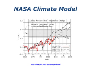
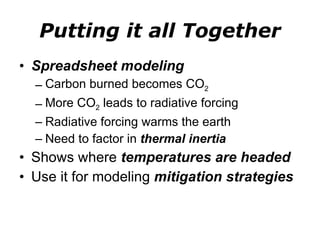
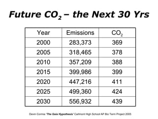
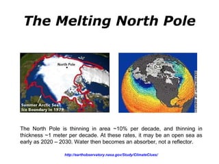
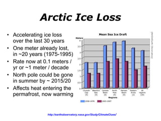
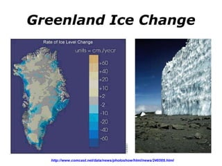
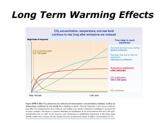
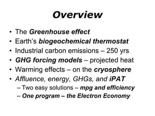
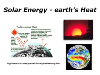
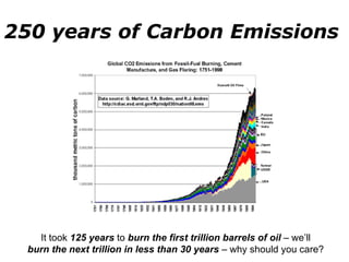
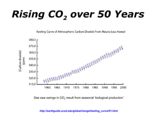
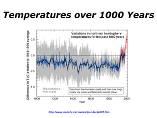
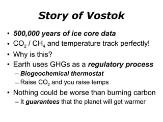
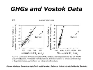
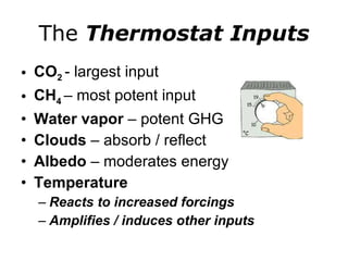
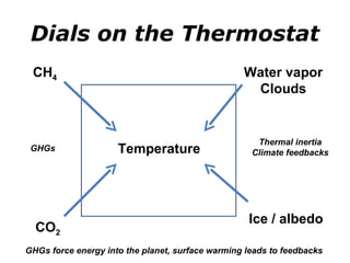
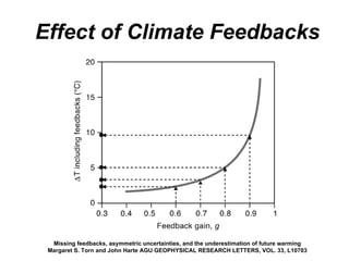
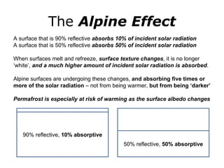
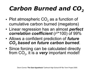
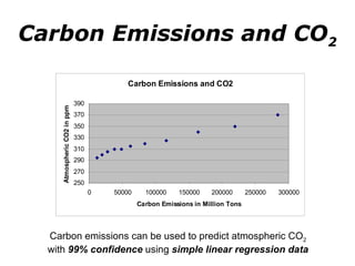
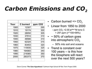
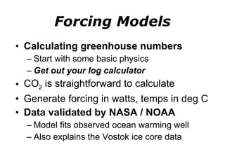
The document discusses the relationship between greenhouse gas emissions, climate change, and global warming based on scientific data and models. It summarizes that carbon emissions can reliably predict increases in atmospheric CO2 levels, which can then be used to model radiative forcing and projected temperature increases. Feedback loops may accelerate warming beyond current predictions. The Arctic and Greenland are already experiencing significant impacts like sea ice loss and melting.

1. Climate Change By the Numbers Robert D. Cormia Foothill College

2. Overview The Greenhouse effect Earth’s biogeochemical thermostat Industrial carbon emissions – 250 yrs GHG forcing models – projected heat Warming effects – on the cryosphere Affluence, energy, GHGs, and iPAT Two easy solutions – mpg and efficiency One program – the Electron Economy

3. Solar Energy - earth’s Heat http://www.ncdc.noaa.gov/oa/climate/globalwarming.html

4. 250 years of Carbon Emissions It took 125 years to burn the first trillion barrels of oil – we’ll burn the next trillion in less than 30 years – why should you care?

5. Rising CO 2 over 50 Years http://earthguide.ucsd.edu/globalchange/keeling_curve/01.html See saw swings in CO 2 result from seasonal ‘biological production’

6. Temperatures over 1000 Years http://www.mala.bc.ca/~earles/ipcc-tar-feb01.htm

7. Story of Vostok 500,000 years of ice core data CO 2 / CH 4 and temperature track perfectly! Why is this? Earth uses GHGs as a regulatory process Biogeochemical thermostat Raise CO 2 and you raise temps Nothing could be worse than burning carbon It guarantees that the planet will get warmer

8. Ice Cores – Story of Vostok

9. Vostok Ice Core Data A perfect correlation between CO 2 , temperature, and sea level For every one ppm CO 2 , sea level rises 1 meter, temp rises .05 C (global) Process takes 100 years to add 1 ppm CO 2 , and reach thermal equilibrium This is not just a correlation, this is a complex and dynamic process , with multiple inputs. Touching one input affects all other inputs , and increases in temperature becomes a further feedback and multiplier of these inputs.

10. Vostok CO 2 and Temperature The relationship between CO 2 and temperature is nearly perfect (r 2 *100 = 99) However, the casual relationship is the basis for significant (expert) controversy Why does this occur?

11. The Vostok Equilibrium Vostok ‘equilibrium’ 100K year cycles earth’s orbital eccentricity Sun heats up the planet Biosphere expands CO 2 maintains temp Otherwise earth would be very cold ~ 0 degrees F CO 2 has not exceeded 280 ppm in the last 500K years and 4 major cycles

12. GHGs and Vostok Data James Kirchner Department of Earth and Planetary Science, University of California, Berkeley

13. The Thermostat Inputs CO 2 - largest input CH 4 – most potent input Water vapor – potent GHG Clouds – absorb / reflect Albedo – moderates energy Temperature Reacts to increased forcings Amplifies / induces other inputs

14. Dials on the Thermostat GHGs force energy into the planet, surface warming leads to feedbacks Thermal inertia Climate feedbacks GHGs CO 2 CH 4 Ice / albedo Water vapor Clouds Temperature

15. Missing feedbacks, asymmetric uncertainties, and the underestimation of future warming Margaret S. Torn and John Harte AGU GEOPHYSICAL RESEARCH LETTERS, VOL. 33, L10703 Effect of Climate Feedbacks

16. The Alpine Effect 90% reflective, 10% absorptive 50% reflective, 50% absorptive A surface that is 90% reflective absorbs 10% of incident solar radiation A surface that is 50% reflective absorbs 50% of incident solar radiation When surfaces melt and refreeze, surface texture changes , it is no longer ‘ white’, and a much higher amount of incident solar radiation is absorbed . Alpine surfaces are undergoing these changes, and absorbing five times or more of the solar radiation – not from being warmer, but from being ‘darker’ Permafrost is especially at risk of warming as the surface albedo changes

17. Carbon Burned and CO 2 Plot atmospheric CO 2 as a function of cumulative carbon burned (megatons) Linear regression has an almost perfect correlation coefficient (r 2 *100) of 99% Allows a confident prediction of future CO 2 based on future carbon burned . Since forcing can be calculated directly from CO 2 , it is a very important model! Devin Cormia ‘The Gaia Hypothesis’ Carlmont High School AP Bio Term Project 2005

18. Carbon Emissions and CO 2 Carbon emissions can be used to predict atmospheric CO 2 with 99% confidence using simple linear regression data

19. Carbon Emissions and CO 2 Carbon burned => CO 2 Linear from 1850 to 2000 - ppm CO 2 =2.55 e 10-4 *M tons C + 297 ppm (r 2 *100=99%) ~ 50% of carbon goes into atmospheric CO 2 50% into soil and oceans Trend is constant over 100 years – is this how the biosphere will react over the next 500 years? Devin Cormia ‘The Gaia Hypothesis’ Carlmont High School AP Bio Term Project 2005

20. Forcing Models Calculating greenhouse numbers Start with some basic physics Get out your log calculator CO 2 is straightforward to calculate Generate forcing in watts, temps in deg C Data validated by NASA / NOAA Model fits observed ocean warming well Also explains the Vostok ice core data

21. Forcing Model from GISS http://www.giss.nasa.gov/ Definitive work in March 2005 1,800 ocean buoys sampling sea temperatures to a depth of ~2,500 meters from 1990 - 2000 Temps must rise 0.66 0 C per 1 W of forcing ‘ Thermal inertia’ of oceans requires 25 to 50 years to experience 60% of total ‘ equilibration’ http://www.giss.nasa.gov/research/news/20050428/ Earth’s Energy Imbalance: Confirmation and Implications James Hansen,* Larissa Nazarenko, Reto Ruedy, Makiko Sato, Josh Willis, Anthony Del Genio, Dorothy Koch, Andrew Lacis, Ken Lo, Surabi Menon, Tica Novakov, Judith Perlwitz, Gary Russell, Gavin A. Schmidt, Nicholas Tausnev – http://www.sciencexpress.org / 28 April 2004 / Page 1/ 10.1126/science.1110252

22. http://www.grida.no/climate/vital/04.htm

23. Earth Out of Balance http://www.giss.nasa.gov/research/news/20050428/

24. Calculating Radiative Forcing 5.35 watts x ln [current ppm CO 2 ] _______________ [historic ppm CO 2 ] Temperature increase C = 2/3 Watts radiative forcing Historic CO 2 is 280 ppm, current CO 2 is 387 ppm

25. NASA Climate Model http://www.giss.nasa.gov/edu/gwdebate/

26. Putting it all Together Spreadsheet modeling Carbon burned becomes CO 2 More CO 2 leads to radiative forcing Radiative forcing warms the earth Need to factor in thermal inertia Shows where temperatures are headed Use it for modeling mitigation strategies

27. Projected Energy Demand

28. Future CO 2 – the Next 30 Yrs Devin Cormia ‘The Gaia Hypothesis’ Carlmont High School AP Bio Term Project 2005 Year Emissions CO 2 2000 283,373 369 2005 318,465 378 2010 357,209 388 2015 399,986 399 2020 447,216 411 2025 499,360 424 2030 556,932 439

29. Thermal Inertia Takes 25 to 50 years to warm to 60% equilibrium => radiative forcing (37.5 yrs) You can model that in with an exponent: Raise 0.975 to the 37.5 th power Each year 2.5% of warming is realized Need 37.5 years to reach 60% equilibrium In 37.5 years you are at 39% (pretty close) With calculus you could do this even better 

30. Spreadsheet Modeling

31. Forcing / Heat From CO 2 Year CO 2 Forcing (W) 0 C / 0 F 1900 300 0.40 .27 / .48 1950 310 0.60 .40 / .71 1975 325 0.87 .58 / 1.05 2000 380 1.78 1.2 / 2.1 2025 420 2.37 1.6 / 2.8 2050 480 3.15 2.1 / 3.8 2075 510 3.50 2.3 / 4.2 2100 540 3.84 2.6 / 4.6

32. Forcing, Predicted Temperature, and Climate Lag, 2000 - 2100 0 F - Model built assuming ~60% of forcing is felt over 25 – 50 years

33. The Melting North Pole The North Pole is thinning in area ~10% per decade, and thinning in thickness ~1 meter per decade. At these rates, it may be an open sea as early as 2020 – 2030. Water then becomes an absorber, not a reflector. http://earthobservatory.nasa.gov/Study/ClimateClues/

34. Arctic Ice Loss Accelerating ice loss over the last 30 years One meter already lost, in ~20 years (1975-1995) Rate now at 0.1 meters / yr or ~1 meter / decade North pole could be gone in summer by ~ 2015/20 Affects heat entering the permafrost, now warming http://earthobservatory.nasa.gov/Study/ClimateClues /

36. Arctic Sea Ice Thickness http://www.nasa.gov/vision/earth/environment/Arctic_Warming_ESU.html

37. Greenland Ice Change http://www.comcast.net/data/news/photoshow/html/news/246569.html

38. Sea Level Expansion Sea expands from water molecule changing 0.0002 in volume for each 0 C Over 5,000 to 7,500 meters, it adds up Thermal expansion is 1 – 2 cm / 10 yrs. But is accelerating to 2.5 cm / decade For every 1 0 C, sea expands ~1 meter in height - sea cannot expand ‘down or out’ http://yosemite.epa.gov/oar/globalwarming.nsf/content/ResourceCenterPublicationsProbability.html

39. Long Term Warming Effects

40. Wealth and Energy There is a strong correlation between wealth and energy – more income => more energy Plot log income as a function of log energy 85% correlation (r=0.92) Slope = 0.73 Intercept = 5.11 By 2030, income = $10,000, population ~8x10 9 Energy => 10 8 BTU x 8x10 9 people = 800 Quads

41. Affluence and Energy Use Income in dollars per capita per year Log energy BTU/ person / year slope intercept correlation 0.730938814 5.107092 0.91899

42. Log Income vs. Log Energy RFF Report - population Resources For the Future http://www.rff.org/ Three groups of countries Low income Medium income High income 10,000 BTU rise / $1 income Baseline of ~ 125,000 BTU Country Income Energy in BTU log income log energy Kenya 350 4.00E+06 2.54 6.60 Vietnam 390 7.30E+06 2.59 6.86 Pakistan 440 1.27E+07 2.64 7.10 India 450 1.15E+07 2.65 7.06 Zimbabwe 460 1.13E+07 2.66 7.05 Armenia 520 2.00E+07 2.72 7.30 Congo 570 3.00E+06 2.76 6.48 Indonesia 570 1.15E+07 2.76 7.06 Georgia 630 2.50E+07 2.80 7.40 China 840 2.70E+07 2.92 7.43 Iran 1680 7.70E+07 3.23 7.89 South Africa 3020 9.40E+07 3.48 7.97 Turkey 3100 5.10E+07 3.49 7.71 Brazil 3580 3.60E+07 3.55 7.56 Venzuala 4310 9.20E+07 3.63 7.96 Chile 4590 5.40E+07 3.66 7.73 Mexico 5070 6.00E+07 3.71 7.78 South Korea 8910 1.41E+08 3.95 8.15 New Zealand 12990 1.70E+08 4.11 8.23 Isreal 16710 1.21E+08 4.22 8.08 Italy 20160 1.20E+08 4.30 8.08 Australia 20420 2.64E+08 4.31 8.42 Canada 21130 3.32E+08 4.32 8.52 France 24090 1.28E+08 4.38 8.11 United Kingdom 24430 1.40E+08 4.39 8.15 Germany 25120 1.72E+08 4.40 8.24 United States 34100 3.07E+08 4.53 8.49 Japan 35620 1.43E+08 4.55 8.16

43. Calculating iPAT Calculating i(PAT) P opulation A ffluence T echnology Look at 6.6 x 10 9 people growing to ~8 x 10 9 Carbon per person grows from ~1.1 to ~1.6 Global GHG emissions rise by ~50% by 2025 Cannot have global energy based on carbon! Effects of population and affluence on CO2 emissions THOMAS DIETZ*† AND EUGENE A. ROSA‡ Proc. Natl. Acad. Sci. USA Vol. 94, pp. 175–179, January 1997 Ecology

44. Global Carbon Profiles India 0.3 China 0.6 Mexico 1.0 France 2.0 Germany 2.2 England 2.5 Canada 4.0 USA 5.1 Developing World Europe North America Tons of carbon per person – year 2000 average = ~1.1 2025 at least 1.25

45. The Population Problem 8 billion people @ 1.25 tons each = 10 G tons of carbon / year That is 10% more carbon emissions than today!

46. Fuel Switching How do get to the hydrogen economy ? Just add hydrogen to your fuel source! Coal is 85% carbon (15% hydrogen) Petroleum is ~2 hydrogen / 1 carbon (CH 2 ) Methane has 4 hydrogen / 1 carbon (CH 4 ) Pounds of CO 2 per KwHr (equiv) energy Coal = 2.0 Petroleum = 1.6 Methane = 1.2 Wind = 0

47. GHG Emissions by Source

48. Carbon Intensity of Energy An ideal mixture of primary energy for electricity requires significant renewables

49. Energy Efficiency / Conservation It is not glitzy but it sure does the trick Set a per capita emission reduction goal 3% year over year reduction in CO 2 emissions Over 40 years, reduce CO 2 by almost 70% Largest single ‘wedge’ in the arsenal If remaining energy is 3% greener per year We can reach the mid century Kyoto targets 70% emissions reduction from 2007 baseline Stabilization Wedges - Solving the Climate Problem for the Next 50 years with Current Technologies S. Pacala and R. Socolow AUGUST 2004 VOL 305 SCIENCE www.sciencemag.org

50. Automobile Emissions Fastest way to lowering GHGs is driving less 40% of US CO 2 is associated with petroleum If we doubled CAFE, we would halve CO 2 We could reach 2020 emission goals tomorrow If the US all drove hybrids – no imported oil 20 mpg => 50 mpg => 60% reduction (12/20 MBD) We can decide to change the CAFE 50 mpg is current, 100 mpg is the new target

51. Honda Insight – MPG Champ 1 liter - 3 cylinders ‘ electric turbocharger’ 61 / 70 MPG Seating for two 2,000 pounds All aluminum body

52. A Real Hybrid Vehicle Gas Electric Synergy Drive™ - ‘plug-in hybrids’ coming soon

53. Electric Vehicles (EVMT) In the US we use 400 million gallons of gasoline a day (400 x 10 6 gallons/day) At 20 mpg that is 8 billion miles a day (8 x 10 9 ) Cross check VMT chart ( 3.0 trillion miles/year ) An electric car uses 0.25 KwHr per mile US would need 2.5 billion KwHrs per day (EV) to replace gasoline (~25% charging overhead) Where can we get 2.5 x 10 9 KwHrs per day? Building the Electron Economy – Robert D. Cormia 2010

54. US GDP/VMT VMT data from green car congress => http://www.greencarcongress.com/2008/05/us-vehicle-mile.html

55. Energy Efficiency/Liquidity US buildings use 60% of all electricity Could we be 40% more efficient with energy? (40% is the typical efficiency goal for LEED) 40% energy reduction of 60% electricity is 24% 24% of 10.5 x 10 9 KwHrs a day = 2.5 x 10 9 / day ~2.5 x 10 9 KwHrs/day is needed for EVMT What we could gain *with efficiency alone* could (almost) *completely* replace gasoline

58. Vision the Electron Economy

59. It’s all About the Numbers! It’s about number sense (numeracy) Scale of energy use (BTU/person) Global population and income (iPAT) Atmospheric CO 2 and forcing models Projecting energy, CO 2 , and temperature Build spreadsheets / predicative models Don’t like the results? Change your world! It is our job as educators to understand this!

60. References http://www.eia.doe.gov/ http://www.giss.nasa.gov/ http://www.rff.org/ http://yosemite.epa.gov/ http://www.grida.no/climate/ http://www.ipcc.ch/ http://www.climate.org/CI/sis.shtml http://www.theclimateproject.org/ http://www.climatecentral.org/ http://apolloalliance.org/