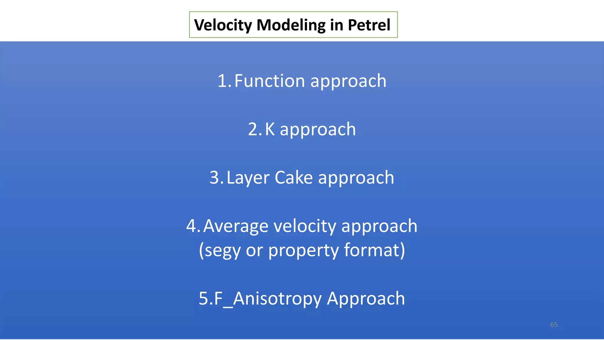
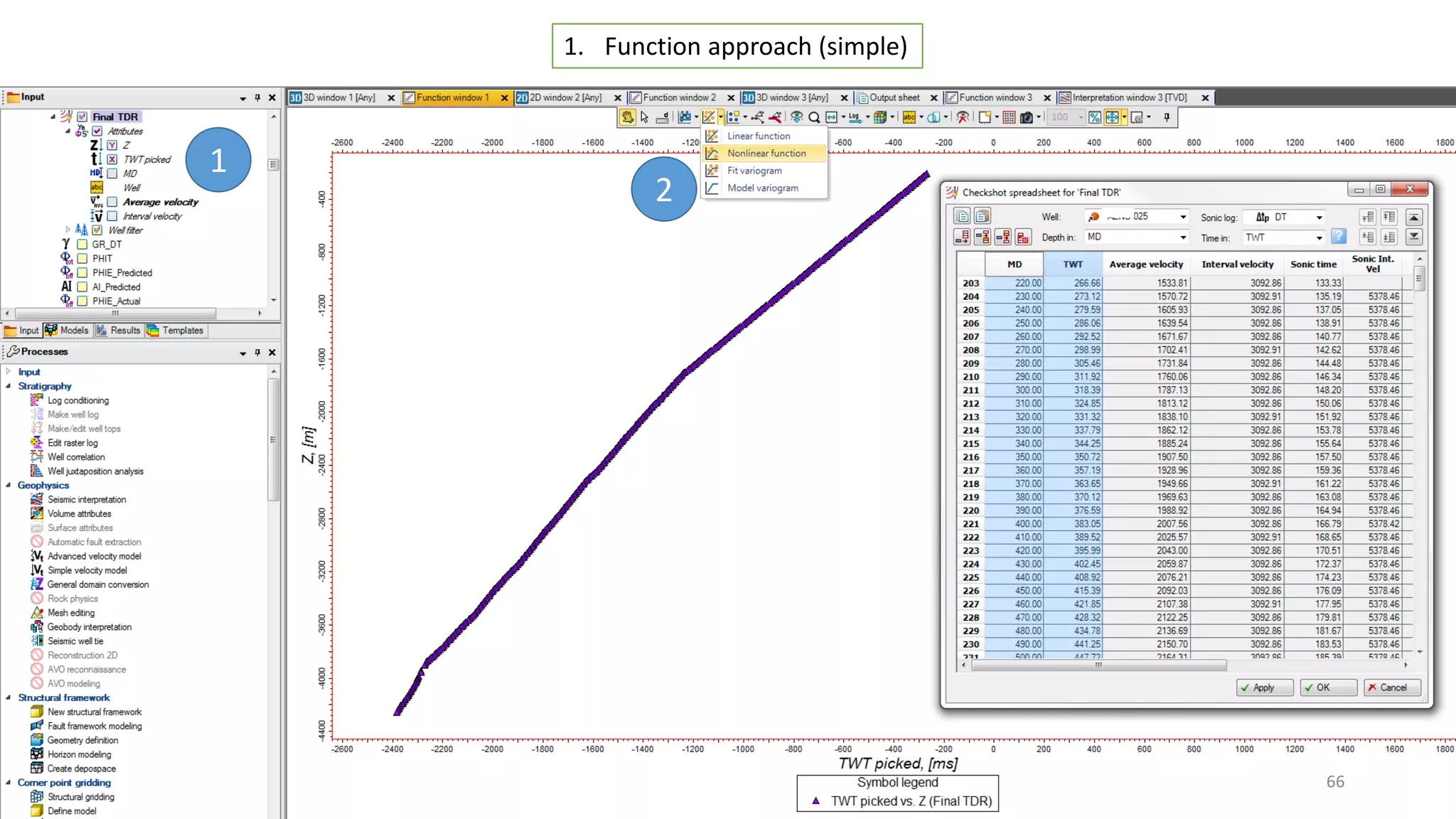
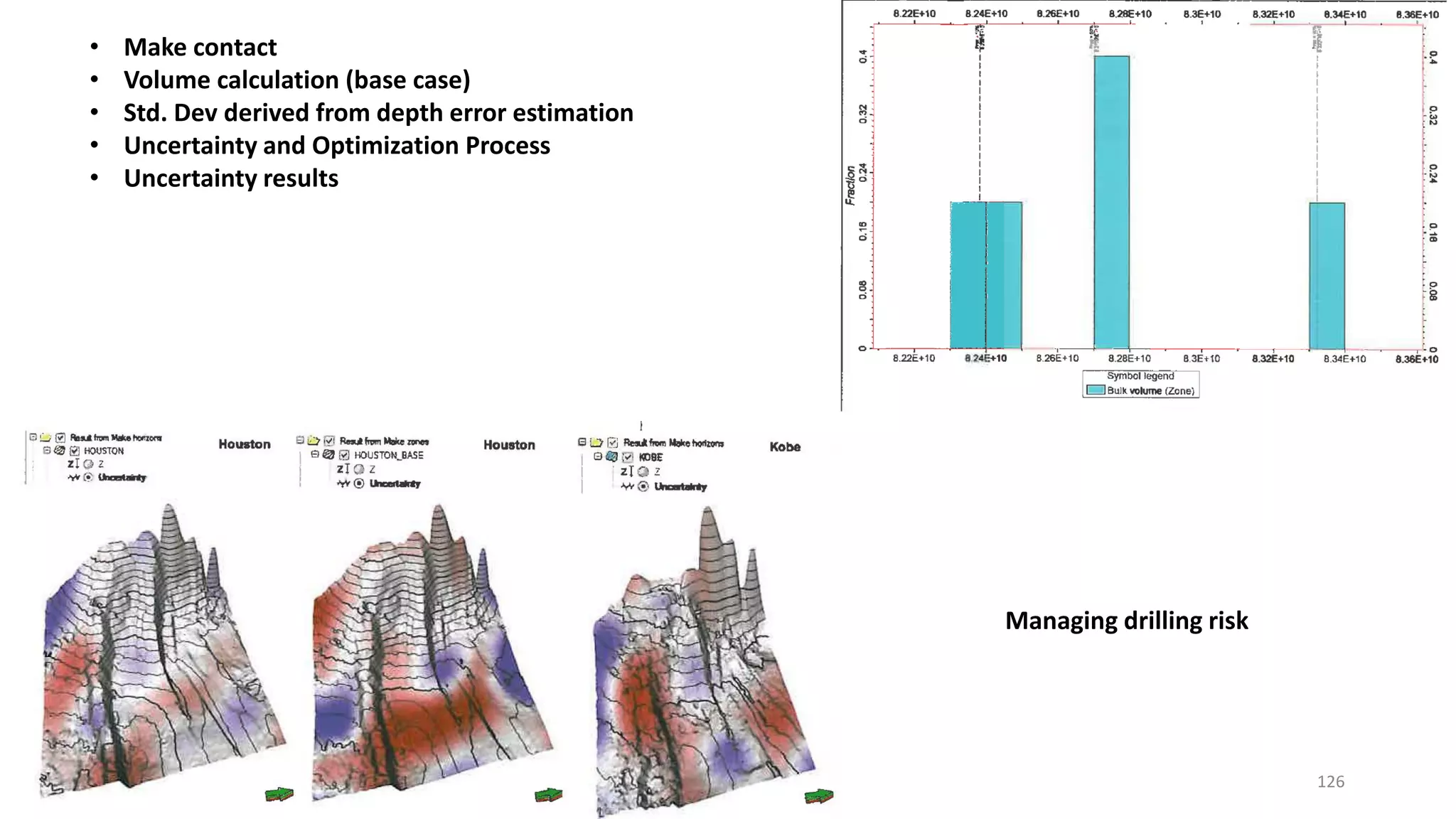
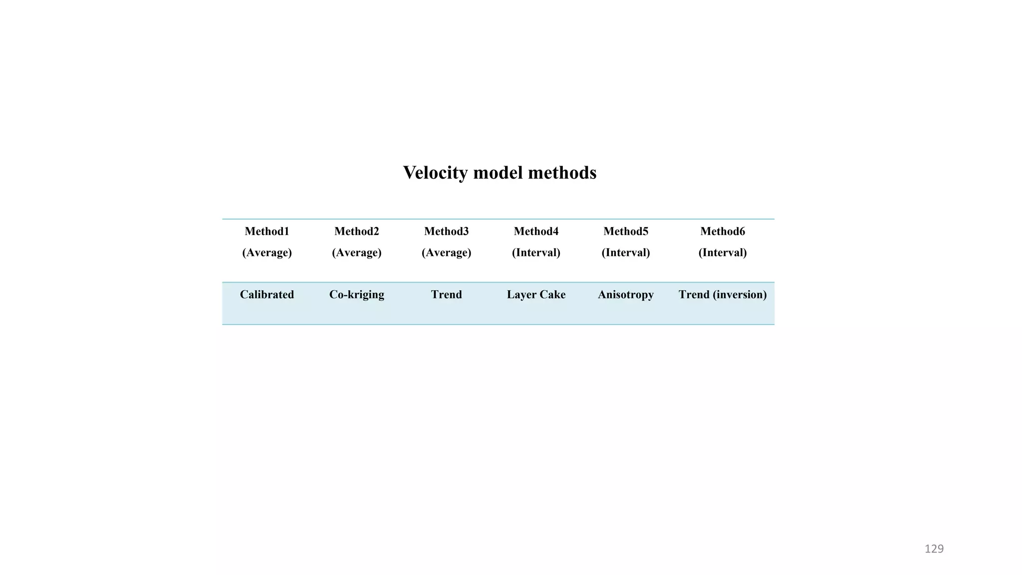
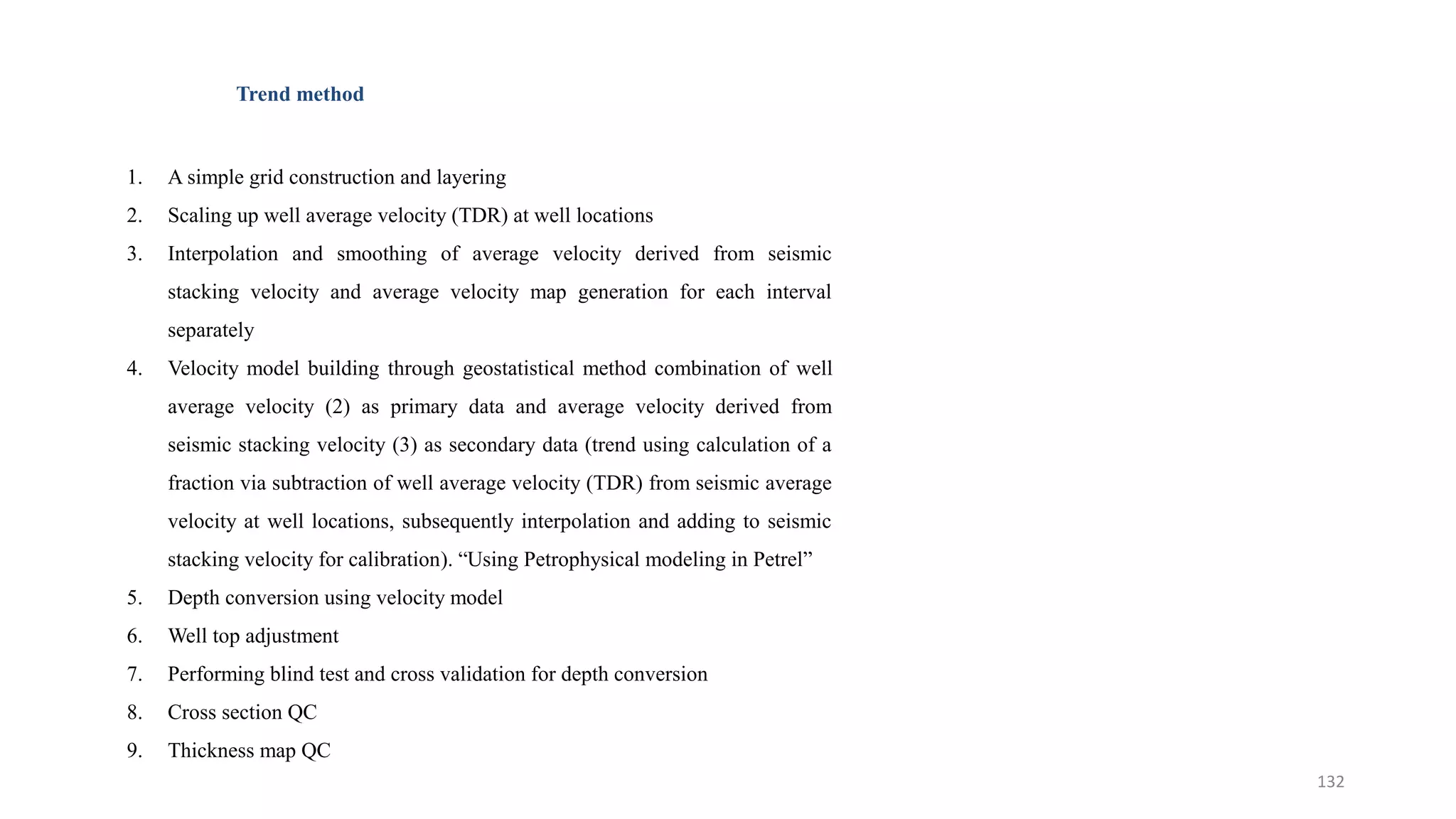
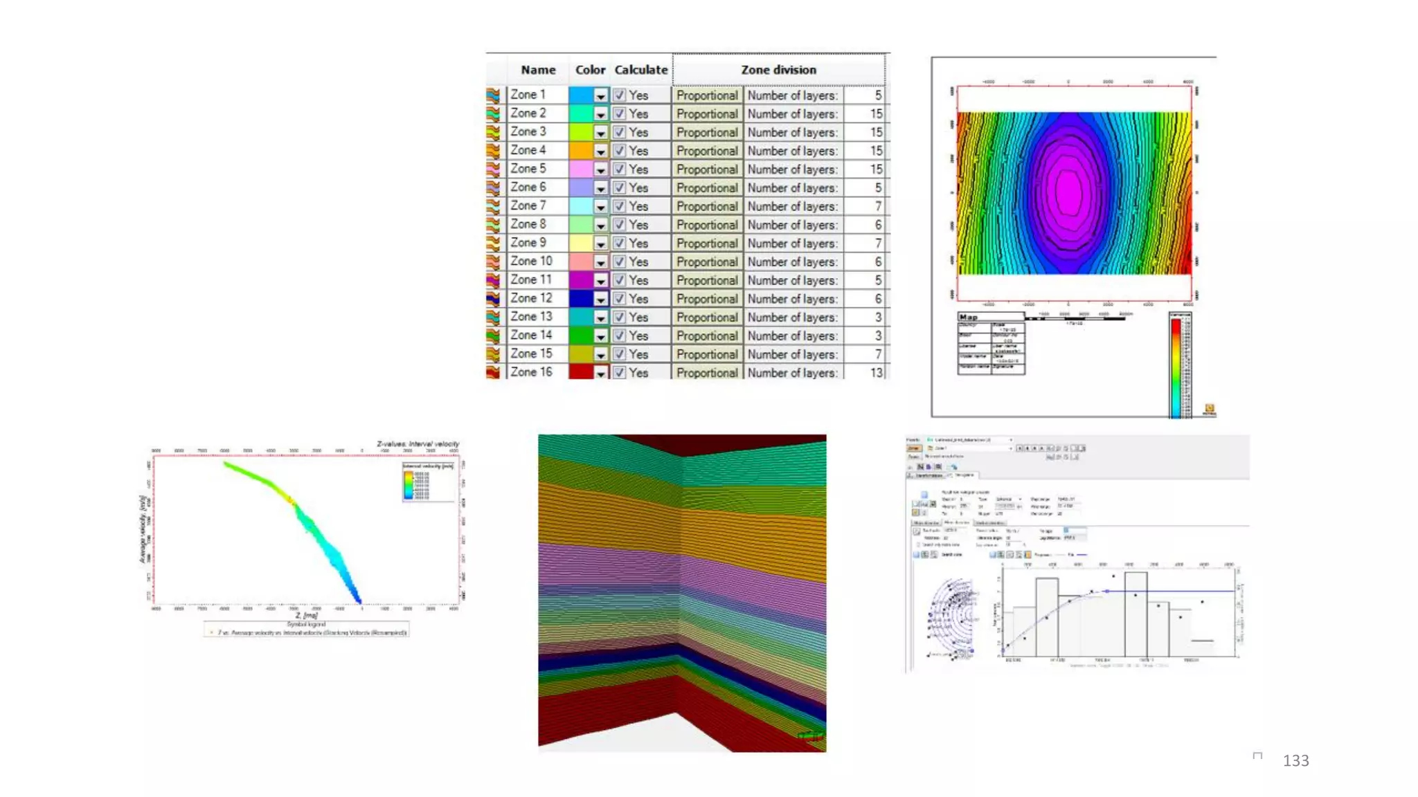
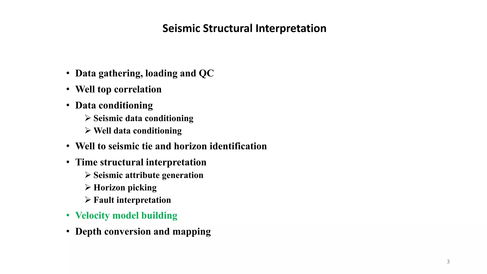
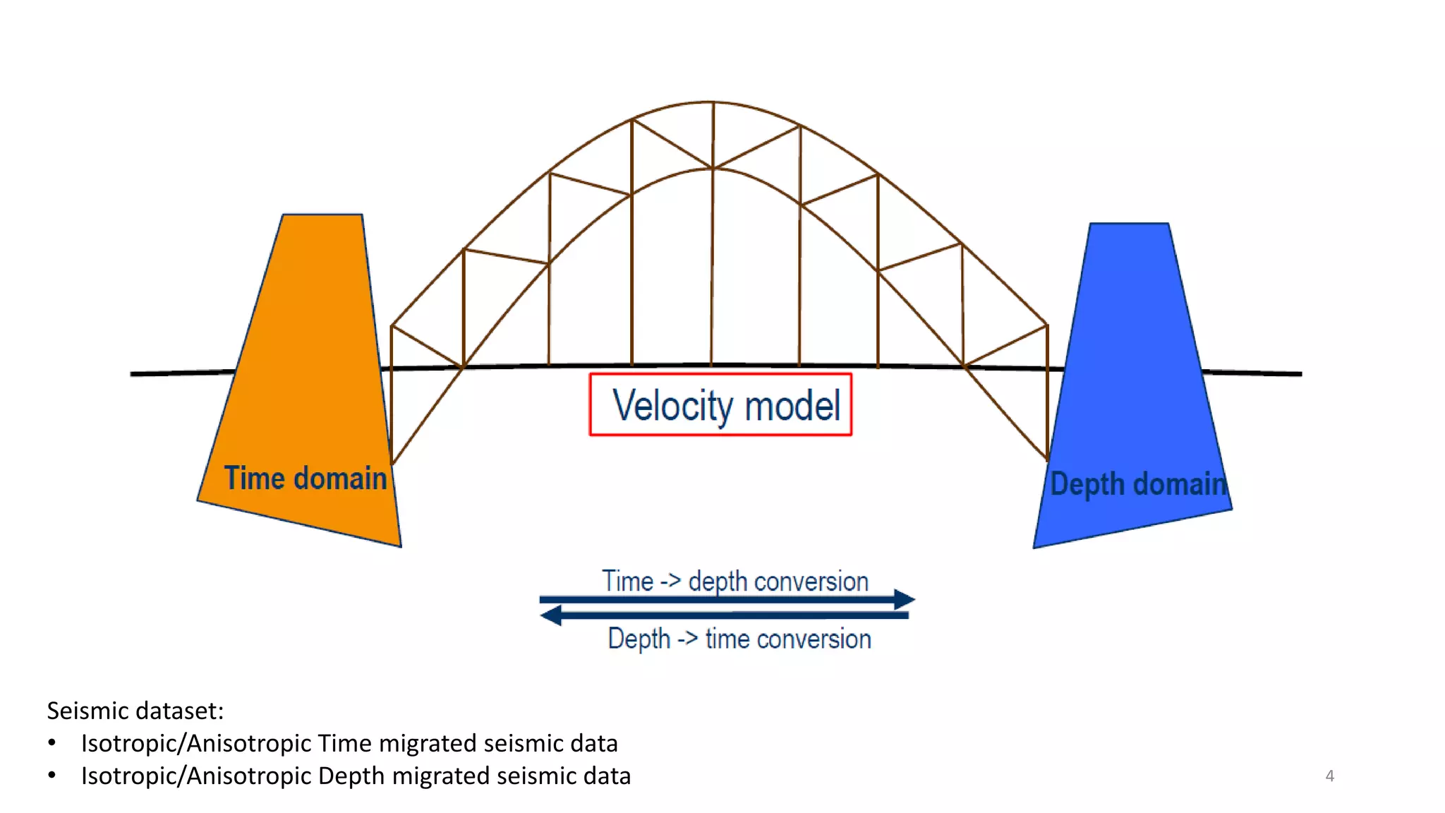
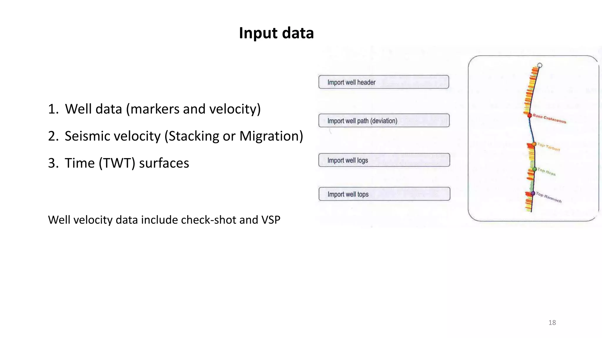
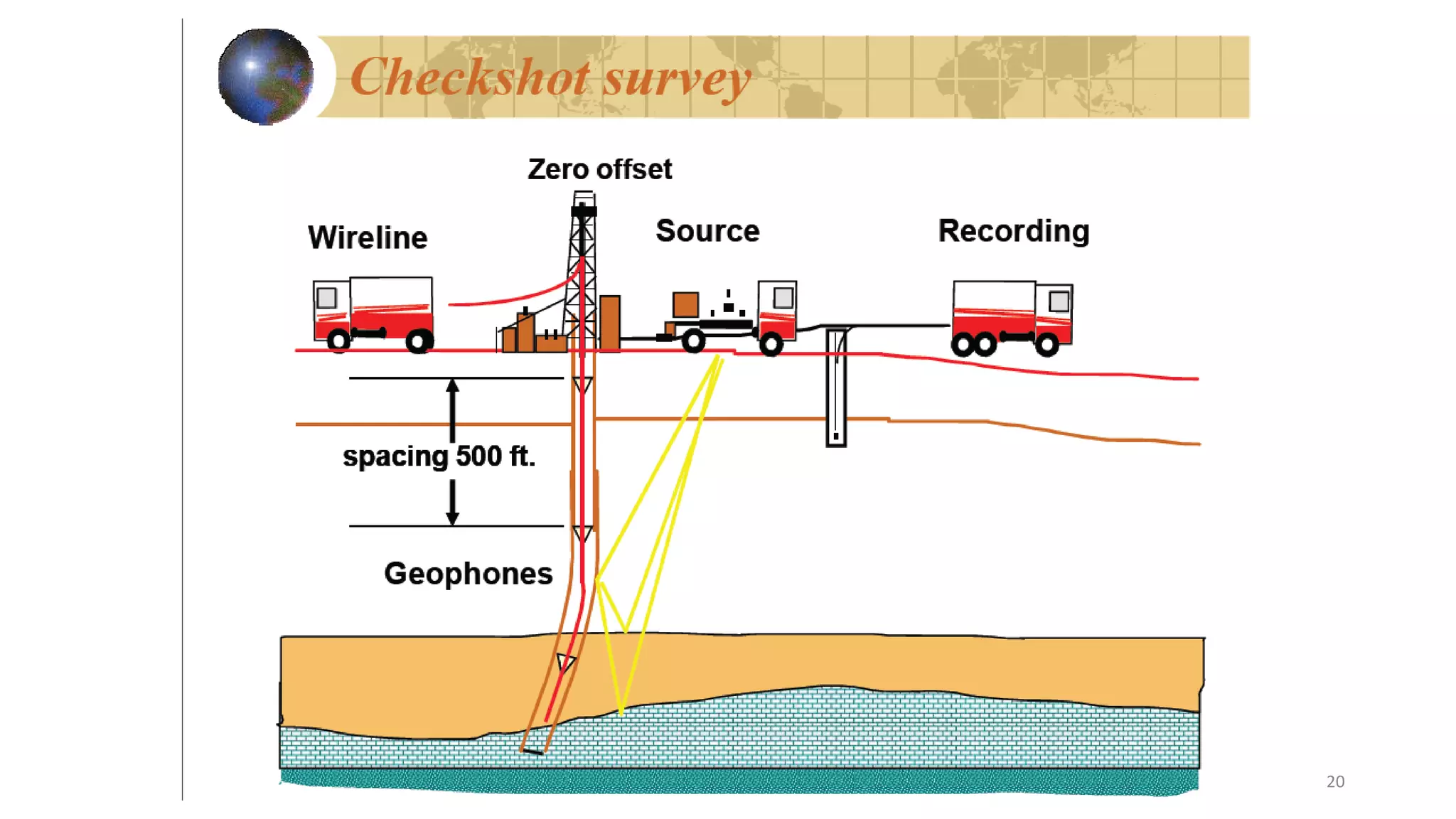
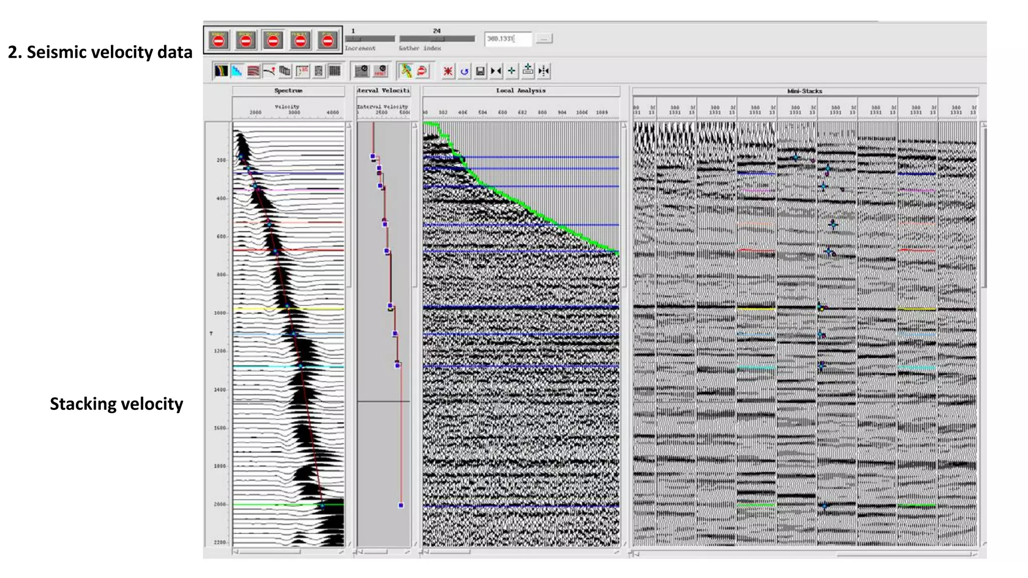
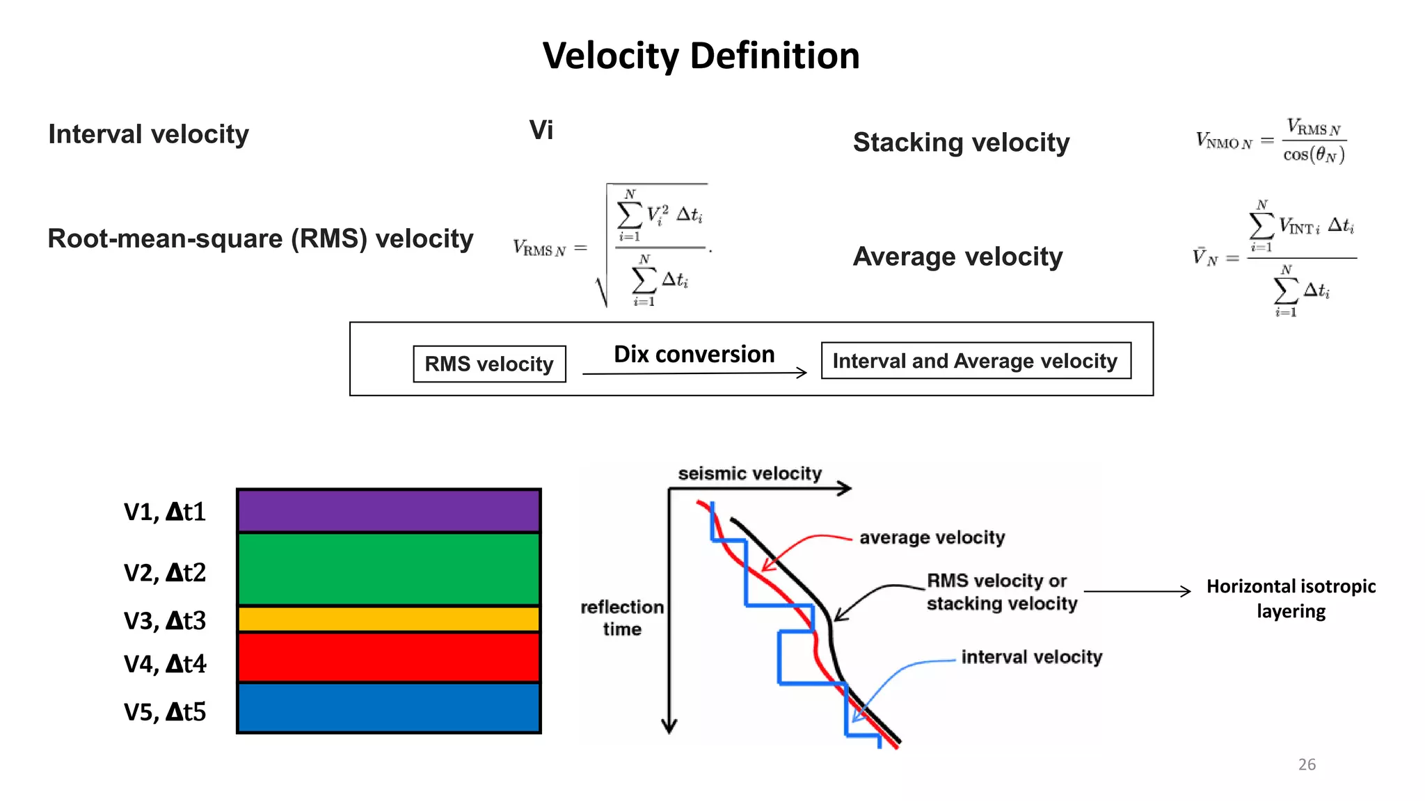
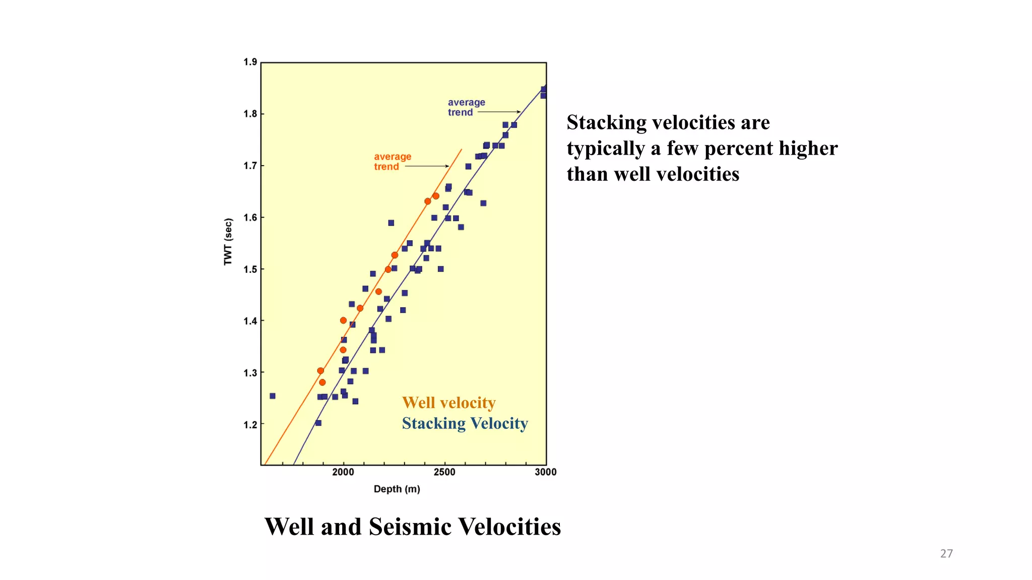
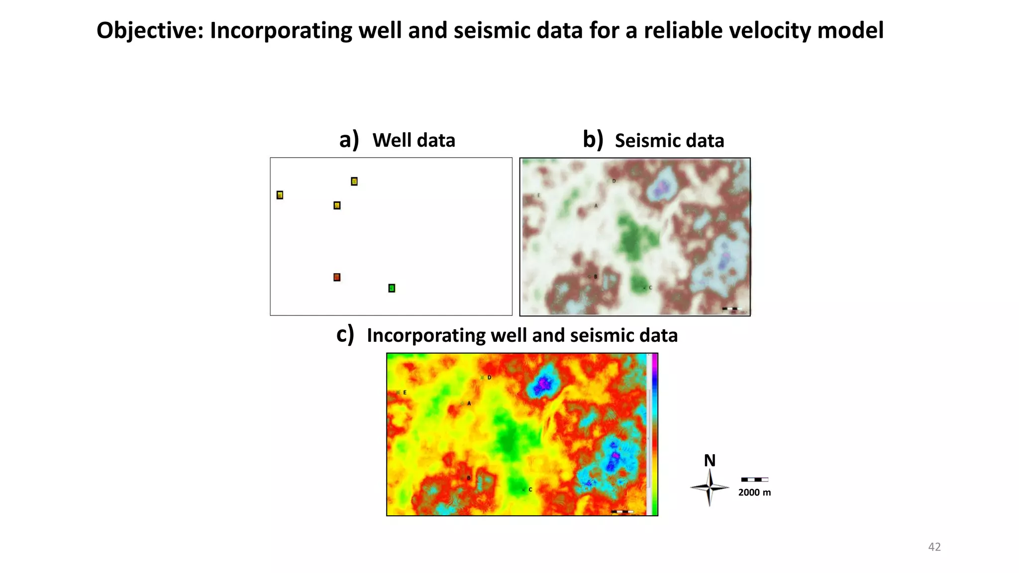
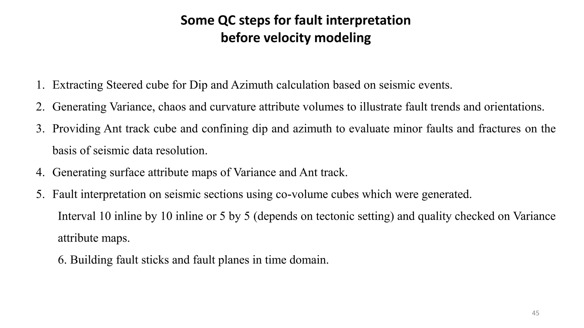
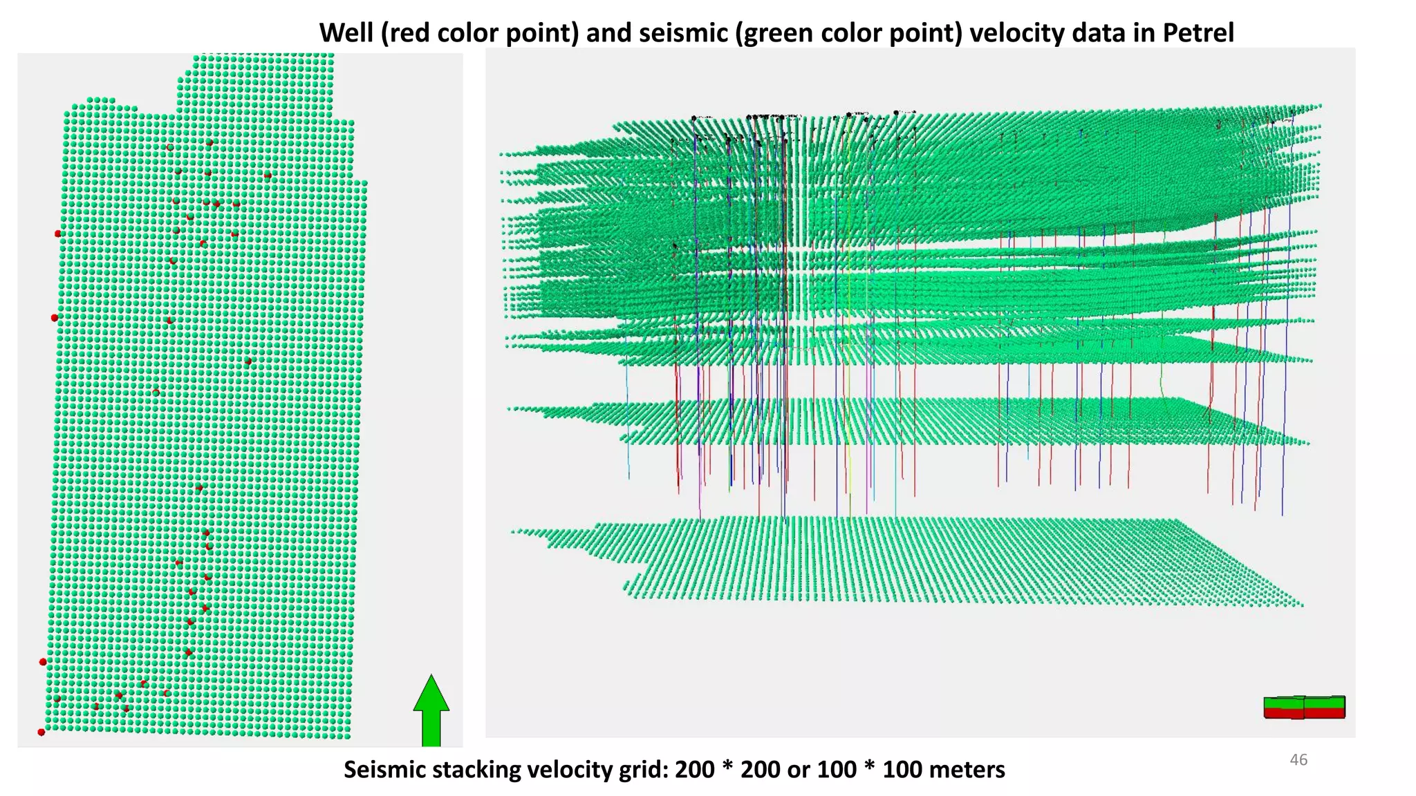
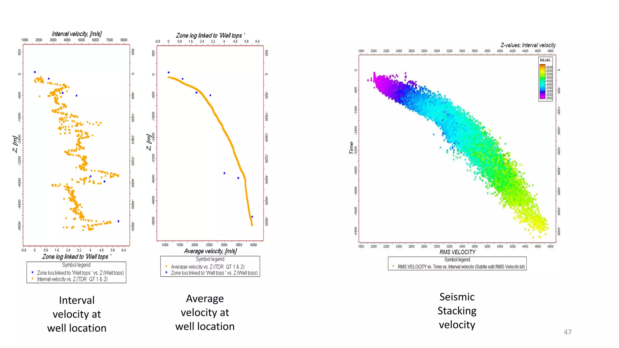
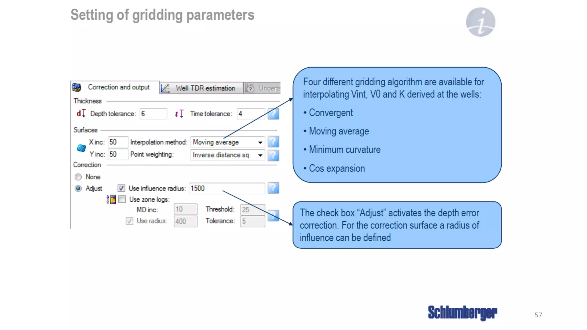
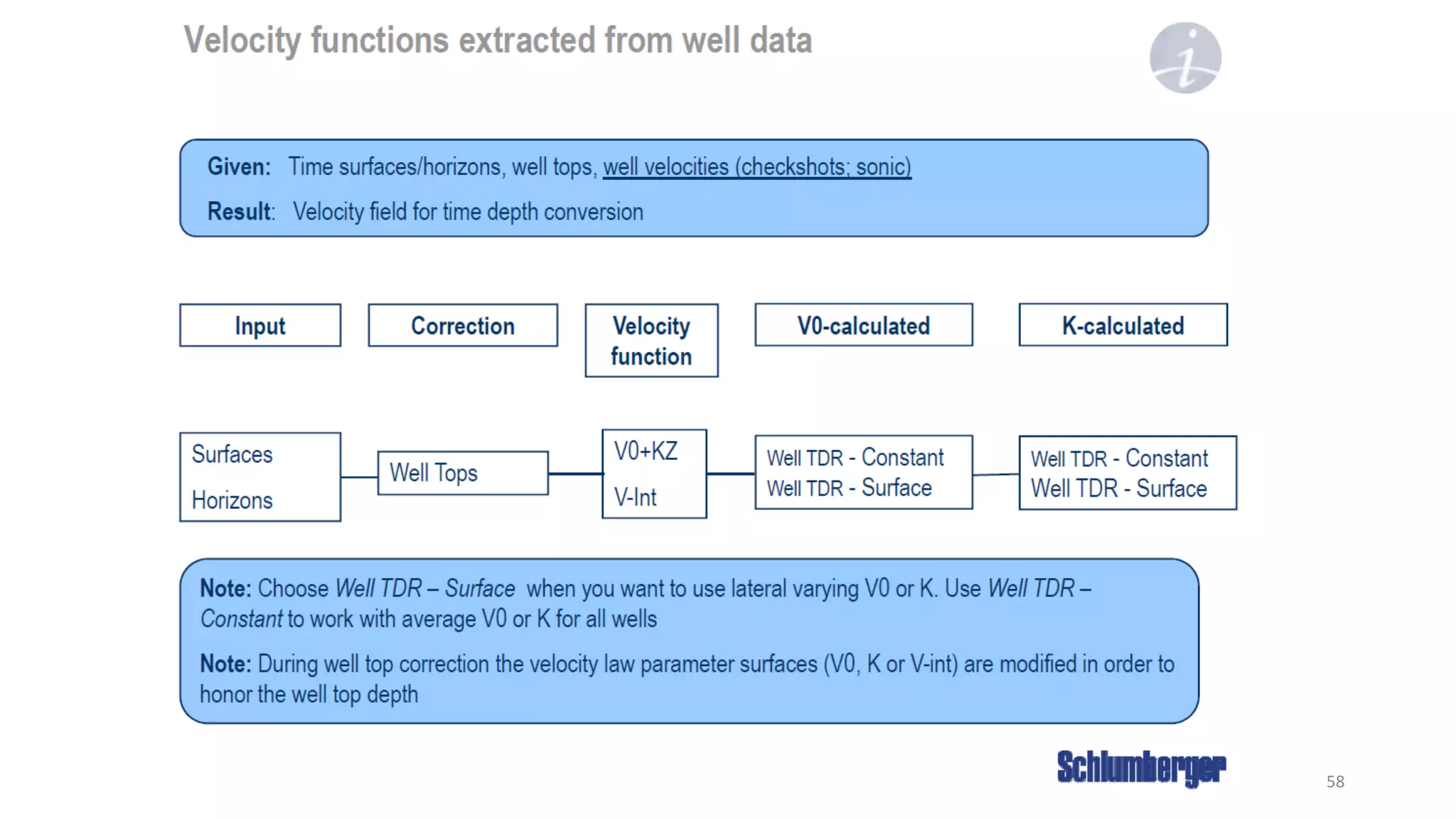
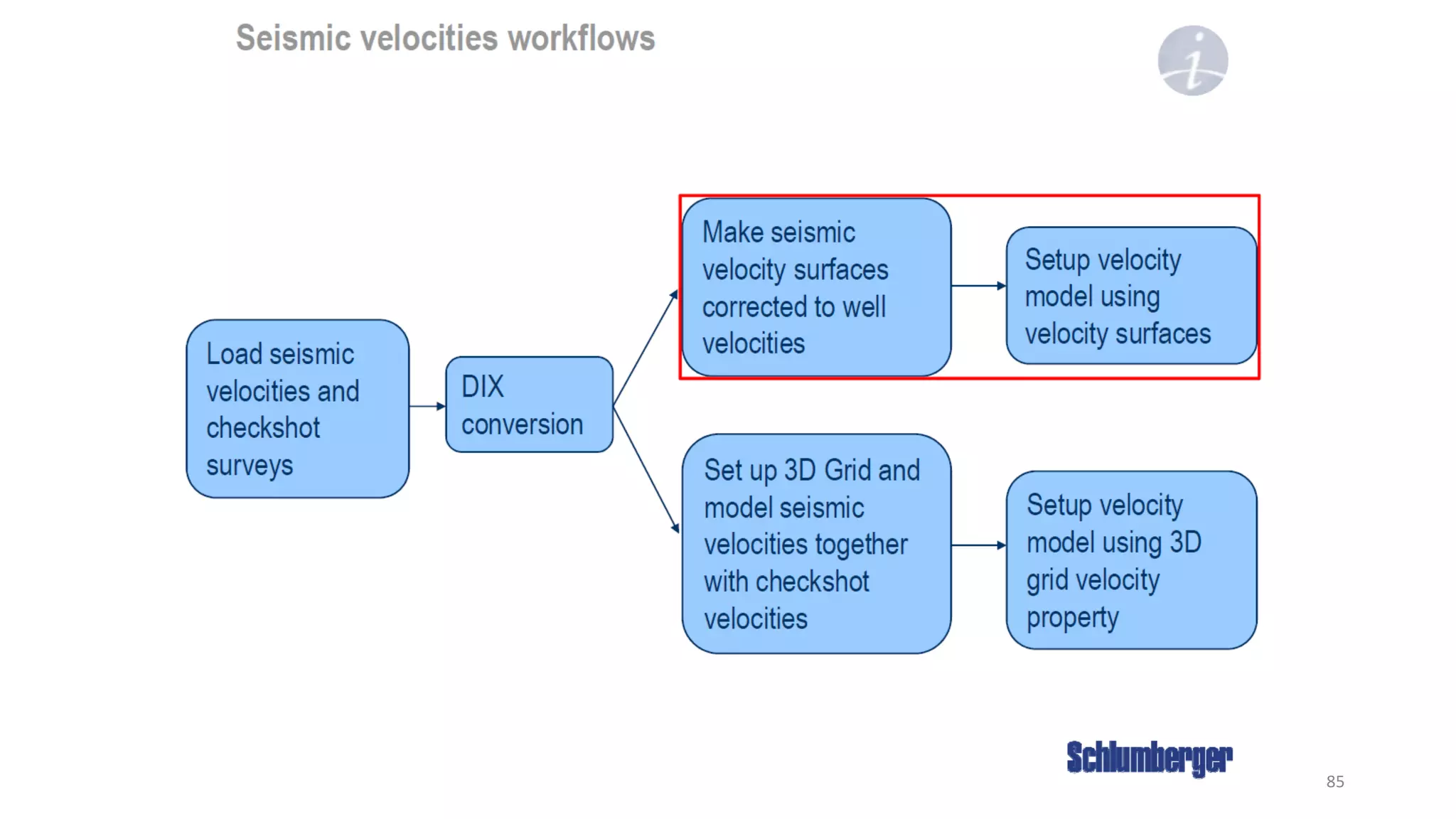
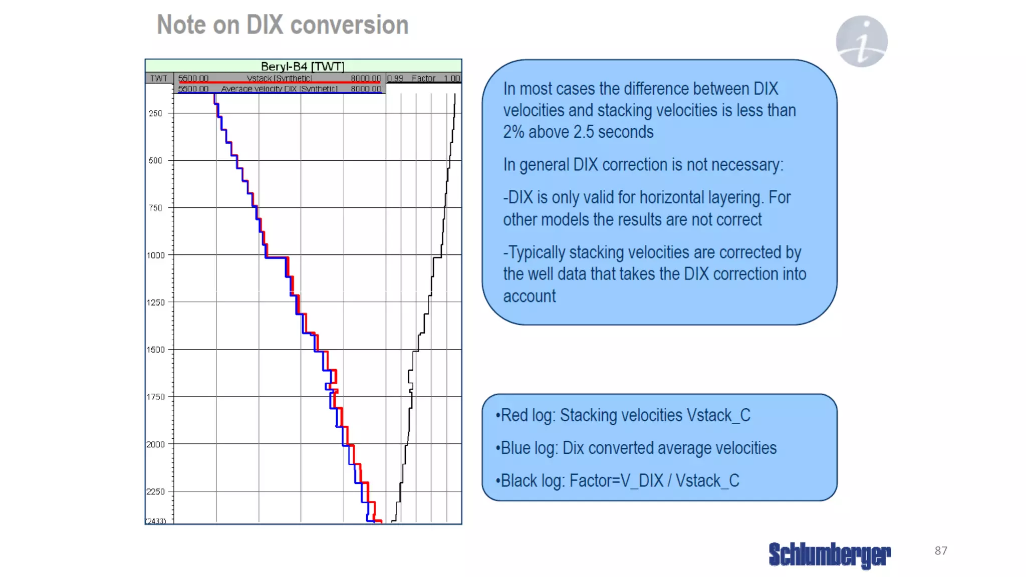
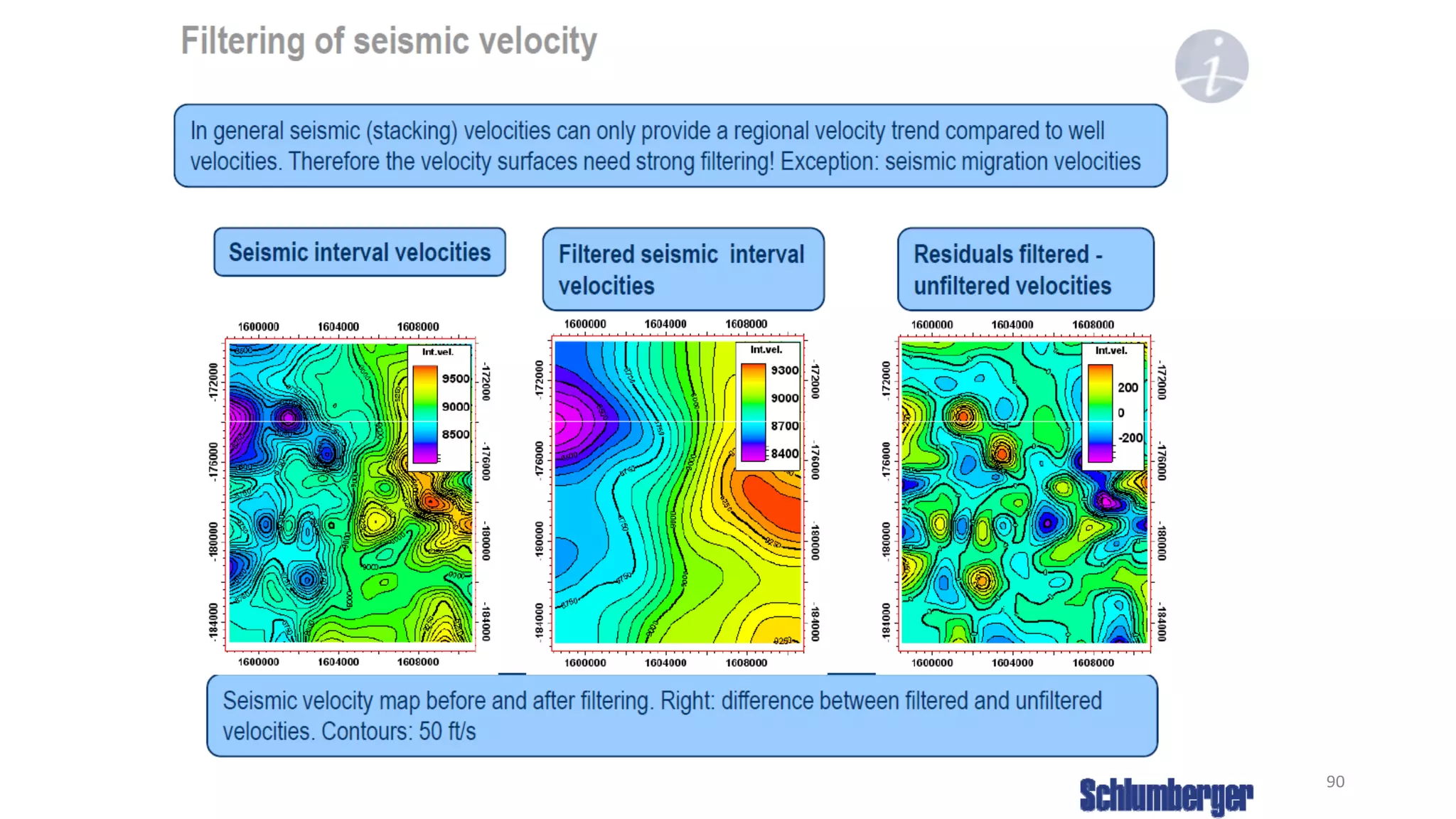
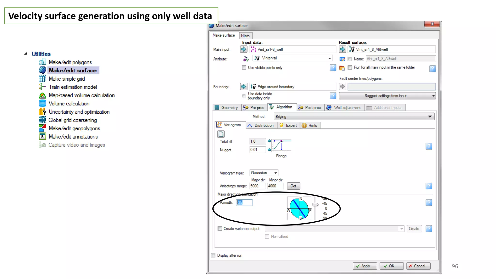
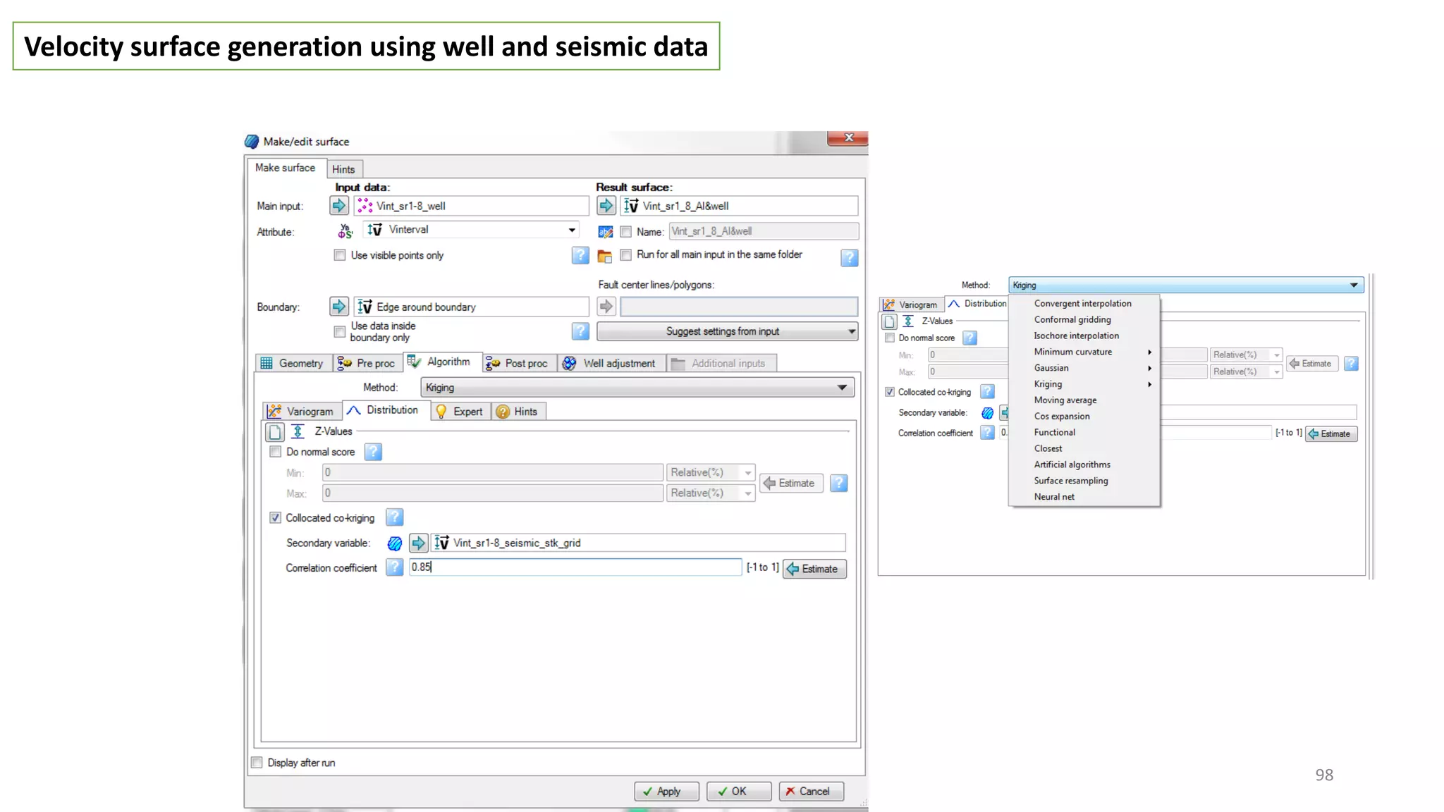
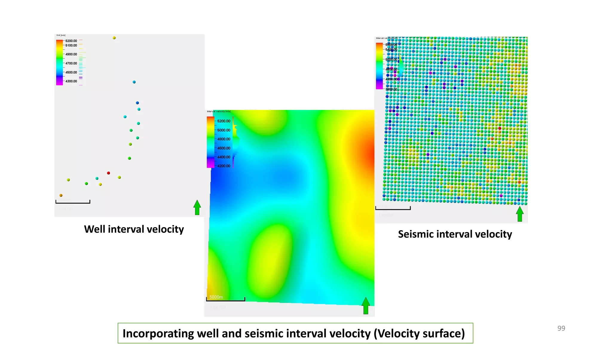
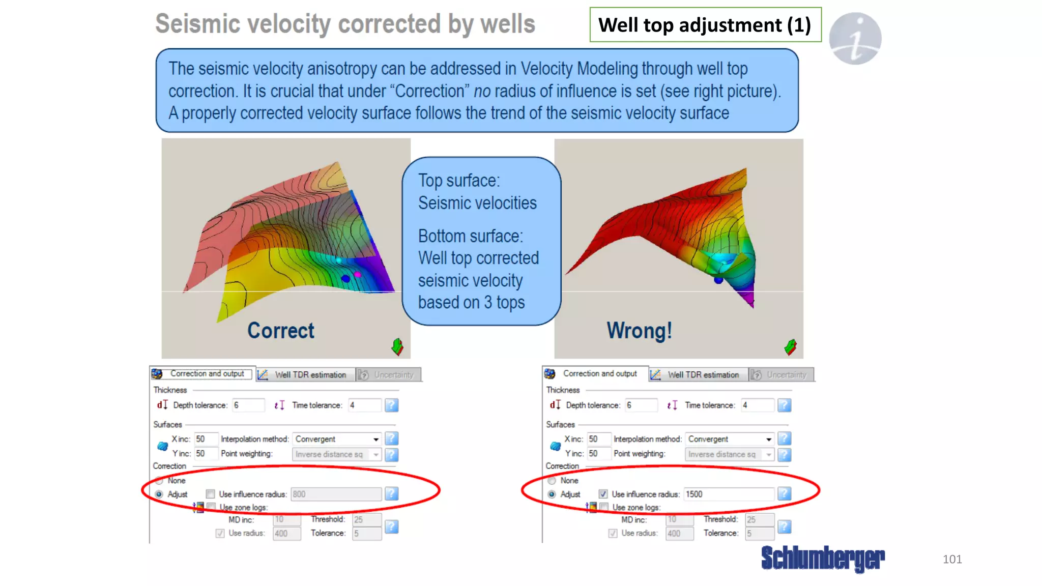
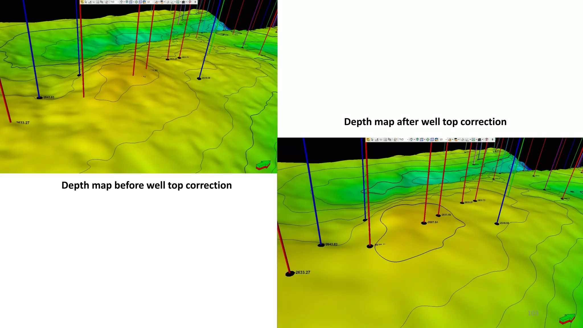
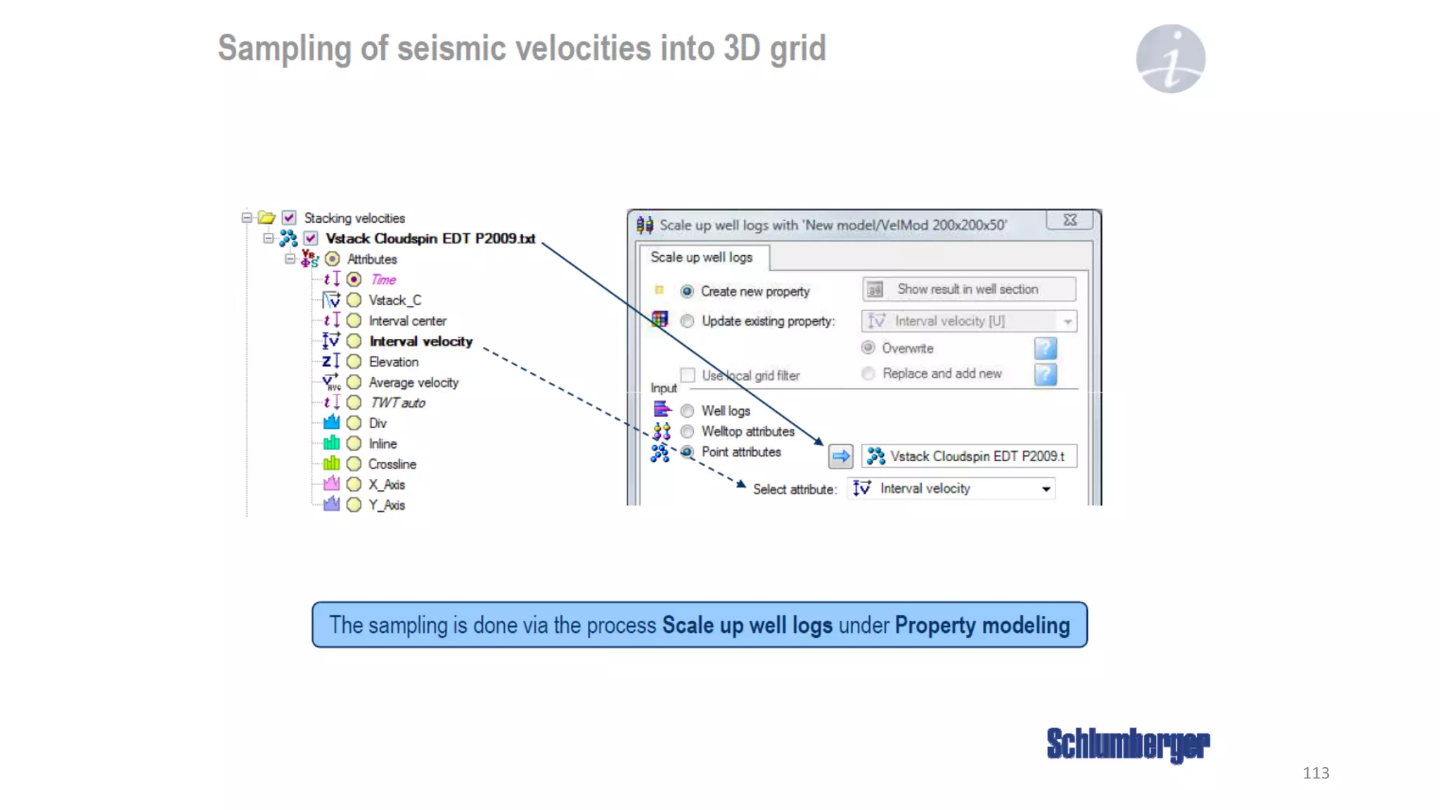
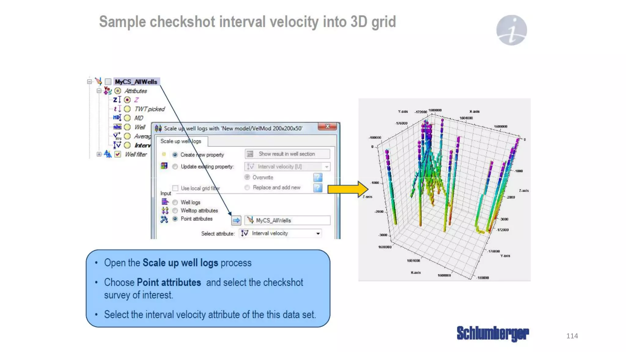
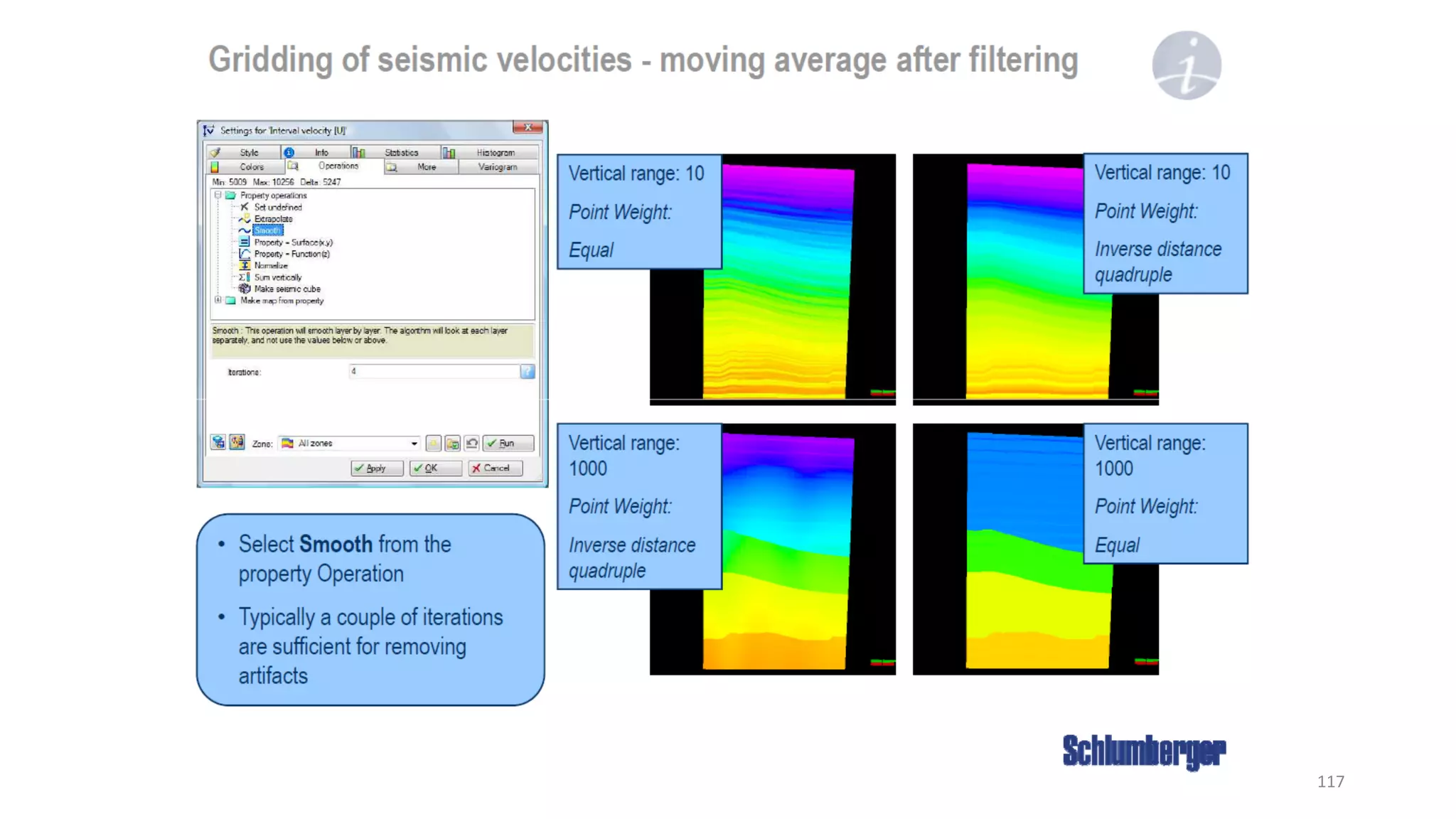
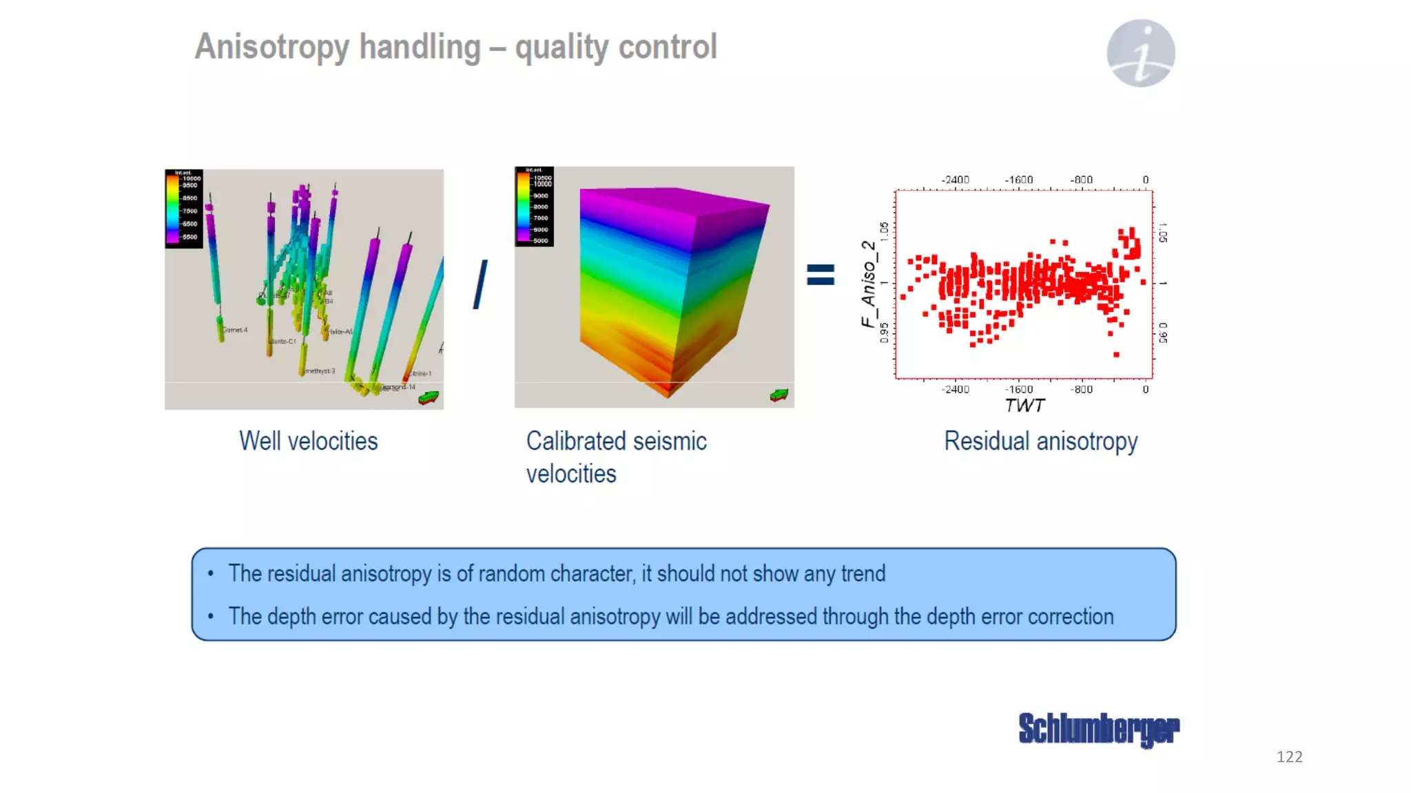
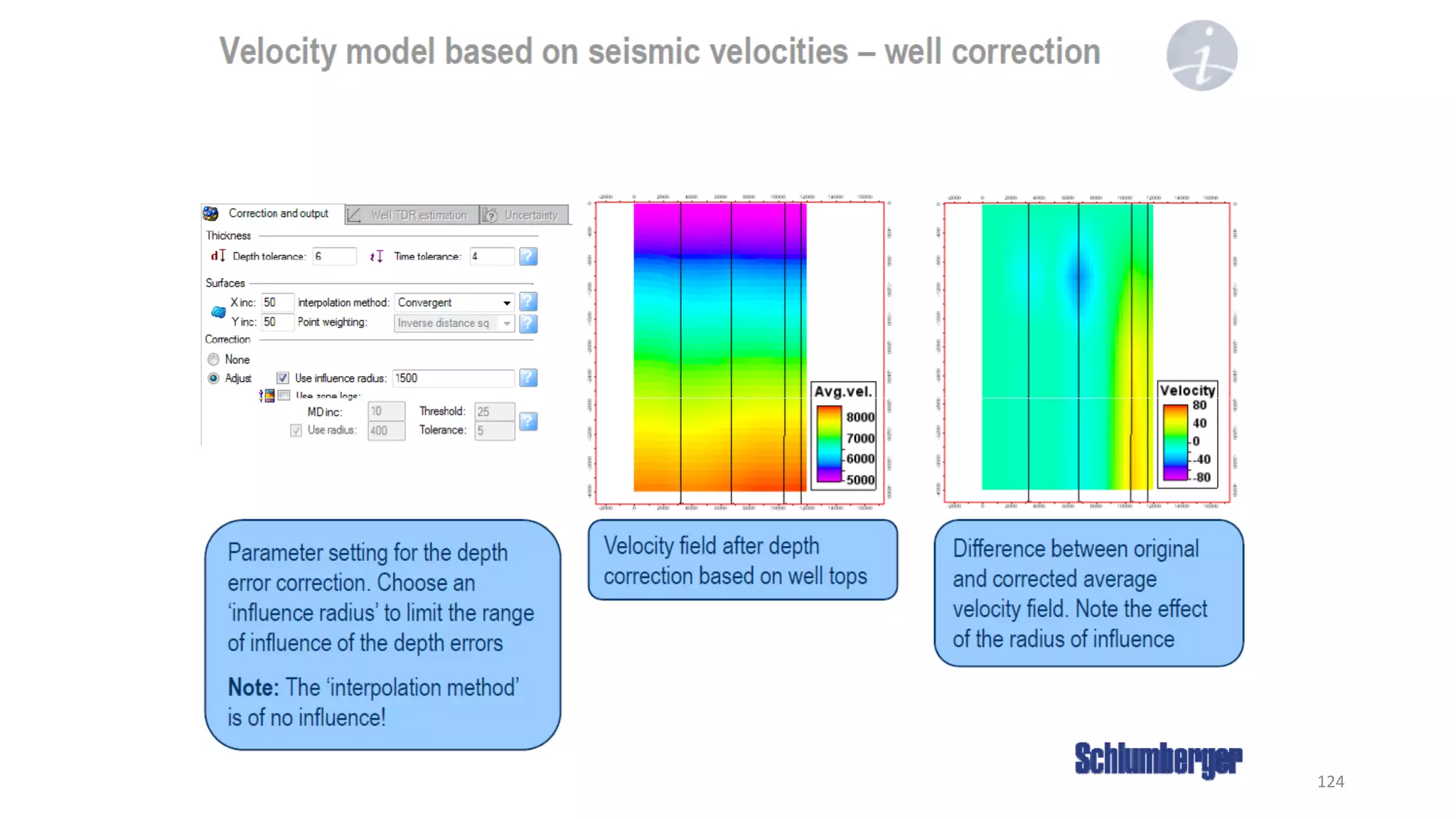
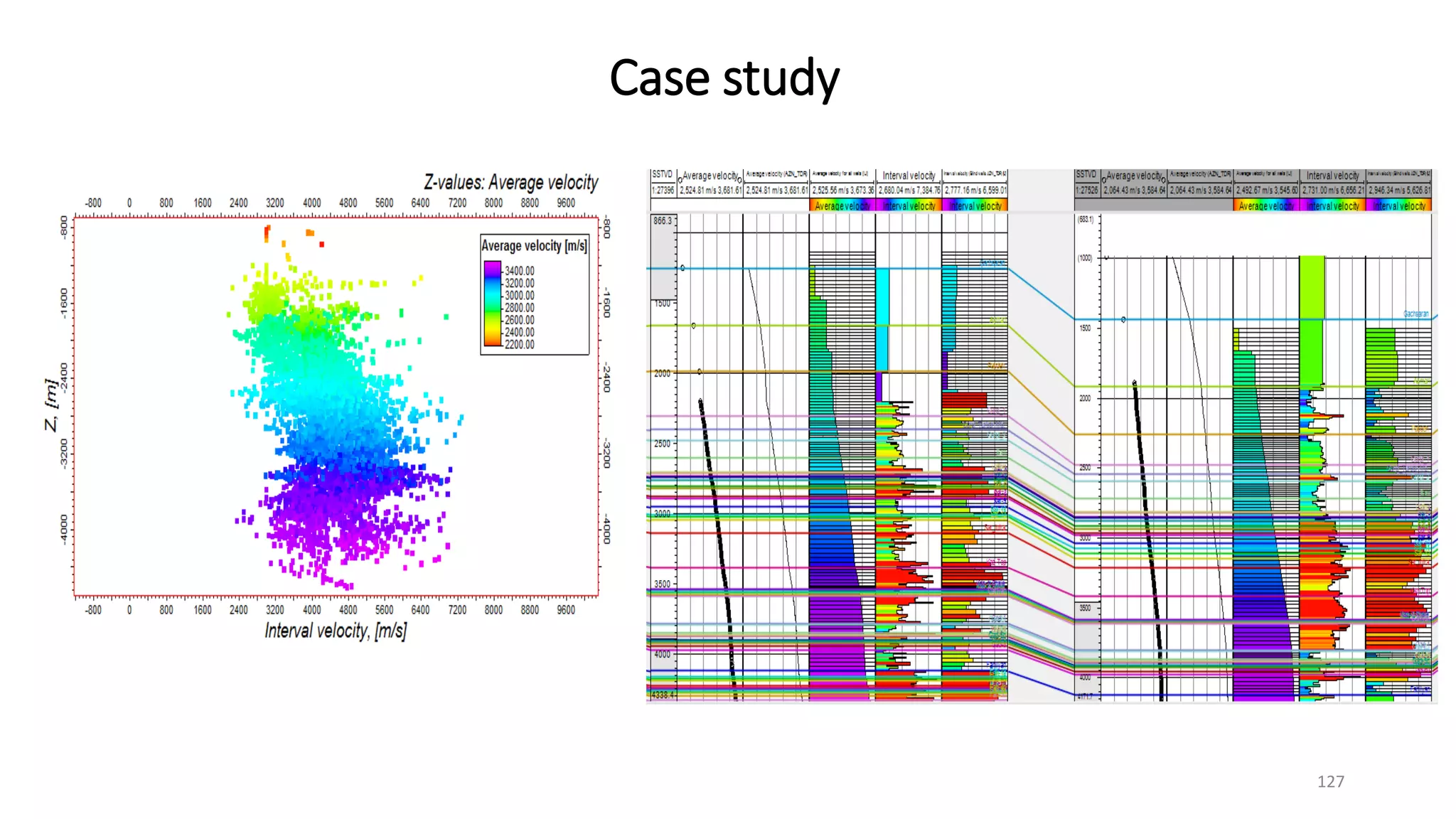
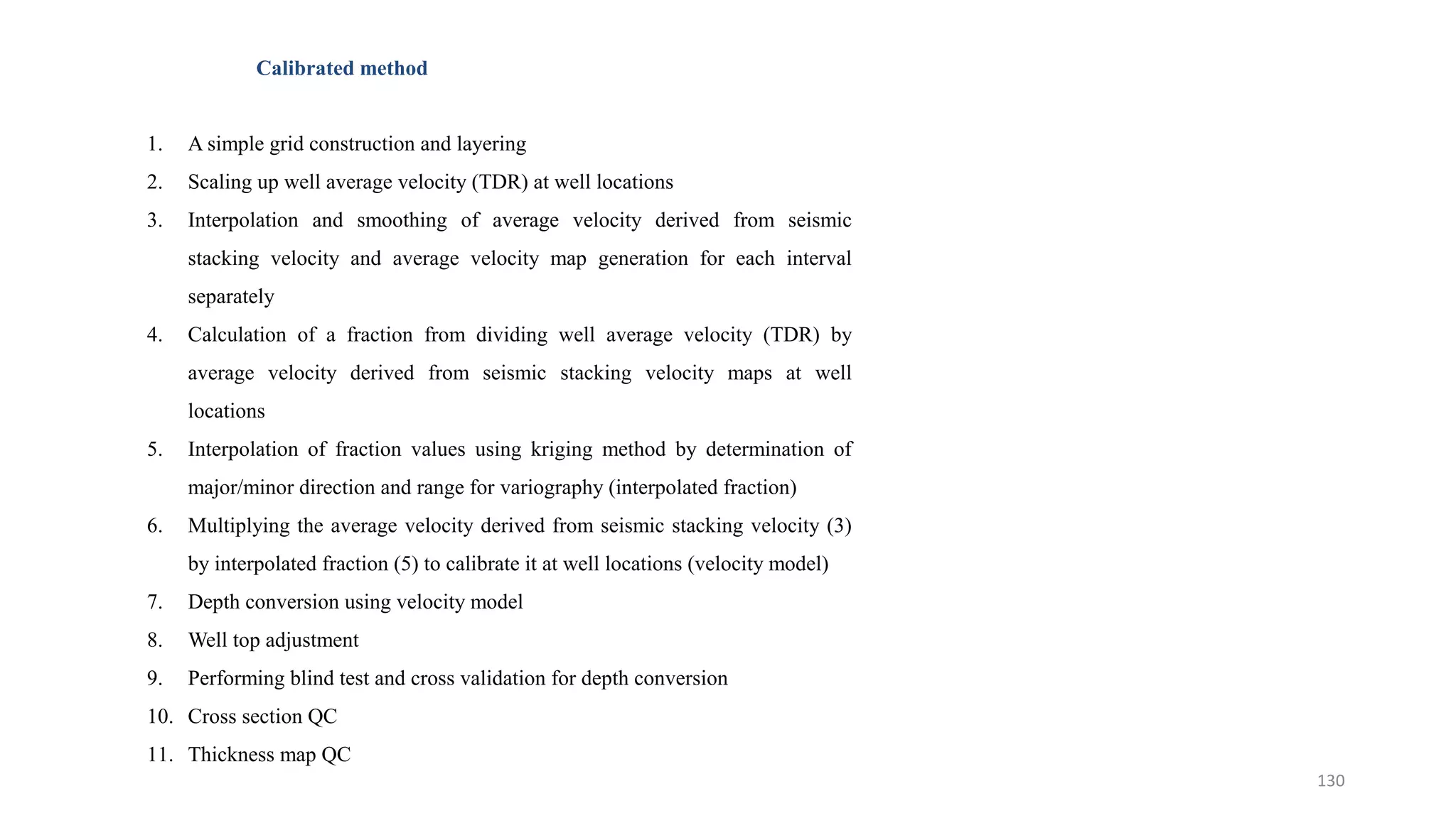
1. The document discusses various methods for building velocity models in Petrel software using well and seismic data, including average velocity, layer cake, and anisotropic approaches. 2. It provides steps for incorporating well velocity data, seismic stacking velocities, and time-depth curves to create interval velocity surfaces. Quality control steps are described for horizon and fault interpretation before velocity modeling. 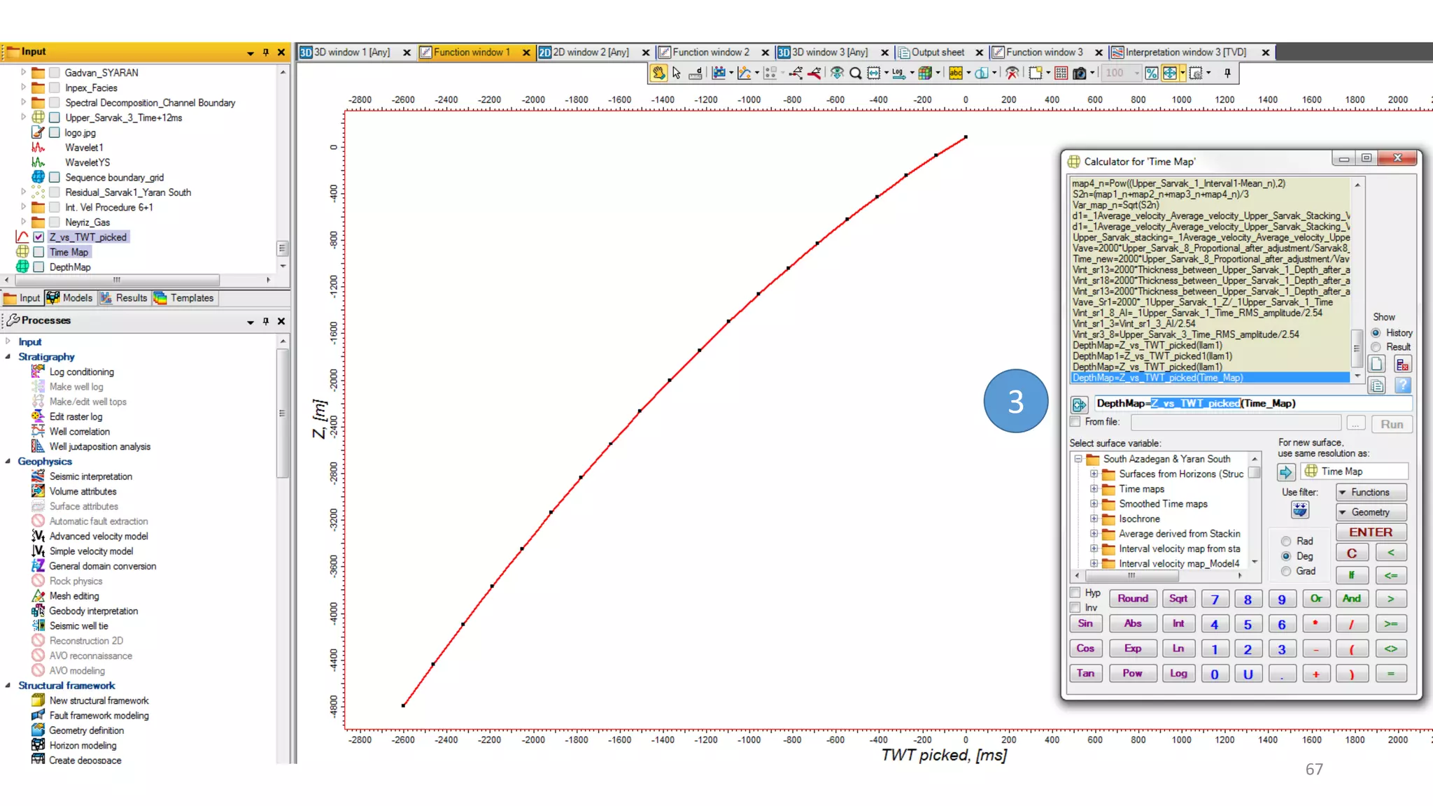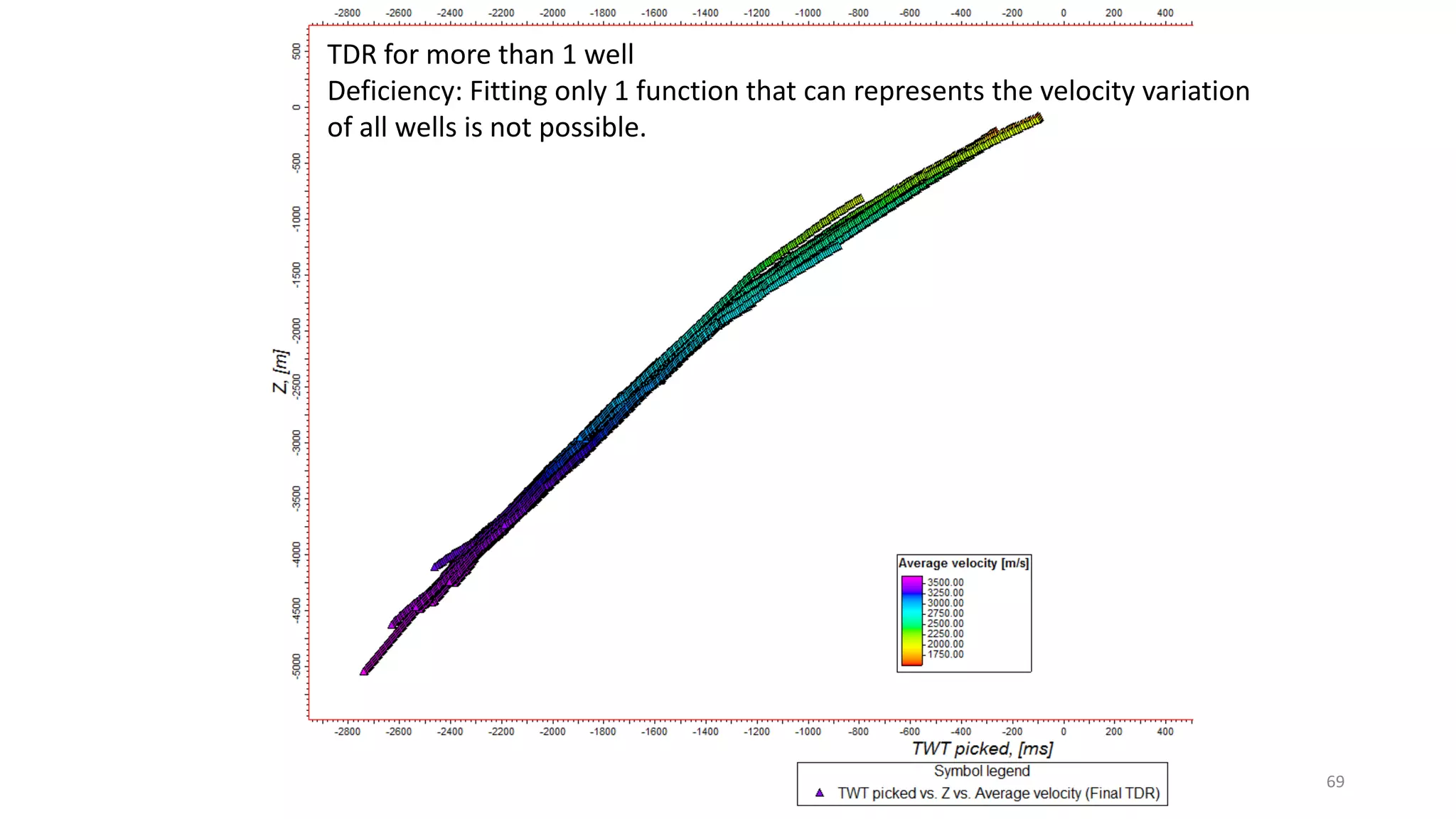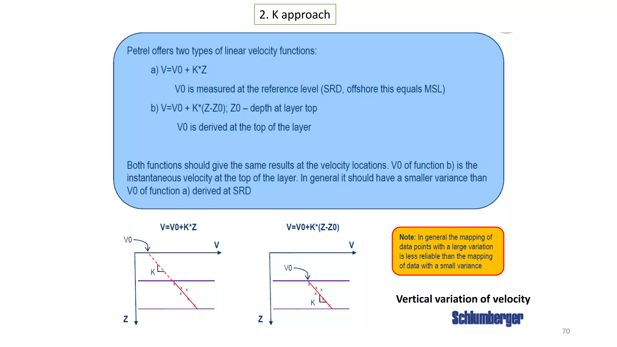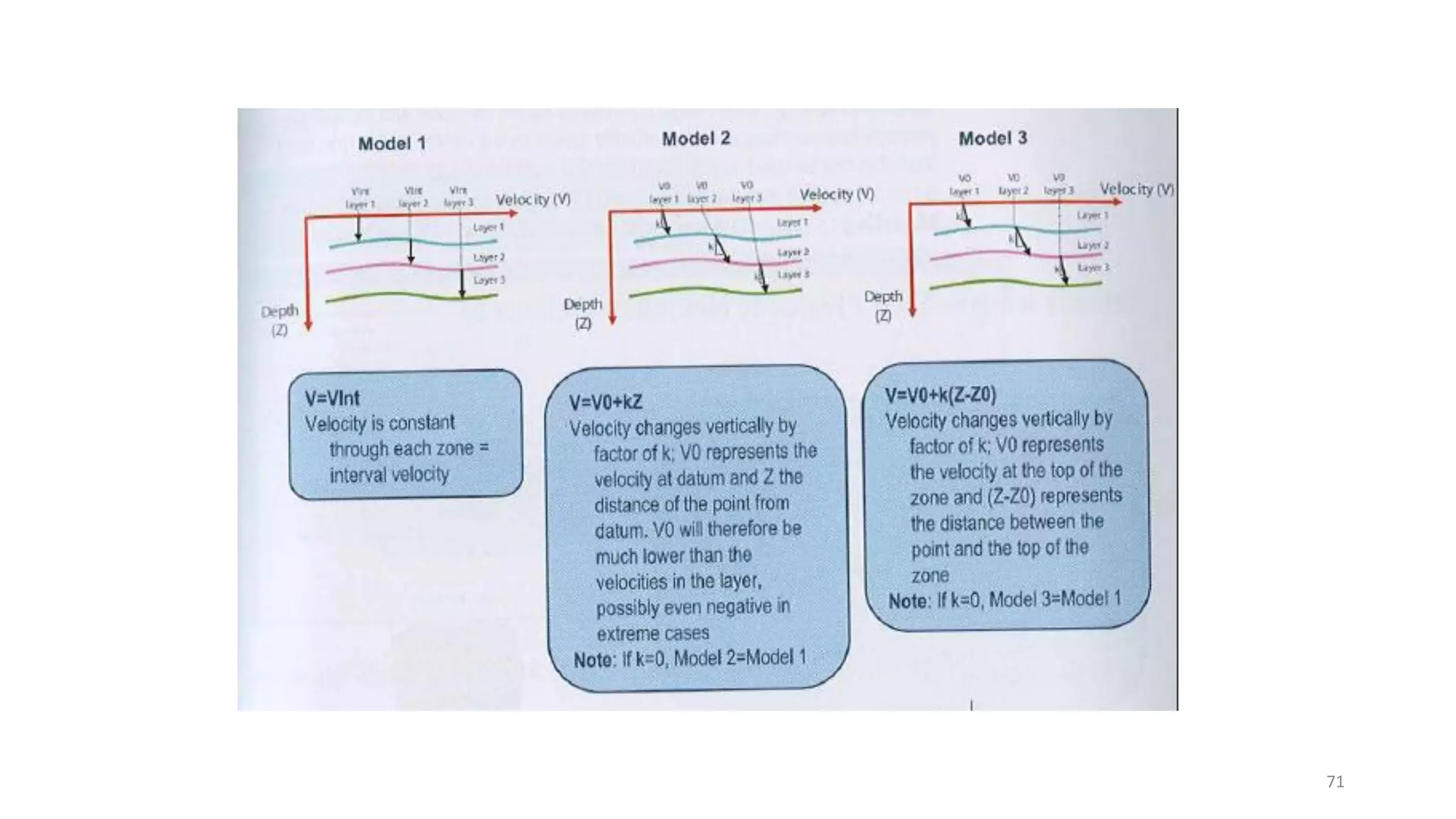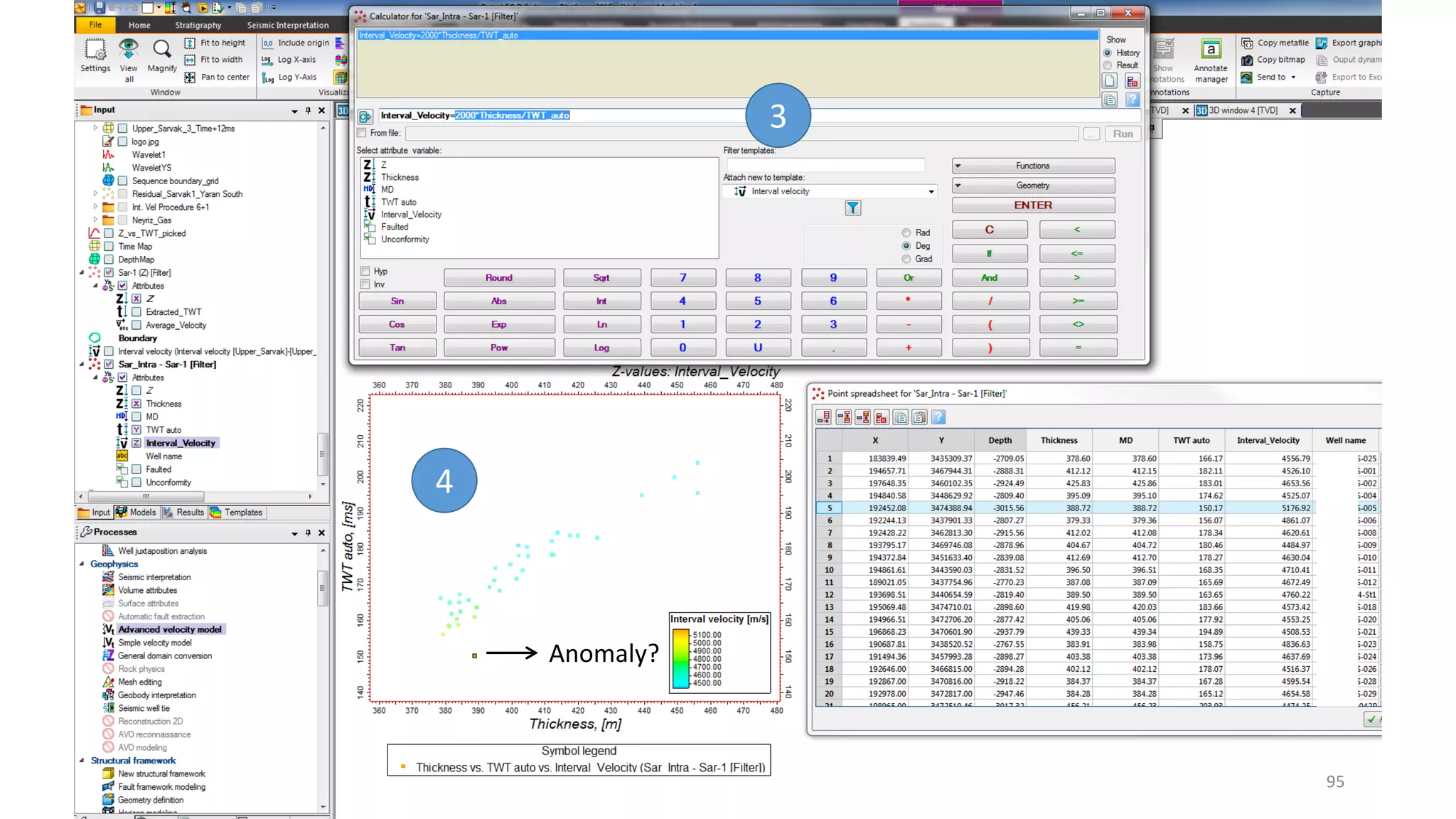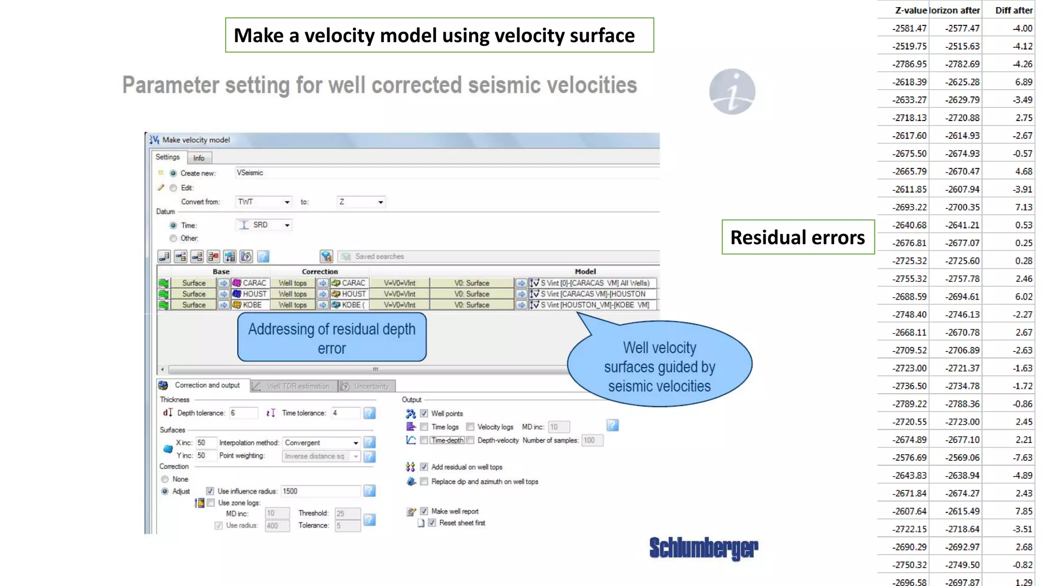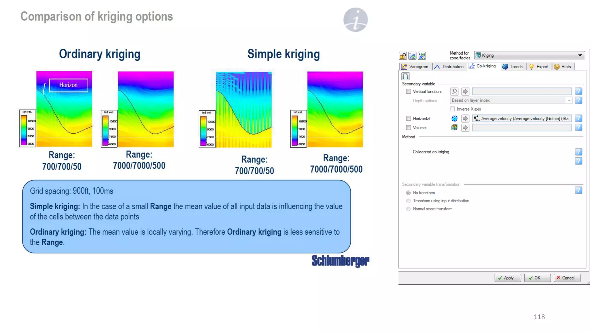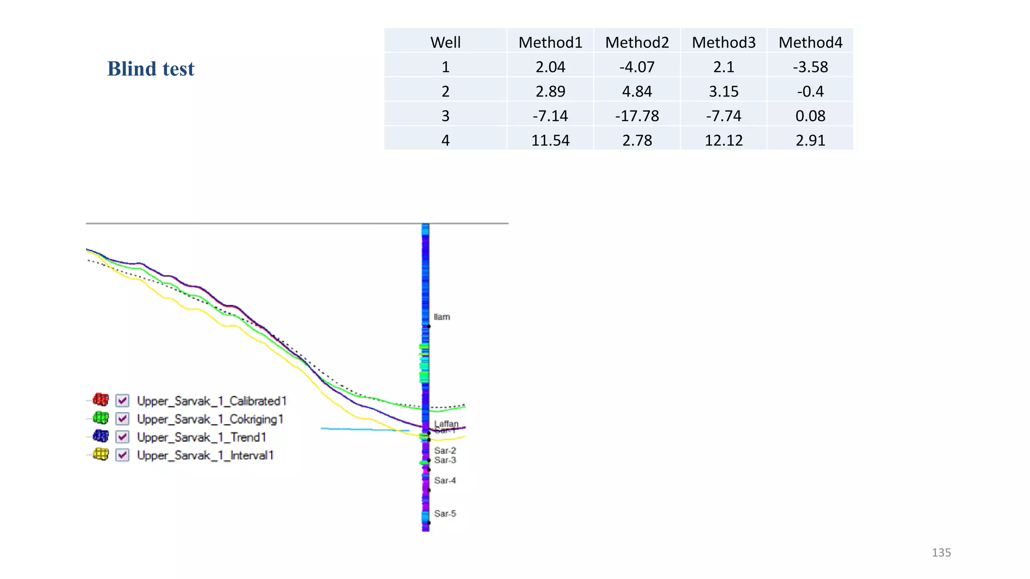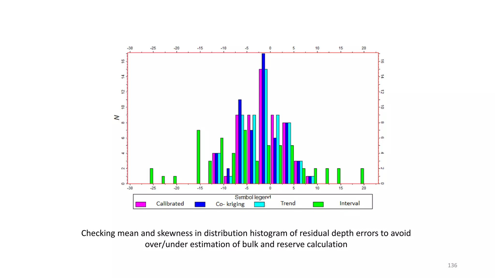3. Examples are given of different velocity modeling methods in Petrel and their applications, including calibrated co-kriging, trend modeling, and layer cake approaches. Metrics for evaluating velocity model accuracy like well tie errors are also discussed.

1. Velocity model building
using Petrel software
A
Universiti Teknologi Petronas
Centre Of Excellence In Subsurface Seismic Imaging
& Hydrocarbon Prediction (CSI)
Amir Abbas Babasafari
November 2019 1

2. Outline
• Velocity modeling the principles and pitfalls
• Well and seismic velocity data
• Incorporating velocity data to build a reliable model in Petrel software
• Time to Depth conversion (Map and reservoir property)
• Residual error correction and well marker adjustment
• Structural uncertainty
2
In this presentation some figures adapted from Dr. Badley, Dr. Robertson, Dr. Abdollahi far and Dr. Nosrat
and courtesy of Schlumberger, CGG, Jason and dGB.

3. • Data gathering, loading and QC
• Well top correlation
• Data conditioning
 Seismic data conditioning
 Well data conditioning
• Well to seismic tie and horizon identification
• Time structural interpretation
 Seismic attribute generation
 Horizon picking
 Fault interpretation
• Velocity model building
• Depth conversion and mapping
Seismic Structural Interpretation
3

4. Seismic dataset:
• Isotropic/Anisotropic Time migrated seismic data
• Isotropic/Anisotropic Depth migrated seismic data 4

5. Depth Conversion
 Geometric distortions due to velocity changes (pitfalls) will be removed
 To predict drilling depth to the target horizon
 More accurate Reserve Calculations and Uncertainty Quantification
 For basin modelling purpose
5

6. Pitfalls and issues in seismic data interpretation affecting seismic data quality and S/N ratio
Inherent : steep dip
fault zone
reflectivity
Acquisition : acquisition footprint
surface condition
navigation
receiver problem
shot problem
missed shots
recording problem
crooked line
feathering in marine
Processing : time mismatches
mute
polarity differences
vertical anomalies
static problem
filtering
Others : migration & sideswipe
display
tuning
velocity effects
multiples and bottom simulating reflectors
llimits of software packages 6

7. Common Velocity Pitfalls:
• Anomalous high/low velocity zone (lithology)
• Lateral lithofacies changes
• Fault zones
• Gas effect
7

8. 8
Seismic data acquisition
½ * Two-Way Time * Velocity = Depth

9. Velocity effects
Variations in velocity produce apparent structures which may not exist.
Velocity pull up
Velocity push down
9

10. Velocity effects and depth migration
Depth migration accounts for lateral variations
in velocity and can minimise the appearance
of spurious structures
Time migrated section
Depth migrated section
10

11. 11
Drastic lithology changes
Lateral lithofacies changes

12. Fault shadows
A subtle form of velocity effect can
produce not just spurious folds but
also apparent faults
12

13. Velocity Distortion
Increasing velocity downdip
- the interval appears to thin
13

14. Distortion of Structure
on Time Sections
DEPTH
TIME
Planar faults appear
Listric
Uniform thickness
beds appear to thin
with depth
14

15. Time and Depth Sections
Salt Layer – 4600m/s
15

16. Depth Conversion
Time section
Note that the water depth increases from 100m on the
right to 2.2km on the left
Depth section
The prospect is now imaged as a structural closure. The rapid lateral variations in
water depth and overburden are responsible for the distortion of the time section.
Prospect
16

17. Velocity push down
due to gas cloud
17

18. 1. Well data (markers and velocity)
2. Seismic velocity (Stacking or Migration)
3. Time (TWT) surfaces
Well velocity data include check-shot and VSP
18
Input data

19. 19

20. 20

21. 21

22. 22

23. Time-Depth Curve
0
500
1000
1500
2000
2500
3000
0 5000 10000 15000 20000
Depth (ft)
TwowayTime
(millseconds)
23
1. Well velocity data

24. 24
In addition, VSP data provides corridor stack which can be compared with a synthetic seismogram and seismic data
at a well location.

25. 25
2. Seismic velocity data
Stacking velocity

26. Root-mean-square (RMS) velocity
Average velocity
Stacking velocity
Velocity Definition
Dix conversion
V1, 𝝙t1
26
Interval velocity Vi
Horizontal isotropic
layering
RMS velocity Interval and Average velocity
V2, 𝝙t2
V3, 𝝙t3
V4, 𝝙t4
V5, 𝝙t5

27. Well and Seismic Velocities
Stacking velocities are
typically a few percent higher
than well velocities
Well velocity
Stacking Velocity
27

28. Fundamentals of Geostatistics
1. PDF
28

29. 29
Probability distribution histogram

30. 30
Skewness
Kurtosis

31. 31

32. 32

33. 2.Variogram
Distance (h)
Variogram (γ)
“Sill”
“Range”
33

34. Variogram
0 5 10 15 20
0
5
10
15
20
25
1 9.4
2 12.7
3 8.6
4 9.5
5 10.3
6 10.8
7 7.7
8 6.9
9 9.7
10 11.3
11 12.7
12 10.5
13 12.3
14 9.6
15 14.6
16 15.4
17 14.5
18 15.3
19 16.4
20 9.9
21 8.2
Variable h=1 h=2 h=3
 2
1 ii xx  2
2 ii xx  2
3 ii xx
   

N
i
hii xx
N
h
1
2
2
1

   

N
i
hii xx
N 1
2
2
1
1
0.0
2.0
4.0
6.0
8.0
10.0
12.0
14.0
0 5 10 15 20
距離（ｈ）
バリオグラム（γ）
34

35. Variogram
• Spherical Function
• Exponential Function
• Gaussian Function
Distance（h）
Variogram（γ）
“Sill”
“Range”
“Nugget”
Experimental Variogram
Horizontal Variogram (Max/Med Range)
Vertical Variogram (Min Range)
Variogram Modeling
35

36. Distance（h）
Variogram（γ）
“Sill”
“Range”
“Nugget”
Distance（h）
Covariance（C）
   hh   2
C
36

37. 37
3. Interpolation algorithm
Kriging

38. Kriging
CoKriging
• Well data / Primary variable
+ Seismic data/ Secondary variable
38

39. 39

40. Why is this important?
In Field Development:
Example Field Study
• Water breakthrough problems
in all 3 wells
• Decision made to inject water
in well 2 to stimulate
production in well 3
Well 1 Well 2 Well 3
After Weber et al.,
1995
Grainstone distribution
Seismic data contribution
40

41. Why is this important?
Well 1 Well 2 Well 3
Wrong decision because:
• Original correlation based on
lithostratigraphy
• New correlation based on
chronostratigraphy using
seismic data
After Weber et al.,
1995
Grainstone distribution
41

42. a) b)
N
2000 m
c)
Well data Seismic data
Incorporating well and seismic data
42
Objective: Incorporating well and seismic data for a reliable velocity model

43. Structural Uncertainty
NW
1
2
3
43

44. Some QC steps for horizon interpretation
before velocity modeling
 Seismic data conditioning
• Using DSMF volume to enhance auto tracking quality and time horizon interpretation
• Using variance and ant track cubes to illustrate faults trend
 Tying loops
• Various inline, crossline and arbitrary lines passing through all wells to cover the entire field
 Auto tracking / Manual Picking
• 2D Auto tracking/ Manual Picking
 Using paint brush by setting parameters for 3D tracking
 Displaying next & previous horizons as a guidance
 Flattening horizons to find reflector’s continuity
 Quality Controlling in the cross line directions to follow reflectors
 Using seismic surface attribute such as extract amplitude value
 Isochrone map generation to control thickness variations
 TDR creation for interval velocity checking at well locations
44

45. Some QC steps for fault interpretation
before velocity modeling
1. Extracting Steered cube for Dip and Azimuth calculation based on seismic events.
2. Generating Variance, chaos and curvature attribute volumes to illustrate fault trends and orientations.
3. Providing Ant track cube and confining dip and azimuth to evaluate minor faults and fractures on the
basis of seismic data resolution.
4. Generating surface attribute maps of Variance and Ant track.
5. Fault interpretation on seismic sections using co-volume cubes which were generated.
Interval 10 inline by 10 inline or 5 by 5 (depends on tectonic setting) and quality checked on Variance
attribute maps.
6. Building fault sticks and fault planes in time domain.
45

46. 46
Well (red color point) and seismic (green color point) velocity data in Petrel
Seismic stacking velocity grid: 200 * 200 or 100 * 100 meters

47. 47
Interval
velocity at
well location
Average
velocity at
well location
Seismic
Stacking
velocity

48. 1. Sonic log (DT) correction with check-shot
2. Well to seismic tie using corrected sonic log
3. Applying the obtained TDR (Time Depth Relation) on well
More appropriate match between markers and predicted depth map is achieved at well locations after
conducting the sequences above.
48
Data preparation in Petrel

49. 49
1

50. 50
1

51. 51
2

52. 52
2

53. 53
3

54. 54
Velocity Modeling in Petrel

55. 55

56. 56

57. 57

58. 58

59. 59

60. 60

61. 61

62. 62

63. 63

64. 64

65. 1.Function approach
2.K approach
3.Layer Cake approach
4.Average velocity approach
(segy or property format)
5.F_Anisotropy Approach
65
Velocity Modeling in Petrel

66. 66
1
2
1. Function approach (simple)

67. 67
3

68. 68
or

69. TDR for more than 1 well
Deficiency: Fitting only 1 function that can represents the velocity variation
of all wells is not possible.
69

70. 70
Vertical variation of velocity
2. K approach

71. 71

72. 72

73. 73

74. 74

75. 75

76. 76

77. 77

78. 78

79. 79

80. 80

81. 81

82. 82

83. 83

84. Note:
• Average velocity surface for the first horizon by incorporating well and seismic
• Interval velocity surface for the second horizon onward by incorporating well and seismic
84
3. Layer Cake approach
1. Seismic interval velocity extraction between main horizons
2. Outlier points elimination using Time vs. Int. velocity cross plot
3. Interpolation, smoothing and interval velocity map creation
4. Calibrating with well interval velocities using co-kriging collocated method
5. Depth conversion using velocity grid
6. Well top adjustment
7. Performing blind test and cross validation for depth conversion
8. Cross section QC
9. Thickness map QC

85. 85

86. 86
ASCII format: Right click and open Spreadsheet
1
2
3
4
Interval velocity calculation using stacking velocity

87. 87

88. 88

89. 89

90. 90

91. 91
Average velocity calculation of markers at well
1
2
3

92. 92
4
5
6

93. 937

94. 94
Interval velocity calculation of markers at well
1
2
bold

95. 95
3
4
Anomaly?

96. 96
Velocity surface generation using only well data

97. 97

98. 98
Velocity surface generation using well and seismic data

99. 99
Well interval velocity Seismic interval velocity
Incorporating well and seismic interval velocity (Velocity surface)

100. 100
Make a velocity model using velocity surface
Residual errors

101. 101
Well top adjustment (1)

102. 102
Well top adjustment (2)

103. 103
Depth map before well top correction
Depth map after well top correction

104. Horizon
Fault
Seismic section
…
104
Depth conversion
1
/2

105. 105
/3

106. Horizon
Fault
Seismic section
Model including reservoir property
…
106
/4

107. Note: Once the reservoir property e.g. porosity and water saturation is
converted to depth domain, the correlation coefficient and error
between measured and predicted reservoir property at well locations
should be checked.
Slight change in correlation and error between time and depth domain is
acceptable, while in the case of observing significant change the velocity
model needs to be updated.
107

108. 108
Isochore
Isopach
Making thickness map

109. 109
4. Average velocity approach

110. 110

111. 111

112. 112

113. 113

114. 114

115. 115

116. 116

117. 117

118. 118

119. 119
5. F_Anisotropy Approach

120. 120

121. 121

122. 122

123. 123

124. 124

125. Structural Uncertainty
125

126. • Make contact
• Volume calculation (base case)
• Std. Dev derived from depth error estimation
• Uncertainty and Optimization Process
• Uncertainty results
Managing drilling risk
126

127. Case study
127

128. 128
Stacking velocity

129. Method1
(Average)
Method2
(Average)
Method3
(Average)
Method4
(Interval)
Method5
(Interval)
Method6
(Interval)
Calibrated Co-kriging Trend Layer Cake Anisotropy Trend (inversion)
Velocity model methods
129

130. Calibrated method
1. A simple grid construction and layering
2. Scaling up well average velocity (TDR) at well locations
3. Interpolation and smoothing of average velocity derived from seismic
stacking velocity and average velocity map generation for each interval
separately
4. Calculation of a fraction from dividing well average velocity (TDR) by
average velocity derived from seismic stacking velocity maps at well
locations
5. Interpolation of fraction values using kriging method by determination of
major/minor direction and range for variography (interpolated fraction)
6. Multiplying the average velocity derived from seismic stacking velocity (3)
by interpolated fraction (5) to calibrate it at well locations (velocity model)
7. Depth conversion using velocity model
8. Well top adjustment
9. Performing blind test and cross validation for depth conversion
10. Cross section QC
11. Thickness map QC
130

131. Co-kriging method
1. A simple grid construction and layering
2. Scaling up well average velocity (TDR) at well locations
3. Interpolation and smoothing of average velocity derived from seismic
stacking velocity and average velocity map generation for each interval
separately
4. Velocity model building through geostatistical method combination of well
average velocity (2) as primary data and average velocity derived from
seismic stacking velocity (3) as secondary data (trend using co-kriging
algorithm). “Using Petrophysical modeling in Petrel”
5. Depth conversion using velocity model
6. Well top adjustment
7. Performing blind test and cross validation for depth conversion
8. Cross section QC
9. Thickness map QC
131

132. Trend method
1. A simple grid construction and layering
2. Scaling up well average velocity (TDR) at well locations
3. Interpolation and smoothing of average velocity derived from seismic
stacking velocity and average velocity map generation for each interval
separately
4. Velocity model building through geostatistical method combination of well
average velocity (2) as primary data and average velocity derived from
seismic stacking velocity (3) as secondary data (trend using calculation of a
fraction via subtraction of well average velocity (TDR) from seismic average
velocity at well locations, subsequently interpolation and adding to seismic
stacking velocity for calibration). “Using Petrophysical modeling in Petrel”
5. Depth conversion using velocity model
6. Well top adjustment
7. Performing blind test and cross validation for depth conversion
8. Cross section QC
9. Thickness map QC
132

133. 133

134. 134
Structural Uncertainty

135. Well Method1 Method2 Method3 Method4
1 2.04 -4.07 2.1 -3.58
2 2.89 4.84 3.15 -0.4
3 -7.14 -17.78 -7.74 0.08
4 11.54 2.78 12.12 2.91
Blind test
135

136. Checking mean and skewness in distribution histogram of residual depth errors to avoid
over/under estimation of bulk and reserve calculation
136

137. 137
Distribution histogram of Dip map

138. Thanks for your attention
a.babasafari@yahoo.com
138