Classification in the database system.pptx

1. CLASSIFICATION
COURSE CODE: BCA508

2. INTRODUCTION
Classification
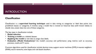
Classification is a supervised learning technique used in data mining to categorize or label data points into
predefined classes or categories. It involves using a model that is trained on historical data (with known labels) to
classify new, unseen data into one of these categories.
The key steps in classification include:
• Model selection
• Training a model on a labeled dataset.
• Applying the model to new data to assign class labels.
• Evaluation (Model Evaluation)of the model's accuracy and performance using metrics such as accuracy,
precision, recall, and F1 score.
Common algorithms used for classification include decision trees, support vector machines (SVM), k-nearest neighbors
(KNN), neural networks, naïve bayes and rule based classifiers.

3. INTRODUCTION
Prediction
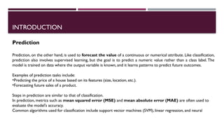
Prediction, on the other hand, is used to forecast the value of a continuous or numerical attribute. Like classification,
prediction also involves supervised learning, but the goal is to predict a numeric value rather than a class label. The
model is trained on data where the output variable is known, and it learns patterns to predict future outcomes.
Examples of prediction tasks include:
•Predicting the price of a house based on its features (size, location, etc.).
•Forecasting future sales of a product.
Steps in prediction are similar to that of classification.
In prediction, metrics such as mean squared error (MSE) and mean absolute error (MAE) are often used to
evaluate the model's accuracy.
Common algorithms used for classification include support vector machines (SVM), linear regression, and neural

4. INTRODUCTION
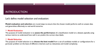
Let’s define model selection and evaluation:
Model evaluation and selection are crucial steps to ensure that the chosen model performs well on unseen data
and generalizes effectively to real-world scenarios.
 Model Evaluation
The purpose of model evaluation is to assess the performance of a classification model on a dataset, typically using
various metrics to understand how well it can predict the correct class labels.
 Model Selection
The purpose of model selection is to choose the best model from a set of candidate models or configurations for a
particular problem on the basis of different criterions such as robustness and model complexity.

5. CLASSIFICATION
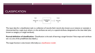
The input data for a classification task is a collection of records. Each record, also known as an instance or example, is
characterized by a tuple (x,y), where x is the attribute set and y is a special attribute, designated as the class label (also
known as category or target attribute).
Formal definition of classification: Classification is the task of learning a target function f that maps each attribute
set x to one of the predefined class Iabels y.
The target function is also known informally as a classification model.

6. GENERAL APPROACHTO SOLVING A CLASSIFICATION PROBLEM

7. GENERAL APPROACHTO SOLVING A CLASSIFICATION PROBLEM
• A classification technique (or classifier) is a systematic approach to building classification models from an input data
set. Each technique employs a learning algorithm to identify a model that best fits the relationship between the
attribute set and class label of the input data.The model generated by a learning algorithm should both fit the input
data well and correctly predict the class labels of records it has never seen before.Therefore, a key objective of the
learning algorithm is to build models with good generalization capability; i.e., models that accurately predict the class
labels of previously unknown records.
• Approach:
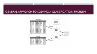
 First step is to partition the dataset into train set and test set.Various techniques to partition the dataset are :
1. Holdout method
2. K-fold cross validation
3. Leave one out
Class labels for the records in the train set are known.
 Next, the classifier is built from the training set.This is known as learning or training phase. Model learns the
relationship between the attributes and the class labels of the dataset

8. GENERAL APPROACHTO SOLVING A CLASSIFICATION PROBLEM
 Then, the classifier is applied to the test set (records for which class labels are unknown) to evaluate its
performance.
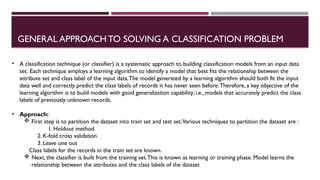
 Evaluation of the performance of a classification model is based on the counts of test records correctly and
incorrectly predicted by the model.These counts are tabulated in a table known as a confusion matrix.
• TabIe 4.2 depicts the confusion matrix for a binary classification problem. Each entry fij in this table
denotes the number of records from class i predicted to be of class j. For instance, f01 is the number of
records from class 0 incorrectly predicted as class 1. Based on the entries in the confusion matrix, the total
number of correct predictions made by the model is (f11 + f00) and the total number of incorrect
predictions is (f10 + f01).

9. GENERAL APPROACHTO SOLVING A CLASSIFICATION PROBLEM
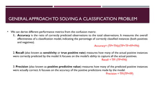
• We can derive different performance metrics from the confusion matric:
1. Accuracy is the ratio of correctly predicted observations to the total observations. It measures the overall
effectiveness of a classification model, indicating the percentage of correctly classified instances (both positives
and negatives).
Accuracy= (TP+TN)/(TP+TF+FP+FN)
2. Recall (also known as sensitivity or true positive rate) measures how many of the actual positive instances
were correctly predicted by the model. It focuses on the model's ability to capture all the actual positives.
Recall = TP/ (TP+FN)
3. Precision (also known as positive predictive value) measures how many of the predicted positive instances
were actually correct. It focuses on the accuracy of the positive predictions made by the model.
Precision = TP/(TP+FP)

10. GENERAL APPROACHTO SOLVING A CLASSIFICATION PROBLEM
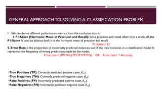
• We can derive different performance metrics from the confusion matric:
4. F1-Score (Harmonic Mean of Precision and Recall): Since precision and recall often have a trade-off, the
F1-Score is used to balance both. It is the harmonic mean of precision and recall:
F1-Score = 2×
5. Error Rate is the proportion of incorrectly predicted instances out of the total instances in a classification model. It
represents the frequency of wrong predictions made by the model.
Error rate = (FP+FN)/(TP+TF+FP+FN) OR Error rate= 1-Accuracy
•True Positives (TP): Correctly predicted positive cases. (f11)
•True Negatives (TN): Correctly predicted negative cases. (f00)
•False Positives (FP): Incorrectly predicted positive cases (f01).
•False Negatives (FN): Incorrectly predicted negative cases (f10).

11.  Most classification algorithms seek models that attain the highest accuracy, or equivalently, the lowest error rate
when applied to the test set.
 Various techniques to increase the accuracy of the model:
 Adding a penalty to the loss function to prevent overfitting.
 Addressing class imbalance issues by techniques such as oversampling the minority class, undersampling the
majority class, or using class weights.
 Using techniques like k-fold cross-validation to ensure that the model generalizes well to unseen data by
training and validating it on different subsets of the data.
GENERAL APPROACHTO SOLVING A CLASSIFICATION PROBLEM

12. CHALLENGES/ ISSUES IN CLASSIFICATION
Classification and prediction face several challenges that can affect the accuracy, reliability, and applicability of models:
1. Imbalanced dataset: In many classification tasks, the data is imbalanced, meaning one class significantly
outnumbers the other(s). This leads to misclassification because classifiers tend to focus on the majority class.
2. Overfitting and underfitting: When the model learns not only the patterns but also the noise in the training
data, it performs well on training data but poorly on new, unseen data.This is the case of overfitting. In underfitting,
the model is too simple to capture the underlying patterns in the data, leading to poor performance on both
training and test data. Balancing the model’s complexity to avoid both overfitting and underfitting is crucial.
3. High Dimensionality: When the dataset has a large number of features (high dimensionality), it becomes difficult
to model the data efficiently.The "curse of dimensionality" refers to the fact that the volume of data increases
exponentially with the number of features, making it hard to generalize.
4. Bias-Variance tradeoff: A model with high bias may be too simplistic (underfitting), while a model with high
variance may overfit the training data. Achieving a balance between bias and variance is difficult, as reducing one
often increases the other.

13. IMBALANCED DATASET
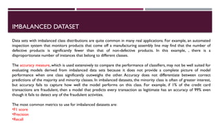
Data sets with imbalanced class distributions are quite common in many real applications. For example, an automated
inspection system that monitors products that come off a manufacturing assembly line may find that the number of
defective products is significantly fewer than that of non-defective products. In this example, , there is a
disproportionate number of instances that belong to different classes.
The accuracy measure, which is used extensively to compare the performance of classifiers, may not be well suited for
evaluating models derived from imbalanced data sets because it does not provide a complete picture of model
performance when one class significantly outweighs the other. Accuracy does not differentiate between correct
predictions of the majority and minority classes. In imbalanced datasets, the minority class is often of greater interest,
but accuracy fails to capture how well the model performs on this class. For example, if 1% of the credit card
transactions are fraudulent, then a model that predicts every transaction as legitimate has an accuracy of 99% even
though it fails to detect any of the fraudulent activities.
The most common metrics to use for imbalanced datasets are:
•F1 score
•Precision
•Recall

14. IMBALANCED DATASET
For a highly imbalanced dataset, well-suited algorithms:
• SupportVector Machines : SVM can be adapted for imbalanced datasets using class weighting.
• Naive Bayes: Naive Bayes can work surprisingly well with imbalanced datasets, especially when the assumptions of
conditional independence hold. Since it relies on probabilities, it can still perform adequately even with skewed class
distributions.

15. CLASSIFICATION ALGORITHMS
We will discuss the following algorithms:
1. Decision tree
2. Naïve Bayes classifier
3. Rule based classifier
4. SupportVector Machine
5. Neural Networks