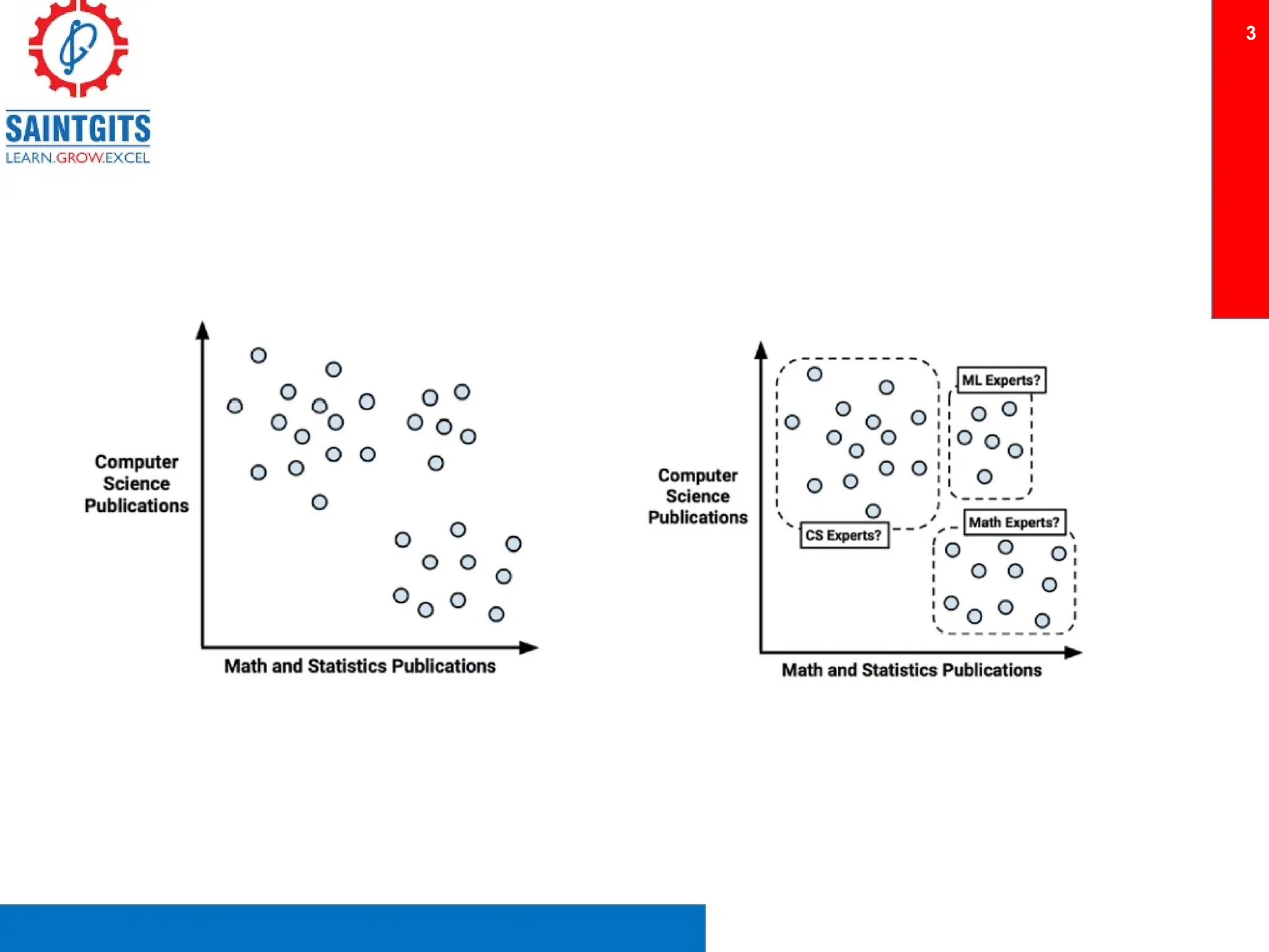
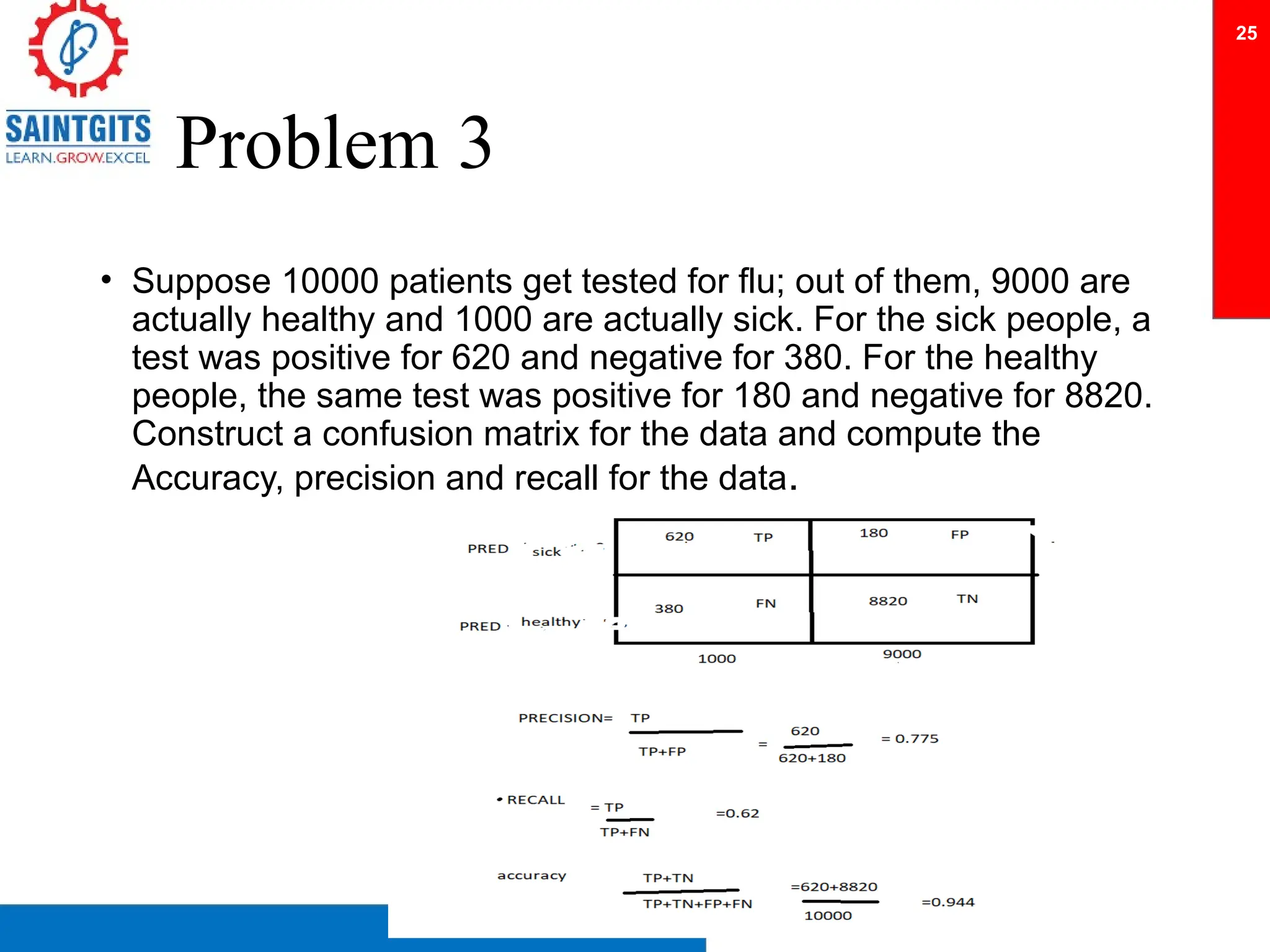
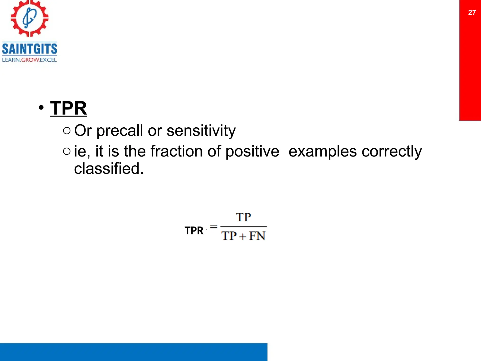
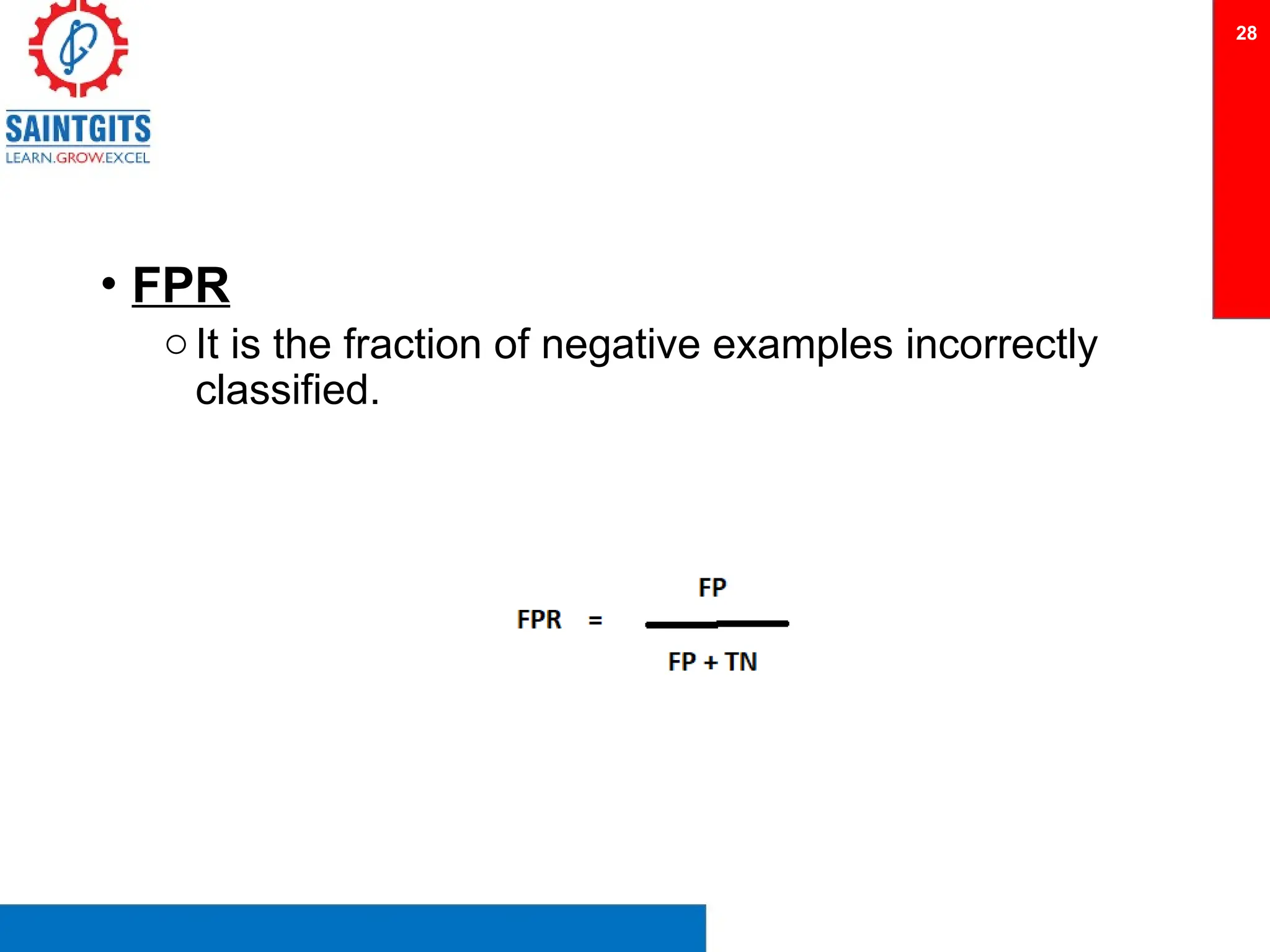
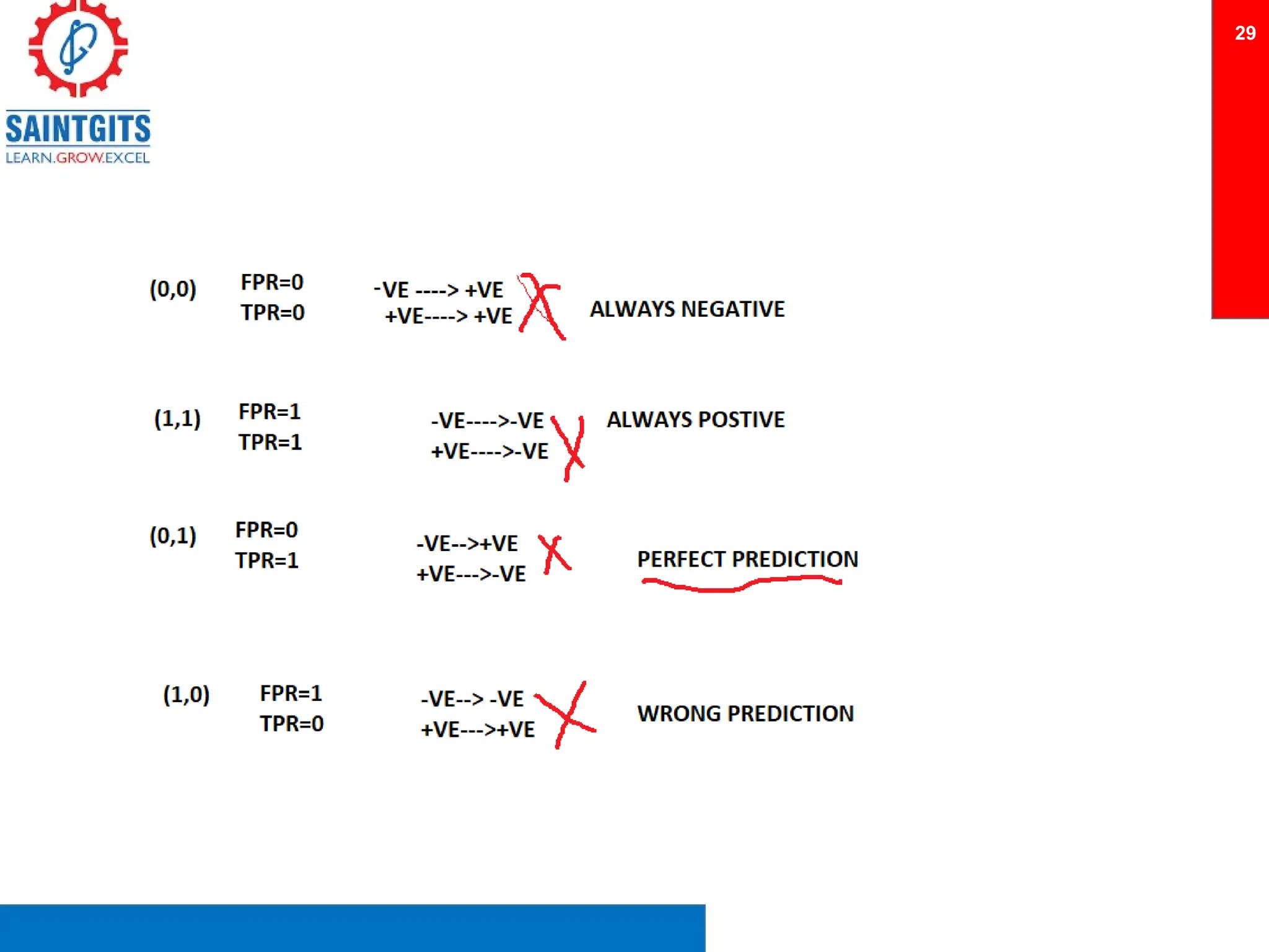
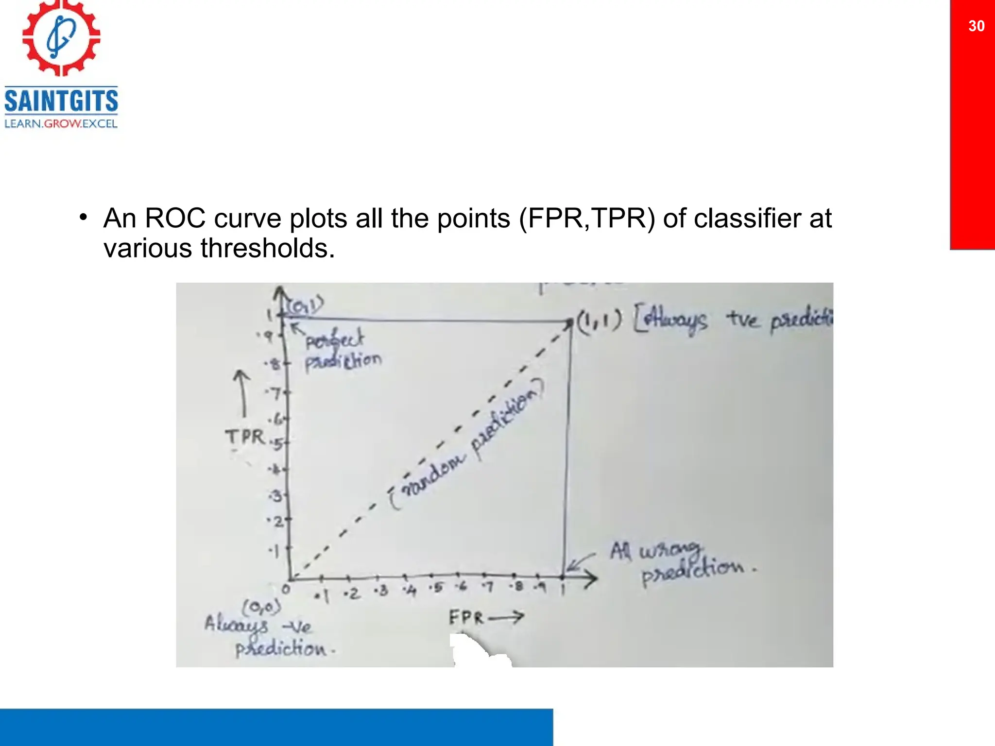
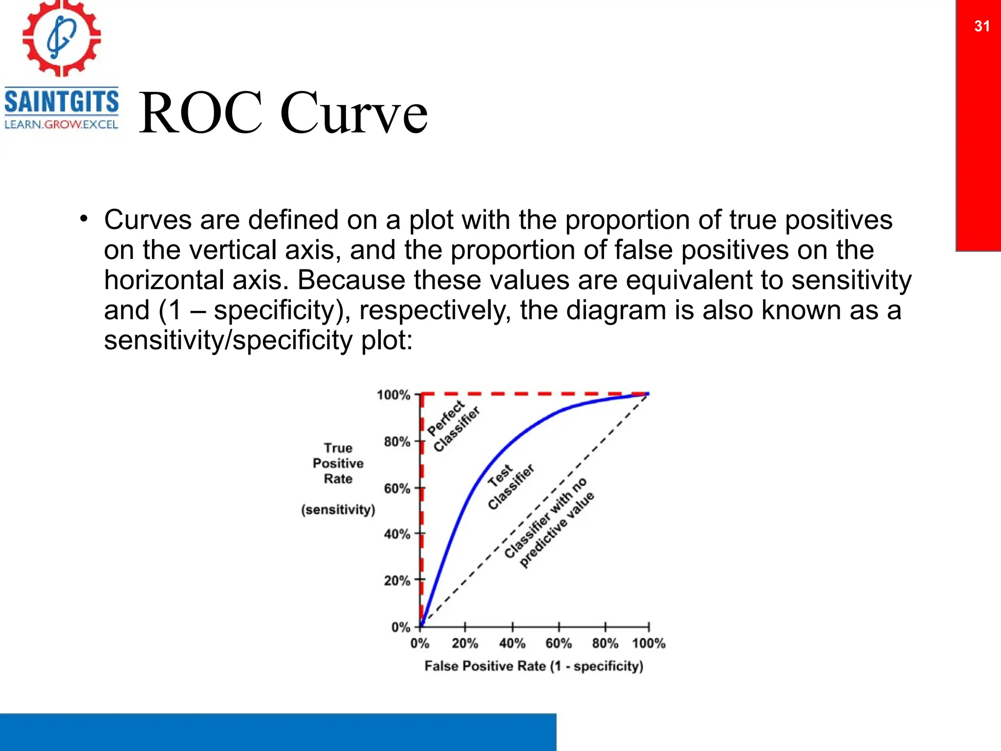
Clustering is an unsupervised learning technique that groups similar items together, and is applied in various domains like customer segmentation and anomaly detection. Key clustering algorithms include k-means and hierarchical clustering, with k-means focused on minimizing intra-cluster variance and maximizing inter-cluster differences. Additionally, model performance assessment involves metrics like precision, recall, accuracy, and ROC curves, with methods like cross-validation and ensemble learning employed to enhance predictive modeling.

1. Clustering
• Clustering or cluster analysis is an unsupervised learning
algorithm.
• it is automatically divides the data into clusters, or groups of
similar items.
• Clustering is guided by the principle that items inside a cluster
should be very similar to each other, but very different from those
outside.
1

2. The resulting clusters can then be used for action. For instance, you might
find clustering methods employed in the following applications:
• Segmenting customers into groups with similar demographics or buying
patterns for targeted marketing campaigns
• Detecting anomalous behaviour, such as unauthorized network intrusions,
by identifying patterns of use falling outside the known clusters
• Simplifying extremely large datasets by grouping features with similar
values into a smaller number of homogeneous categories
2

3. 3

4. Various algorithms are:
•K-Mean clustering
•Hierarchical Clustering
•Density-based Clustering
•Expectation–maximization clustering
4

5. The k-means clustering algorithm
• The k-means algorithm assigns each of the n examples to one of
the k clusters, where k is a number that has been determined
ahead of time
• The goal is to minimize the differences within each cluster and
maximize the differences between the clusters.
5

6. Algorithm
Step1 : Randomly select k cluster centers ,V1,V2,V3….
Step2 : Calculate the distance between each data point and cluster
centres Vi
Step 3: Assign each data point Aj to the cluster center Vi for which
the distance ||Aj-Vi|| is minimum.
Step 4: Recalculate each cluster center by taking the average of
cluster’s data points
Step 5 : Repeat from step2 to step 5 until the recalculated cluster
centers are same as previous or no re assignment of data
points happened
6

7. Distance between data points
• We assume that each data point is a n – dimensional vecor
• The distance between two data points
X=(x1,x2,x3….,xn)
And
Y=(y1,y2,y3…,yn)
the formula for Euclidean distance between example x and example
y is:
7

8. Choosing the appropriate number of
clusters
• The elbow method is used to determine the optimal number of
clusters in k-means clustering.
• A technique known as the elbow method attempts to gauge how
the homogeneity or heterogeneity within the clusters changes for
various values of k
• As illustrated in the following diagrams, the homogeneity within
clusters is expected to increase as additional clusters are added;
similarly, heterogeneity will also continue to decrease with more
clusters.
• the goal is not to maximize homogeneity or minimize
• heterogeneity, but rather to find k so that there are diminishing
returns beyond that point. This value of k is known as the elbow
point
8

9. 9

10. 10

11. Confusion matrices
• A confusion matrix is a table that categorizes predictions according to
whether they match the actual value. One of the table's dimensions
indicates the possible categories of predicted values, while the other
dimension indicates the same for actual values. Although we have only
seen 2 x 2 confusion matrices so far, a matrix can be created for models
that predict any number of class values. The following figure depicts the
familiar confusion matrix for a two-class binary model as well as the 3 x 3
confusion matrix for a three-class model
11

12. 12

13. • The most common performance measures consider the model's
ability to discern one class versus all others. The class of interest
is known as the positive class, while all others are known as
negative
• The relationship between the positive class and negative class
predictions can be depicted as a 2 x 2 confusion matrix that
tabulates whether predictions fall into one of the four categories
13

14. The relationship between the positive class and negative class predictions
can be depicted as a 2 x 2 confusion matrix that tabulates whether
predictions fall into one of the four categories:
• True Positive (TP): Correctly classified as the class of interest
• True Negative (TN): Correctly classified as not the class of interest
• False Positive (FP): Incorrectly classified as the class of interest
• False Negative (FN): Incorrectly classified as not the class of interest
14

15. Precision and recall
• It is the ratio between true positives and all the
predicted positives.
• Precision is a measure of how many samples
are correctly identified as +ve out of all the
samples which are predicted as +ve.
15

16. `
• Recall : it is the ratio between true positives
and all the actual positives.
• Recall is a measure of how many samples are
correctly identified as +ve out of all the
samples which are actually +ve.
16

17. 17

18. Other Measures
Accuracy
With the 2 x 2 confusion matrix, we can formalize our definition of
prediction accuracy (sometimes called the success rate) as:
In this formula, the terms TP, TN, FP, and FN refer to the number of
times the model's predictions fell into each of these categories.
Therefore, the accuracy is the proportion that represents the
number of true positives and true negatives divided by the total
number of predictions.
18

19. • error rate
The error rate, or the proportion of incorrectly classified
examples, is specified as:
Notice that the error rate can be calculated as one minus the
accuracy. Intuitively, this makes sense; a model that is correct 95
percent of the time is incorrect 5 percent of the time
19

20. • Sensitivity
The sensitivity of a model (also called the true positive rate), measures the
proportion of positive examples that were correctly classified. Therefore,
as shown in the following formula, it is calculated as the number of true
positives divided by the total number of positives in the data—those
correctly classified (the true positives), as well as those incorrectly
classified (the false negatives).
20

21. • specificity
The specificity of a model (also called the true negative rate), measures the
proportion of negative examples that were correctly classified. As with
sensitivity, this is computed as the number of true negatives divided by
the total number of negatives—the true negatives plus the false positives.
21

22. • The F-measure
A measure of model performance that combines precision and recall
into a single number is known as the F-measure (also sometimes
called the F1 score or the F-score). The F-measure combines
precision and recall using the harmonic mean. The harmonic
mean is used rather than the more common arithmetic mean
since both precision and recall are expressed as proportions
between zero and one. The following is the formula for F-
measure:
22

23. Problem 1
Suppose a computer program for recognizing dogs in a
photographs identifies 8 dogs in a picture containing 12 dogs and
some cats. Of the 8 dogs identified , 5 actually are dogs while rest of
them are cats. Compute the precision and recall for the computer.
23

24. Problem 2
• Let there be 10 balls (6 white and 4 red balls) in a box and let it be
required to pick up the red balls from them. Suppose we pick up 7
balls as the red balls, of which only 2 are actually red balls.what
are the values of precision and recall in picking red ball?
24

25. Problem 3
• Suppose 10000 patients get tested for flu; out of them, 9000 are
actually healthy and 1000 are actually sick. For the sick people, a
test was positive for 620 and negative for 380. For the healthy
people, the same test was positive for 180 and negative for 8820.
Construct a confusion matrix for the data and compute the
Accuracy, precision and recall for the data.
25

26. ROC curves
• ROC curve (Receiver Operating Characteristic)
• An ROC curve is a graph showing the performance of a classifier
at all classification thresholds.
• The curve plots two parameters
• True positive rate(TPR)
• False positive rate(FPR)
26

27. • TPR
oOr precall or sensitivity
oie, it is the fraction of positive examples correctly
classified.
27
TPR

28. • FPR
oIt is the fraction of negative examples incorrectly
classified.
28

29. 29

30. • An ROC curve plots all the points (FPR,TPR) of classifier at
various thresholds.
30

31. ROC Curve
• Curves are defined on a plot with the proportion of true positives
on the vertical axis, and the proportion of false positives on the
horizontal axis. Because these values are equivalent to sensitivity
and (1 – specificity), respectively, the diagram is also known as a
sensitivity/specificity plot:
31

32. • The closer the curve is to the perfect classifier, the better it is at
identifying positive values. This can be measured using a statistic
known as the area under the ROC curve (abbreviated AUC).
32

33. Cross validation
• To test the performance of a classifier , we
need to have a number of training /validation
set pairs.
33

34. • Cross validation methods are used for generating multiple training
validation sets from a given dataset.
• Cross validation is technique to evaluate predictive models by
partitioning the original sample into a training set to train the
model and test set to evaluate it.
• Different methods are:
1. Hold out method
2. K-fold cross validation
3. Leave-one-out cross validation
4. Bootstrapping
34

35. Holdout method
• The dataset is separated into two sets, called the training set and
the testing set
• The algorithm fits a function using training set only. Then the
function is used to predict the output values for the data in the
testing set.
35

36. • As shown in the following diagram, the training dataset is used to
generate the model, which is then applied to the test dataset to
generate predictions for evaluation. Typically, about one-third of
the data is held out for testing and two-thirds used for training, but
this proportion can vary depending on the amount of data
available. To ensure that the training and test data do not have
systematic differences, examples are randomly divided into the
two groups.
36

37. • One problem with holdout sampling is that each partition may
have a larger or smaller proportion of some classes. In certain
cases, particularly those in which a class is a very small
proportion of the dataset, this can lead a class to be omitted from
the training dataset—a significant problem, because the model
cannot then learn this class.
• In order to reduce the chance that this will occur, a technique
called stratified random sampling can be used. Although, on
average, a random sample will contain roughly the same
proportion of class values as the full dataset, stratified random
sampling ensures that the generated random partitions have
approximately the same proportion of each class as the full
dataset.
37

38. • Advantages
• Simple and easy to run
• Lower computational cost as it only needs to be
run once.
• Disadvantages
• Only work on large dataset
• Higher variance given the smaller size of the data.
38

39. K-Fold cross validation
• The dataset X is divided randomly into K equal-sized parts , Xi,
i=1,2…,k.
39

40. 40

41. 41

42. • To generate each pair, we keep one of the K parts out as the
validation set Vi, and combine the remaining K-1 parts to form the
training Ti.
• Doing this K times, we get K pairs (Vi, Ti).
Problems with this approach
• To keep the training set large we allow validation sets to be small
• Every two training sets share k-2 parts.
42

43. • K is typically 10 or 30 .As K increases the percentage of training
instances increases and we get more robust estimators, but the
validation set becomes smaller. Also the cost of training the
classifier increases as k increases.
43

44. Example
Consider a dataset containing 30 samples and let K=5.then we
divide dataset int 5 folds, each fold containing 6 samples.
44

45. Bootstrapping
• Also known as bootstrap sampling,bootstarp, or random sampling
with replacement.
• Bootstrapping is the process of computing performance measure
using several randomly selected training and test datasets which
are selected through a process of sampling with replacement.
• The bootstrap procedure will create one or more new training
datasets some of which are repeated
• The corresponding test datasets are then constructed from the set
of examples that were not selected of the respective training
datasets.
45

46. Ensemble learners
• No single learning algorithm is a most accurate
learners.
• Try many learners and choose the one that performs
the best on the validation set.
• Combine multiple learning algorithms or same
algorithm with different hyperparameter as classifier
46

47. • Reason to combine many learners together
• Single learner may not produce accurate results.
47

48. Base Learners
• Individual algorithms in the collection of machine learning
algorithms are called base learners.
• When we generate multiple base learners it should be
reasonability accurate.
48

49. What is an ensemble learning?
• Ensemble learning is a machine learning techniques where
multiple models are combined to solve the same problem.
• As the name suggests , ensemble learning utilizes the advantages
of multiple base models(usually called “ weak learners”) to
compensate each models weaknesses.
• The main principle behind ensemble learning is to group weak
learners together to form one strong learner(or “ensemble model”)
that achieves better performance than any individual weak
learner.
49

50. Why the weak learners are
called weak?
• In ensemble learning theory , we call “weak learner” the models
that perform not so well by themselves either because they have a
high bias or because they have a high variance.
• The ensemble learning models can be categorized into two types
based on the choice of weak learners: homogenous and
heterogeneous.
50

51. • In homogeneous ensemble model , a single base learning
algorithm is used.
• For example, all weak learns are based on decision (DT)
algorithm.
51

52. • In heterogenous ensemble model, different base
learning algorithms are used.
• For example , the weak learns are based on decision
tree, support vector machines and k-nearest
neighbours algorithms.
52

53. Combining the weak learners
• However, note that the choice of weak learners should be
coherent with the way we combine these models.
• For examples if we choose the base models with high variance
and low bias, then the combination method should aim to reduce
the variance.
53

54. • There are three popular combination methods
1.Bagging(considers homogenous weak learners, focuses on
reducing the variance)
2.Boosting(considers homogenous weak learners, focuses on
reducing the bias)
3.Stacking(considers heterogenous weak learners)
54

55. Understanding ensembles
• Suppose you were a contestant on a television trivial show that
allowed you to choose a panel of five friends to assist you with
answering the final question for the million-dollar prize. Most
people would try to stack the panel with a diverse set of subject-
matter experts. For instance, a panel containing professors of
literature, science, history, and art, along with a current pop-
culture expert would be a safely well-rounded group. Given their
breadth of knowledge, it would be unlikely to find a question that
stumps the panel.
• The meta-learning approach that utilizes a similar principle of
creating a varied team of experts is known as an ensemble. All
ensemble methods are based on the idea that by combining
multiple weaker learners, a stronger learner is created
55

56. it can be helpful to imagine the ensemble in terms of the
process diagram as follows
56

57. • First, input training data is used to build a number of models. The allocation function
dictates whether each model receives the full training dataset or merely a sample.
• Since the ideal ensemble includes a diverse set of models, the allocation function could
increase diversity by artificially varying the input data to train a variety of learners.
• On the other hand, if the ensemble already includes a diverse set of algorithms—such
as a neural network, a decision tree, and a kNN classifier—then the allocation function
might pass on the data relatively unchanged.
• After the models are constructed, they can be used to generate a set of predictions,
which must be managed in some way. The combination function governs how
disagreements among the predictions are reconciled.
• For example, the ensemble might use a majority vote to determine the final prediction,
or it could use a more complex strategy such as weighting each model's votes based
on its prior performance.
• Some ensembles even utilize another model to learn a combination function from
various combinations of predictions.
• This process of using the predictions of several models to train a final arbiter model is
known as stacking
57

58. • One of the benefits of using ensembles is that they may allow you
to spend less time in pursuit of a single best model. Instead, you
can train a number of reasonably strong candidates and combine
them.
58

59. Ensembles also offer a number of performance
advantages over single models:
• Better generalizability to future problems
• Improved performance on massive or miniscule datasets:
• The ability to synthesize of data from distinct domains:
• A more nuanced understaSnding of difficult learning tasks:
59

60. Bagging
• The bagging method(stands for bootstrap aggregating”) aims to produce
an ensemble model that has less variance(i.e., more robust) than its
components.
• It first learns several homogenous weak learners with high
variance(independently from each other) and then combines them by
using some “ averaging” process.
• One important question is how to obtain so much data to train the weak
learners?
• The solution is to use bootstrapping!
60

61. bootstrapping
• Imagine that we are given dataset of patients
MRI records consisting of 5 samples.
61

62. 62

63. 63

64. • This process is repeated until we create a
bootstrapped dataset for every weak learner.
64

65. 65

66. 66

67. 67

68. 68

69. To sum up, the bagging algorithm can be described as follows.
1.Create many random subsets of the initial dataset by using the
bootstrapping.
2.Train a machine learning model on each subset.
3.Average the predictions from all the models.
69

70. • One of the popular bagging examples is the random forest
algorithm.
• In random forest , multiple deep decision trees with high variance
are trained on bootstrapped datasets and combined to produce an
ensemble model with lower variance.
70

71. Boosting
• Boosting methods follow the same principle as bagging: multiple
homogeneous weak learners are combined to obtain a strong learner that
performs better than any individual weak learner.
71

72. • However, unlike the bagging that mainly aims at
reducing the variance , the boosting aims at reducing
the bias.
72

73. • Consequently , the base models that are often considered for
boosting are models with low variance and high bias.
73

74. • While in bagging the base models are trained independently from
each other, in boosting the base models are trained
sequentially(or iteratively).
74

75. • Another important feature of boosting is that each model in the
sequence is trained giving more importance to samples in the
dataset that were badly handled by the previous models in the
sequence.
• Consequently, each new model focuses its efforts on the most
difficult samples.
75

76. 76

77. 77

78. 78

79. 79

80. • Step1:
• The base learners takes all the distributions and assign equal weights or
attention to each observation.
• Step2:
• If there is any prediction error caused by first base learning algorithm, then we
pay higher attention weights to observations having prediction error . Then
we apply the next base learning algorithm.
• Step3:
• Iterate step2 till the limit of base learning algorithm and reached or higher
accuracy is achieved.
80

81. 81

82. • A boosting algorithm called AdaBoost, or adaptive boosting, was
proposed in 1997. The algorithm is based on the idea of generating
weak leaners that iteratively learn a larger portion of the difficult-to-
classify examples in the training data by paying more attention (that
is, giving more weight) to often misclassified examples.
• Beginning from an unweighted dataset, the first classifier attempts
to model the outcome. Examples that the classifier predicted
correctly will be less likely to appear in the training dataset for the
following classifier, and conversely, the difficult-to-classify examples
will appear more frequently. As additional rounds of weak learners
are added, they are trained on data with successively more difficult
examples. The process continues until the desired overall error rate
is reached or performance no longer improves. At that point, each
classifier's vote is weighted according to its accuracy on the training
data on which it was built
82

83. • The AdaBoost.M1 algorithm provides an alternative tree-based
implementation of AdaBoost for classification.
• A tree with just one node and two leaf is called stump.
• Stumps are technically weak learners
• In random forest each tree has equal vote on the final
classification
• In contrast, in a forest of stumps made with Adaboost, some
stumps get more say in the final classification than others
83

84. Stacking
84

85. 85

86. 86

87. 87

88. 88

89. • Instead of 2-fold , we can also use k-fold cross-training(similar to
k-fold cross-validation) where all samples are used to train both
the weak learners and the meta-model.
• In k-fold cross-training, k-1 folds are used to train the weak
learners whereas the remaining fold is used to train the meta-
model(repeated iteratively).
89

90. 90

91. Random forests
• Another ensemble-based method called random forests (or
decision tree forests) focus only on ensembles of decision trees.
This method was championed by Leo Breiman and Adele Cutler,
and combines the base principles of bagging with random feature
selection to add additional diversity to the decision tree models.
After the ensemble of trees (the forest) is generated, the model
uses a vote to combine the trees' predictions.
• Random forests combine versatility and power into a single
machine learning approach. Because the ensemble uses only a
small, random portion of the full feature set, random forests can
handle extremely large datasets, where the so-called "curse of
dimensionality" might cause other models to fail. At the same time,
its error rates for most learning tasks are on par with nearly any
other method.
91

92. 92

93. 93

94. 94