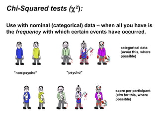
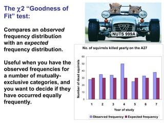
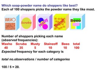
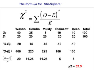
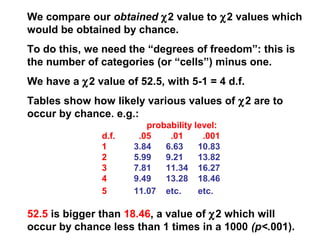
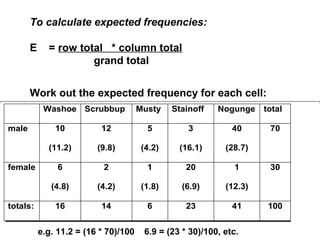
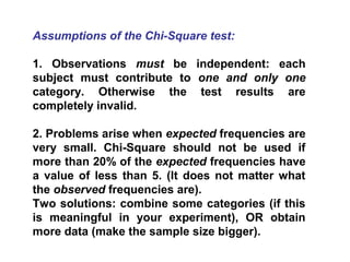
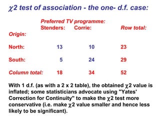
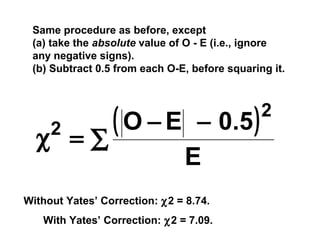
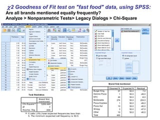
- Chi-squared (χ2) tests are used to analyze categorical data by comparing observed frequencies to expected frequencies. - The document provides examples of using the χ2 test to test if frequency distributions match expected distributions (goodness of fit test) and to test for associations between two categorical variables. - Key assumptions and considerations for χ2 tests are that observations must be independent and expected frequencies should not be too small.

1. Chi-Squared tests (χ2
):

2. Chi-Squared tests (χ2
):
Use with nominal (categorical) data – when all you have is
the frequency with which certain events have occurred.
score per participant
(aim for this, where
possible)
categorical data
(avoid this, where
possible)
"psycho""non-psycho"

3. The χ2 “Goodness of
Fit” test:
Compares an observed
frequency distribution
with an expected
frequency distribution.
Useful when you have the
observed frequencies for
a number of mutually-
exclusive categories, and
you want to decide if they
have occurred equally
frequently.
No. of squirrels killed yearly on the A27
0
10
20
30
40
50
60
1 2 3 4 5 6 7
Year of study
Numberofdeadsquirrels
Observed frequency Expected frequency

4. Which soap-powder name do shoppers like best?
Each of 100 shoppers picks the powder name they like most.
Number of shoppers picking each name
(observed frequencies):
Washo Scruba Musty Stainzoff Beeo total
40 35 5 10 10 100
Expected frequency for each category is
total no.observations / number of categories
100 / 5 = 20.

5. ( )
∑
−
=
E
EO
22
χ
The formula for Chi-Square:
( )
E
EO −
2
Washo Scruba Musty Stainzoff Beeo total
O: 40 35 5 10 10 100
E: 20 20 20 20 20 100
(O-E): 20 15 -15 -10 -10
(O-E) 2
400 225 225 100 100
20 11.25 11.25 5 5
χ2 = 52.5

6. Chi-squared is the sum of the squared
differences between each observed frequency
and its associated expected frequency.
The bigger the value of χ2, the greater the
difference between observed and expected
frequencies.
But how big does χ2 have to be, to be regarded
as “big”? Is 52.5 “big”?

7. We compare our obtained χ2 value to χ2 values which
would be obtained by chance.
To do this, we need the “degrees of freedom”: this is
the number of categories (or “cells”) minus one.
We have a χ2 value of 52.5, with 5-1 = 4 d.f.
Tables show how likely various values of χ2 are to
occur by chance. e.g.:
probability level:
d.f. .05 .01 .001
1 3.84 6.63 10.83
2 5.99 9.21 13.82
3 7.81 11.34 16.27
4 9.49 13.28 18.46
5 11.07 etc. etc.
52.5 is bigger than 18.46, a value of χ2 which will
occur by chance less than 1 times in a 1000 (p<.001).

8. The sampling distribution of chi-square:
Frequency with which χ2 values occur purely by
chance:
With 4 d.f., χ2 values of 9.49 or more
are likely to occur by chance on less
than .05 of occasions.

9. Our obtained χ2 = 52.5, with 4 d.f., p < .001.
A χ2 value this large is highly unlikely to have
arisen by chance.
It appears that the distribution of shoppers’
choices across soap-powder names is not
random. Some names get picked more than we
would expect by chance and some get picked
less.

10. The χ2 test of association between two
independent variables:
Another common use of χ2 is to determine whether
there is an association between two independent
variables.
Is there an association between gender (male or
female: IV A) and soap powder (Washo, Musty, etc.:
IV B)?

11. This gives a 2 x 5 contingency table.
Data for a random sample of 100 shoppers, 70 men and
30 women:
Washoe Scrubbup Musty Stainoff Nogunge total
male 10 12 5 3 40 70
female 6 2 1 20 1 30
totals: 16 14 6 23 41 100

12. To calculate expected frequencies:
E = row total * column total
grand total
Work out the expected frequency for each cell:
Washoe Scrubbup Musty Stainoff Nogunge total
male 10
(11.2)
12
(9.8)
5
(4.2)
3
(16.1)
40
(28.7)
70
female 6
(4.8)
2
(4.2)
1
(1.8)
20
(6.9)
1
(12.3)
30
totals: 16 14 6 23 41 100
e.g. 11.2 = (16 * 70)/100 6.9 = (23 * 30)/100, etc.

13. Using exactly the same formula as before, we get χ2
= 52.94.
d.f. = (number of rows - 1) * (number of columns - 1).
We have two rows and five columns,
so d.f. = (2-1) * (5-1) = 4 d.f.
Use the same table to assess the chances of
obtaining a Chi-Squared value as large as this by
chance; again p< .001.
Conclusion: our observed frequencies are
significantly different from the frequencies we would
expect to obtain if there were no association
between the two variables: i.e. the pattern of name
preferences is different for men and women.

14. Chi-Square test merely tells you that there is some
relationship (an association) between the two
variables in question: it does not tell you anything
about the causal relationship between the two
variables.
Here, it is reasonable to assume that gender
causes people to pick different soap powder
names; it's unlikely that soap powder names
cause people to be male or female.
However, in principle the direction of causality
could equally well go in either direction.

15. Assumptions of the Chi-Square test:
1. Observations must be independent: each
subject must contribute to one and only one
category. Otherwise the test results are
completely invalid.
2. Problems arise when expected frequencies are
very small. Chi-Square should not be used if
more than 20% of the expected frequencies have
a value of less than 5. (It does not matter what
the observed frequencies are).
Two solutions: combine some categories (if this
is meaningful in your experiment), OR obtain
more data (make the sample size bigger).

16. χ2 test of association - the one- d.f. case:
Preferred TV programme:
Stenders: Corrie: Row total:
Origin:
North: 13 10 23
South: 5 24 29
Column total: 18 34 52
With 1 d.f. (as with a 2 x 2 table), the obtained χ2 value is
inflated; some statisticians advocate using "Yates'
Correction for Continuity" to make the χ2 test more
conservative (i.e. make χ2 value smaller and hence less
likely to be significant).

17. Same procedure as before, except
(a) take the absolute value of O - E (i.e., ignore
any negative signs).
(b) Subtract 0.5 from each O-E, before squaring it.
( )
∑
−−
=χ
E
0.5EO
2
2
Without Yates’ Correction: χ2 = 8.74.
With Yates’ Correction: χ2 = 7.09.

18. Why you should avoid using Chi-Square if you can:
Design studies so that you can avoid using Chi-
Square!
Frequency data give little information about
participants' performance: all you have is
knowledge about which category someone is in, a
very crude measure.
It's much more informative to obtain one or more
scores per participant; scores give you more
information about performance than categorical
data (and can be used with better statistical tests).
e.g. IQ: which is better - to know participants are
“bright” or “dim”, or have their actual IQ scores?

19. χ2 Goodness of Fit test on "fast food" data, using SPSS:
Are all brands mentioned equally frequently?
Analyze > Nonparametric Tests> Legacy Dialogs > Chi-Square
Brand first mentioned
57 50.0 7.0
1 50.0 -49.0
44 50.0 -6.0
274 50.0 224.0
1 50.0 -49.0
10 50.0 -40.0
3 50.0 -47.0
10 50.0 -40.0
400
Burger King
Domino Pizza
KFC
McDonalds
Pizza Express
Pizza Hut
Wimpy
Other
Total
Observed N Expected N Residual
Test Statistics
1209.440
7
.000
Chi-Square a
df
Asymp. Sig.
Brand first
mentioned
0 cells (.0%) have expected frequencies less than
5. The minimum expected cell frequency is 50.0.
a.

20. χ2 test of association on "fast food" data, using SPSS:
Is there an association between gender and brand first mentioned?
Analyze > Descriptive Statistics > Crosstabs...

21. χ2 test of association on "fast food" data (continued):
Is there an association between gender and brand first mentioned?
Case Processing Summary
375 100.0% 0 .0% 375 100.0%
Sex * Brand
first mentioned
N Percent N Percent N Percent
Valid Missing Total
Cases
Sex * Brand first mentioned Crosstabulation
30 21 135 186
28.3 21.8 135.9 186.0
27 23 139 189
28.7 22.2 138.1 189.0
57 44 274 375
57.0 44.0 274.0 375.0
Count
Expected Count
Count
Expected Count
Count
Expected Count
Male
Female
Sex
Total
Burger King KFC McDonalds
Brand first mentioned
Total
Chi-Square Tests
.283a 2 .868
.283 2 .868
.135 1 .714
375
Pearson Chi-Square
Likelihood Ratio
Linear-by-Linear
Association
N of Valid Cases
Value df
Asymp. Sig.
(2-sided)
0 cells (.0%) have expected count less than 5. The
minimum expected count is 21.82.
a.
11 response categories -
gives too many expected
frequencies < 5.
Therefore confined analysis
to Burger King, KFC and
McDonalds.
(Use "Select Cases" on
"Data" menu to filter out
unwanted response
categories).
Conclusion: no significant association
between gender and brand first mentioned.
(χ2
(2) = 0.28, p = .87)