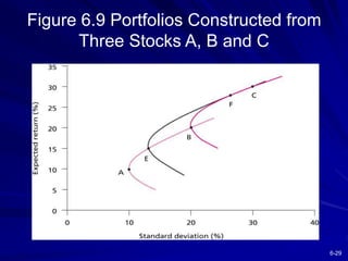
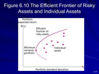
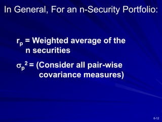
This chapter discusses diversification and portfolio risk. It explains how diversifying across multiple stocks or assets reduces unsystematic risk. The chapter introduces concepts like correlation and covariance that measure how asset returns relate to one another. It shows how optimal portfolios can be created by combining risky assets with a risk-free asset. These portfolios form an efficient frontier that offers the highest expected return for a given level of risk. A single-factor asset pricing model is presented that breaks down risk into systematic and unsystematic components. Finally, the chapter addresses whether risk is reduced when considering long-term stock investments.

1. McGraw-Hill/Irwin © 2008 The McGraw-Hill Companies, Inc., All Rights Reserved.
Efficient Diversification
CHAPTER 6

2. 6-2
6.1 DIVERSIFICATION AND
PORTFOLIO RISK

3. 6-3
Diversification and Portfolio Risk
Market risk
– Systematic or Nondiversifiable
Firm-specific risk
– Diversifiable or nonsystematic

4. 6-4
Figure 6.1 Portfolio Risk as a
Function of the Number of Stocks

5. 6-5
Figure 6.2 Portfolio Risk as a
Function of Number of Securities

6. 6-6
6.2 ASSET ALLOCATION WITH
TWO RISKY ASSETS

7. 6-7
Covariance and Correlation
Portfolio risk depends on the correlation
between the returns of the assets in the
portfolio
Covariance and the correlation coefficient
provide a measure of the returns on two
assets to vary

8. 6-8
Two Asset Portfolio
Return – Stock and Bond
Return
Stock
ht
Stock Weig
Return
Bond
Weight
Bond
Return
Portfolio







S
S
B
B
P
S
S
B
B
p
r
w
r
w
r
r r
w
r
w

9. 6-9
Covariance and Correlation Coefficient
Covariance:
Correlation
Coefficient:
1
( , ) ( ) ( ) ( )
S
S B S S B B
i
Cov r r p i r i r r i r

   
  
   

( , )
S B
SB
S B
Cov r r

 


10. 6-10
Correlation Coefficients:
Possible Values
If  = 1.0, the securities would be
perfectly positively correlated
If  = - 1.0, the securities would be
perfectly negatively correlated
Range of values for  1,2
-1.0 <  < 1.0

11. 6-11
Two Asset Portfolio St Dev –
Stock and Bond
Deviation
Standard
Portfolio
Variance
Portfolio
2
2
,
2
2
2
2
2
2













p
p
S
B
B
S
S
B
S
S
B
B
p w
w
w
w

12. 6-12
rp = Weighted average of the
n securities
p
2 = (Consider all pair-wise
covariance measures)
In General, For an n-Security Portfolio:

13. 6-13
Three Rules of Two-Risky-Asset Portfolios
Rate of return on the portfolio:
Expected rate of return on the portfolio:
P B B S S
r w r w r
 
( ) ( ) ( )
P B B S S
E r w E r w E r
 

14. 6-14
Three Rules of Two-Risky-Asset Portfolios
Variance of the rate of return on the portfolio:
2 2 2
( ) ( ) 2( )( )
P B B S S B B S S BS
w w w w
     
  

15. 6-15
Numerical Text Example: Bond and Stock
Returns (Page 169)
Returns
Bond = 6% Stock = 10%
Standard Deviation
Bond = 12% Stock = 25%
Weights
Bond = .5 Stock = .5
Correlation Coefficient
(Bonds and Stock) = 0

16. 6-16
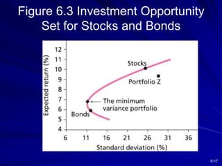
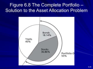
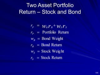
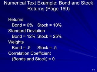
Numerical Text Example: Bond and Stock
Returns (Page 169)
Return = 8%
.5(6) + .5 (10)
Standard Deviation = 13.87%
[(.5)2 (12)2 + (.5)2 (25)2 + …
2 (.5) (.5) (12) (25) (0)] ½
[192.25] ½ = 13.87

17. 6-17
Figure 6.3 Investment Opportunity
Set for Stocks and Bonds

18. 6-18
Figure 6.4 Investment Opportunity Set for
Stocks and Bonds with Various Correlations

19. 6-19
6.3 THE OPTIMAL RISKY PORTFOLIO
WITH A RISK-FREE ASSET

20. 6-20
Extending to Include Riskless Asset
The optimal combination becomes linear
A single combination of risky and riskless
assets will dominate

21. 6-21
Figure 6.5 Opportunity Set Using Stocks
and Bonds and Two Capital Allocation Lines

22. 6-22
Dominant CAL with a Risk-Free
Investment (F)
CAL(O) dominates other lines -- it has the best
risk/return or the largest slope
Slope = ( )
A f
A
E r r



23. 6-23
Dominant CAL with a Risk-Free
Investment (F)
Regardless of risk preferences, combinations of
O & F dominate
( ) ( )
P f A f
P A
E r r E r r
 
 


24. 6-24
Figure 6.6 Optimal Capital Allocation Line
for Bonds, Stocks and T-Bills

25. 6-25
Figure 6.7 The Complete Portfolio

26. 6-26
Figure 6.8 The Complete Portfolio –
Solution to the Asset Allocation Problem

27. 6-27
6.4 EFFICIENT DIVERSIFICATION WITH
MANY RISKY ASSETS

28. 6-28
Extending Concepts to All Securities
The optimal combinations result in lowest
level of risk for a given return
The optimal trade-off is described as the
efficient frontier
These portfolios are dominant

29. 6-29
Figure 6.9 Portfolios Constructed from
Three Stocks A, B and C

30. 6-30
Figure 6.10 The Efficient Frontier of Risky
Assets and Individual Assets

31. 6-31
6.5 A SINGLE-FACTOR ASSET MARKET

32. 6-32
Single Factor Model
βi = index of a securities’ particular return to the
factor
M = unanticipated movement commonly related to
security returns
Ei = unexpected event relevant only to this
security
Assumption: a broad market index like the
S&P500 is the common factor
( )
i i i i
R E R M e

  

33. 6-33
Specification of a Single-Index Model of
Security Returns
Use the S&P 500 as a market proxy
Excess return can now be stated as:
– This specifies the both market and firm risk
i i M
R R e
 
  

34. 6-34
Figure 6.11 Scatter Diagram for Dell

35. 6-35
Figure 6.12 Various Scatter Diagrams

36. 6-36
Components of Risk
Market or systematic risk: risk related to the
macro economic factor or market index
Unsystematic or firm specific risk: risk not
related to the macro factor or market index
Total risk = Systematic + Unsystematic

37. 6-37
Measuring Components of Risk
i
2 = i
2 m
2 + 2(ei)
where;
i
2 = total variance
i
2 m
2 = systematic variance
2(ei) = unsystematic variance

38. 6-38
Total Risk = Systematic Risk + Unsystematic
Risk
Systematic Risk/Total Risk = 2
ßi
2  m
2 / 2 = 2
i
2 m
2 / i
2 m
2 + 2(ei) = 2
Examining Percentage of Variance

39. 6-39
Advantages of the Single Index Model
Reduces the number of inputs for
diversification
Easier for security analysts to specialize

40. 6-40
6.6 RISK OF LONG-TERM INVESTMENTS

41. 6-41
Are Stock Returns Less Risky in the Long
Run?
Consider a 2-year investment
Variance of the 2-year return is double of that of the
one-year return and σ is higher by a multiple of the
square root of 2
1 2
1 2 1 2
2 2
2
Var (2-year total return) = (
( ) ( ) 2 ( , )
0
2 and standard deviation of the return is 2
Var r r
Var r Var r Cov r r
 
 

  
  


42. 6-42
Are Stock Returns Less Risky in the Long
Run?
Generalizing to an investment horizon of n
years and then annualizing:
2
Var(n-year total return) =
Standard deviation ( -year total return) = n
1
(annualized for an - year investment) =
n
n
n n
n n



  

43. 6-43
The Fly in the ‘Time Diversification’
Ointment
Annualized standard deviation is only appropriate
for short-term portfolios
Variance grows linearly with the number of years
Standard deviation grows in proportion to n

44. 6-44
The Fly in the ‘Time Diversification’
Ointment
To compare investments in two different
time periods:
– Risk of the total (end of horizon) rate of return
– Accounts for magnitudes and probabilities