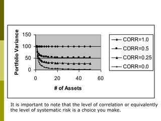
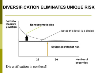
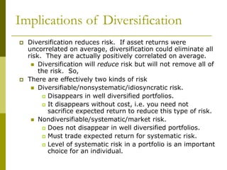
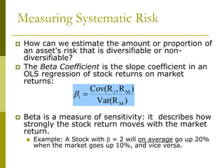
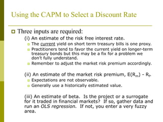
The Capital Asset Pricing Model (CAPM) formalizes the relationship between risk and expected return. It states that the expected return of an asset is determined by its sensitivity to non-diversifiable or systematic risk as measured by its beta. Beta measures how an asset's returns co-vary with the market portfolio. According to CAPM, an asset's expected return is equal to the risk-free rate plus its beta multiplied by the market risk premium. Diversification reduces risk by eliminating asset-specific or diversifiable risk, but not market risk.

1. The Capital Asset Pricing Model
The Risk Return Relation
Formalized

2. Summary
 As we discussed, the “market” pays
investors for two services they provide:
(1) surrendering their capital and
forgoing current consumption and (2)
sharing in the total risk of the economy.
 The first gets you the time value of money.
 The second gets you a risk premium whose
size depends on the share of total risk you
take on.
 From this we found E(R) = Rf + θ
 We refined this to E(R) = Rf + Units × Price

3. Summary
 We needed a reference for measuring risk and
chose the total risk the market has to divide or
the “market portfolio” as that reference.
 The market portfolio is defined to have one unit
of risk (Var(Rm) = 1 unit of risk). Other assets
are evaluated relative to this definition of one
unit of risk.
 From E(R) = Rf + Units × Price we can see that
Price = {E(Rm) – Rf}. (Note: Units = 1 for Rm.)
 In other words we also defined the price per unit
risk (the market risk premium).

4. Summary
 The hard part is to show that any asset’s
contribution to the total risk of the economy or
Var(Rm) is determined not by Var(Ri) but rather
by Cov(Ri, Rm).
 Standardize Cov(Ri, Rm) so that we measure the
risk of each asset relative to our definition of one
unit and we get beta:
βi = Cov(Ri, Rm)/Var(Rm)
 The number of units of risk for asset i is βi.
 So E(Ri)=Rf + βi(E(Rm) – Rf)=Rf + Units × Price.

5. Risk and Return
 When we are concerned with only one asset its
risk and return can be measured, as discussed,
using expected return and variance of return.
 If there is more that one asset (so portfolios
can be formed) risk becomes more complex.
 We will show there are two types of risk for
individual assets:
 Diversifiable/nonsystematic/idiosyncratic risk
 Nondiversifiable/systematic/market risk
 Diversifiable risk can be eliminated without cost
by combining assets into portfolios. (Big Wow.)

6. Diversification
 One of the most important lessons in all of
finance concerns the power of diversification.
 Part of the total risk of any asset can be
“diversified away” (its effect on portfolio risk is
eliminated) without any loss in expected return
(i.e. without cost).
 This also means that no compensation needs to
be provided to investors for exposing their
portfolios to this type of risk.
 Why should the economy pay you to hold risk that you
can get rid of for free (or which is not part of the
aggregate risk that all agents must some how share).
 This in turn implies that the risk/return relation is
actually a systematic risk/return relation.

7. Diversification Example
 Suppose a large green ogre has
approached you and demanded that you
enter into a bet with him.
 The terms are that you must wager
$10,000 and it must be decided by the flip
of a coin, where heads he wins and tails
you win.
 What is your expected payoff and what is
your risk?

8. Example…
 The expected payoff from such a bet is of
course $0 if the coin is fair.
 We can calculate the standard deviation of
this “position” as $10,000, reflecting the
wide swings in value across the two
outcomes (winning and losing).
 Can you suggest another approach that
stays within the rules?

9. Example…
 If instead of wagering the whole $10,000 on one
coin flip think about wagering $1 on each of
10,000 coin flips.
 The expected payoff on this version is still $0 so
you haven’t changed the expectation.
 The standard deviation of the payoff in this
version, however, is $100.
 Why the change?
 If we bet a penny on each of 1,000,000 coin flips,
the risk, measured by the standard deviation of
the payoff, is $10. The expected payoff is of
course still $0.

10. Example…
 The example works so well at reducing risk
because the coin flips are “independent.”
 If the coins were somehow perfectly correlated
we would be right back in the first situation.
 Suppose all flips after the first always landed the same
way, what good is bothering with 10,000 flips?
 With one dollar bets on 10,000 flips, for “flip
correlations” between zero (independence) and
one (perfect correlation) the measure of risk lies
between $100 and $10,000.
 This is one way to see that the way an “asset”
contributes to the risk of a large “portfolio” is
determined by its correlation or covariance with
the other assets in the portfolio.

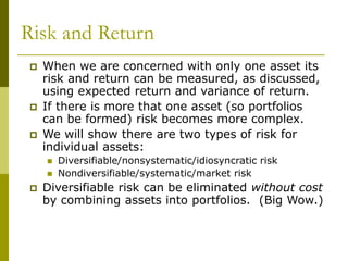
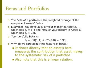
11. Covariances and Correlations: The Keys to
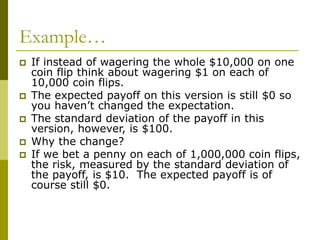
Understanding Diversification
 When thinking in terms of probability
distributions, the covariance between the returns
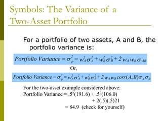
of two assets’ (A & B) equals Cov(A,B) = AB =
 When estimating covariances from historical data,
the estimate is given by:
 Note: An asset’s variance is its covariance with
itself.
p
])
E[R
-
R
])(
E[R
-
R
( s
B
B
A
A
S
1
=
s
s
s

)
R
-
R
)(
R
-
R
(
1
T
1
B
B
A
A
T
1
=
t
t
t



12. Correlation Coefficients
• Covariances are difficult to interpret. Only the
sign is really informative. Is a covariance of 20
big or small?
• The correlation coefficient, , is a normalized
version of the covariance given by:
• Correlation = CORR(A,B) =
• The correlation will always lie between 1 and -1.
 A correlation of 1.0 implies ...
 A correlation of -1.0 implies ...
 A correlation of 0.0 implies ...
AB
B
A
AB
B
A







=
B)
Cov(A,

13. Return (%) Deviation from mean Squared Dev. from Mean
Probability A B P A B P A*B A B P
0.2 18 25 21.5 2 13 7.5 26 4 169 56.25
0.2 30 10 20 14 -2 6 -28 196 4 36
0.2 -10 10 0 -26 -2 -14 52 676 4 196
0.2 25 20 22.5 9 8 8.5 72 81 64 72.25
0.2 17 -5 6 1 -17 -8 -17 1 289 64
Mean 16 12 14 21 191.6 106 84.9
Risk and Return in Portfolios: Example
•Two Assets, A and B
•A portfolio, P, comprised of 50% of your total investment
invested in asset A and 50% in B.
•There are five equally probable future outcomes, see below.
In this case:
•VAR(RA) = 191.6, STD(RA) = 13.84, and E(RA) = 16%.
•VAR(RB) = 106.0, STD(RB) = 10.29, and E(RB) = 12%.
•COV(RA, RB) = 21
•CORR(RA, RB) = 21/(13.84*10.29) = .1475.
•VAR(RP)=84.9, STD(Rp)=9.21, E(Rp)=½ E(RA) + ½ E(RB)=14%
•Var(Rp) or STD(RP) is less than that of either component!

14. What risk return combinations would be possible with
different weights?
CORR(AB) 0.1475
-0.5
Risk and Return in 2-asset Portfolio
11
12
13
14
15
16
17
0 2 4 6 8 10 12 14 16
Standard Deviation
Expected
Return
Asset A
Asset B
•
•
•
½ and ½ portfolio

15. CORR(AB) 0.1 -1 1
-0.5
Risk and Return in 2-asset Portfolio
11
12
13
14
15
16
17
0 2 4 6 8 10 12 14 16
Standard Deviation
Expected
Return
Asset A
Asset B •
•
What risk return combinations would be possible with a
different correlation between A and B?

16. Symbols: The Variance of a
Two-Asset Portfolio
For a portfolio of two assets, A and B, the
portfolio variance is:



 AB
B
A
2
B
2
B
2
A
2
A
2
p w
w
2
+
w
+
w
=
Variance
Portfolio 
For the two-asset example considered above:
Portfolio Variance = .52(191.6) + .52(106.0)
+ 2(.5)(.5)21
= 84.9 (check for yourself)
Or,
B
A
B
A
2
B
2
B
2
A
2
A
2
p B
A
corr
w
w
2
+
w
+
w
=
Variance
Portfolio 



 )
,
(


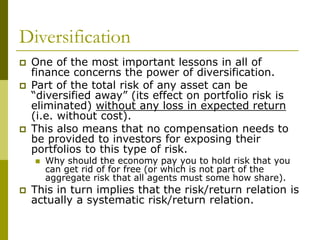
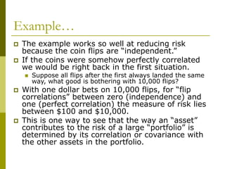
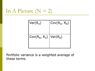
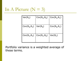
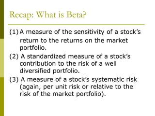
17. For General Portfolios
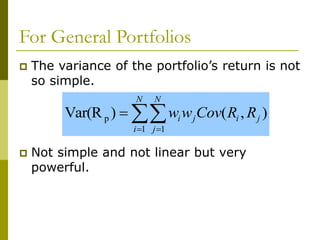
• The expected return on a portfolio is the
weighted average of the expected returns
on each asset. If wi is the proportion of
the investment invested in asset i, then



N
i
i
i R
E
w
1
p ]
[
]
E[R
• Note that this is a ‘linear’ relationship.

18. For General Portfolios
 The variance of the portfolio’s return is not
so simple.
 Not simple and not linear but very
powerful.

 

N
i
N
j
j
i
j
i R
R
Cov
w
w
1 1
p )
,
(
)
Var(R

19. In A Picture (N = 2)
Var(RA) Cov(RA, RB)
Cov(RB, RA) Var(RB)
Portfolio variance is a weighted average of
these terms.

20. In A Picture (N = 3)
Portfolio variance is a weighted average of
these terms.
Var(RA) Cov(RA,RB) Cov(RA,RC)
Cov(RB,RA) Var(RB) Cov(RB,RC)
Cov(RC,RA) Cov(RC,RB) Var(RC)

21. In A Picture (N = 10)
Portfolio variance is a simple weighted average of
the terms in the squares. The blue are covariances
and the white the variance terms.

22. In A Picture (N = 20)
Which squares are becoming more important?

23. 0
50
100
150
0 20 40 60
# of Assets
Portfolio
Variance
CORR=1.0
CORR=0.5
CORR=0.25
CORR=0.0
It is important to note that the level of correlation or equivalently
the level of systematic risk is a choice you make.

24. DIVERSIFICATION ELIMINATES UNIQUE RISK
Nonsystematic risk
Systematic/Market risk
Number of
securities
25 50
Diversification is costless!!
Note: this level is a choice
Portfolio
Standard
Deviation

25. Implications of Diversification
 Diversification reduces risk. If asset returns were
uncorrelated on average, diversification could eliminate all
risk. They are actually positively correlated on average.
 Diversification will reduce risk but will not remove all of
the risk. So,
 There are effectively two kinds of risk
 Diversifiable/nonsystematic/idiosyncratic risk.
 Disappears in well diversified portfolios.
 It disappears without cost, i.e. you need not
sacrifice expected return to reduce this type of risk.
 Nondiversifiable/systematic/market risk.
 Does not disappear in well diversified portfolios.
 Must trade expected return for systematic risk.
 Level of systematic risk in a portfolio is an important
choice for an individual.

26. Nonsystematic/diversifiable risks
 Examples
 Firm discovers a gold mine beneath its
property
 Lawsuits
 Technological innovations
 Labor strikes
 The key is that these events are random and
unrelated across firms. For the assets in a
portfolio, some surprises are positive, some
are negative. On average, across assets, the
surprises offset each other if your portfolio is
made up of a large number of assets.

27. Systematic/Nondiversifiable risk
 We know that the returns on different assets
are positively correlated with each other on
average. This suggests that economy-wide
influences affect all assets.
 Examples:
 Business Cycle
 Inflation Shocks
 Productivity Shocks
 Interest Rate Changes
 Major Technological Change
 These are economic events that affect all
assets. The risk associated with these events
is systematic (system wide), and does not
disappear in well diversified portfolios.

28. Measuring Systematic Risk
 How can we estimate the amount or proportion of
an asset's risk that is diversifiable or non-
diversifiable?
 The Beta Coefficient is the slope coefficient in an
OLS regression of stock returns on market
returns:
 Beta is a measure of sensitivity: it describes how
strongly the stock return moves with the market
return.
 Example: A Stock with  = 2 will on average go up 20%
when the market goes up 10%, and vice versa.
)
Var(R
)
R
,
Cov(R
M
M
i
i 


29. Betas and Portfolios
 The Beta of a portfolio is the weighted average of the
component assets’ Betas.
 Example: You have 30% of your money in Asset X,
which has X = 1.4 and 70% of your money in Asset Y,
which has Y = 0.8.
 Your portfolio Beta is:
P = .30(1.4) + .70(0.8) = 0.98.
 Why do we care about this feature of betas?
 It shows directly that an asset’s beta
measures the contribution that asset makes
to the systematic risk of a portfolio!
 Also note that this is a linear relation.

30. Recap: What is Beta?
(1) A measure of the sensitivity of a stock’s
return to the returns on the market
portfolio.
(2) A standardized measure of a stock’s
contribution to the risk of a well
diversified portfolio.
(3) A measure of a stock’s systematic risk
(again, per unit risk or relative to the
risk of the market portfolio).

31. How To Get Beta.
 We estimate beta using a regression equation.
 In practice, generally use last five years of
monthly data. Some companies publish
beta estimates on a regular basis:
 Value Line, Merrill Lynch Beta Book, S&P
 What if the company is not publicly traded?
 Find a comparable company that is traded.
 Use accounting data (ROE) instead of stock
returns.
 Reason it out.

32. What Determines Beta?
 Beta is a measure of sensitivity to the market.
 Companies with cyclical cash flows will tend to
have higher betas.
 Higher operating leverage implies higher betas.
Operating leverage is the ratio of fixed costs to
variable costs.
 Higher financial leverage also means a higher
equity beta (more on this later).

33. The Capital Asset Pricing Model (CAPM)
 Given that
 some risk can be diversified,
 diversification is easy and costless,
 rational investors diversify,
 There should be no premium associated with
diversifiable risk.
 The question becomes: What is the
equilibrium relation between systematic risk
and expected return in the capital markets?
 The CAPM is the best-known and most-widely
used equilibrium model of the risk/return
(systematic risk/return) relation.

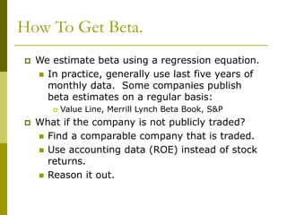
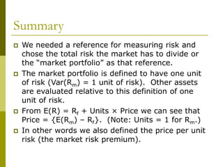
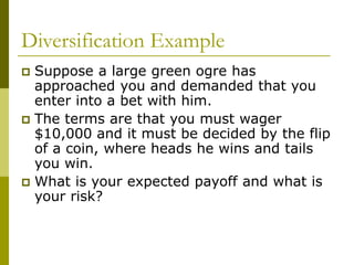
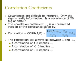
34. CAPM Intuition: Recap
 E[Ri] = RF (risk free rate) + Risk Premium
= Appropriate Discount Rate
 Risk free assets earn the risk-free rate (think
of this as a rental rate on capital).
 If the asset is risky, we need to add a risk
premium.
 The size of the risk premium depends on the amount
of systematic risk for the asset (stock, bond, or
investment project) and the price per unit risk.
 Could a risk premium ever be negative?

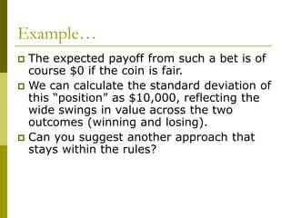
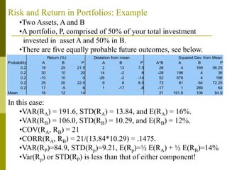
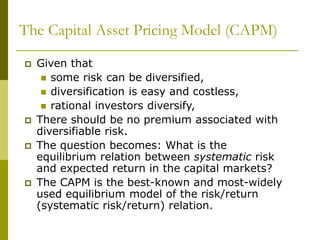
35. The CAPM Intuition Formalized
]
R
]
[E[R
)
Var(R
)
R
,
Cov(R
R
]
E[R F
M
M
M
i
F
i 


]
R
]
[E[R
R
]
E[R F
M
i
F
i 

 
• The expression above is referred to as the “Security
Market Line” (SML).
Number of units of
systematic risk () Market Risk Premium
or the price per unit risk
or,

36. Using the CAPM to Select a Discount Rate
 Three inputs are required:
(i) An estimate of the risk free interest rate.
 The current yield on short term treasury bills is one proxy.
 Practitioners tend to favor the current yield on longer-term
treasury bonds but this may be a fix for a problem we
don’t fully understand.
 Remember to adjust the market risk premium accordingly.
(ii) An estimate of the market risk premium, E(Rm) - Rf.
 Expectations are not observable.
 Generally use a historically estimated value.
(iii) An estimate of beta. Is the project or a surrogate
for it traded in financial markets? If so, gather data and
run an OLS regression. If not, you enter a very fuzzy
area.

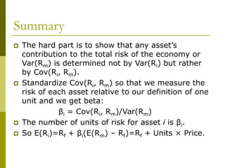
37. The Market Risk Premium
 The market is defined as a portfolio of all wealth including real
estate, human capital, etc.
 In practice, a broad based stock index, such as the S&P 500 or
the portfolio of all NYSE stocks, is generally used.
]
R
]
[E[R F
M 
The Market Risk Premium Is Defined As:
 Historically, the market risk premium has been about 8.5% - 9%
above the return on treasury bills.
 The market risk premium has been about 6.5% - 7% above the
return on treasury bonds.

38. Problems
 The current risk free rate is 4% and the expected
risk premium on the market portfolio is 7%.
 An asset has a beta of 1.2. What is the expected return
on this asset? Interpret the number 1.2.
 An asset has a beta of 0.6. What is the expected return
on this asset?
 If we invest ½ of our money in the first asset and ½ of
our money in the second, what is our portfolio beta and
what is its expected return?
 Relative to the first asset our portfolio has a smaller
expected return, why?
 Does this mean the first asset is better than the
portfolio?

39. Problem
 The current risk free rate is 4% and the expected
risk premium on the market portfolio is 7%.
 You work for a software company and have been asked
to estimate the appropriate discount rate for a proposed
investment project.
 Your company’s stock has a beta of 1.3.
 The project is a proposal to begin cigarette production.
 RJR Reynolds has a beta of 0.22.
 What is the appropriate discount rate and why?