This document discusses various models for valuing equity, including balance sheet models, dividend discount models, and price/earnings ratios. It describes the constant growth model and multi-stage growth models in detail. It also discusses using free cash flow approaches and comparing intrinsic value to market price. Overall, the document provides an overview of fundamental approaches to valuing stocks.

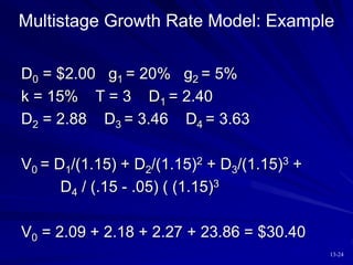
1. McGraw-Hill/Irwin © 2008 The McGraw-Hill Companies, Inc., All Rights Reserved.
Equity Valuation
CHAPTER 13

2. 13-2
13.1 VALUATION BY COMPARABLES

3. 13-3
Fundamental Stock Analysis:
Models of Equity Valuation
Basic Types of Models
– Balance Sheet Models
– Dividend Discount Models
– Price/Earnings Ratios
Estimating Growth Rates and
Opportunities

4. 13-4
Models of Equity Valuation
Valuation models use comparables
– Look at the relationship between price and various
determinants of value for similar firms
The internet provides a convenient way to
access firm data. Some examples are:
– EDGAR
– Finance.yahoo.com

5. 13-5
Table 13.1 Microsoft Corporation Financial
Highlights

6. 13-6
Valuation Methods
Book value
Market value
Liquidation value
Replacement cost

7. 13-7
13.2 INTRINSIC VALUE VERSUS
MARKET PRICE

8. 13-8
Expected Holding Period Return
The return on a stock investment comprises cash
dividends and capital gains or losses
– Assuming a one-year holding period
 
1 1 0
0
( ) ( )
Expected HPR= ( )
E D E P P
E r
P
 


9. 13-9
Required Return
CAPM gave us required return:
If the stock is priced correctly
– Required return should equal expected return
( )
f M f
k r E r r
  
  
 

10. 13-10
Intrinsic Value and Market Price
Market Price
– Consensus value of all potential traders
– Current market price will reflect intrinsic value
estimates
– This consensus value of the required rate of return, k,
is the market capitalization rate
Trading Signal
– IV > MP Buy
– IV < MP Sell or Short Sell
– IV = MP Hold or Fairly Priced

11. 13-11
13.3 DIVIDEND DISCOUNT MODELS

12. 13-12
General Model
V
D
k
o
t
t
t




( )
1
1
V0 = Value of Stock
Dt = Dividend
k = required return

13. 13-13
No Growth Model
V
D
k
o 
Stocks that have earnings and dividends
that are expected to remain constant
– Preferred Stock

14. 13-14
No Growth Model: Example
E1 = D1 = $5.00
k = .15
V0 = $5.00 / .15 = $33.33
V
D
k
o 

15. 13-15
Constant Growth Model
Vo
D g
k g
o



( )
1
g = constant perpetual growth rate

16. 13-16
Constant Growth Model: Example
Vo
D g
k g
o



( )
1
E1 = $5.00 b = 40% k = 15%
(1-b) = 60% D1 = $3.00 g = 8%
V0 = 3.00 / (.15 - .08) = $42.86

17. 13-17
Stock Prices and Investment Opportunities
g ROE b
 
g = growth rate in dividends
ROE = Return on Equity for the firm
b = plowback or retention percentage rate
– (1- dividend payout percentage rate)

18. 13-18
Figure 13.1 Dividend Growth for
Two Earnings Reinvestment Policies

19. 13-19
Present Value of Growth Opportunities
If the stock price equals its IV, growth rate is
sustained, the stock should sell at:
If all earnings paid out as dividends, price should
be lower (assuming growth opportunities exist)
1
0
D
P
k g



20. 13-20
Present Value of Growth Opportunities
(cont.)
Price = No-growth value per share + PVGO
(present value of growth opportunities)
Where:
E1 = Earnings Per Share for period 1 and
1
0
E
P PVGO
k
 
0 1
(1 )
( )
D g E
PVGO
k g k

 


21. 13-21
Partitioning Value: Example
ROE = 20% d = 60% b = 40%
E1 = $5.00 D1 = $3.00 k = 15%
g = .20 x .40 = .08 or 8%

22. 13-22
P
NGV
PVGO
o
o



 
  
3
15 08
86
5
15
33
86 33 52
(. . )
$42.
.
$33.
$42. $33. $9.
Partitioning Value: Example (cont.)
Po = price with growth
NGVo = no growth component value
PVGO = Present Value of Growth Opportunities

23. 13-23
Life Cycles and Multistage Growth Models
P D
g
k
D g
k g k
o o
t
t
t
T
T
T





 

( )
( )
( )
( )( )
1
1
1
1
1
1
2
2
g1 = first growth rate
g2 = second growth rate
T = number of periods of growth at g1

24. 13-24
Multistage Growth Rate Model: Example
D0 = $2.00 g1 = 20% g2 = 5%
k = 15% T = 3 D1 = 2.40
D2 = 2.88 D3 = 3.46 D4 = 3.63
V0 = D1/(1.15) + D2/(1.15)2 + D3/(1.15)3 +
D4 / (.15 - .05) ( (1.15)3
V0 = 2.09 + 2.18 + 2.27 + 23.86 = $30.40

25. 13-25
13.4 PRICE-EARNINGS RATIOS

26. 13-26
P/E Ratio and Growth Opportunities
P/E Ratios are a function of two factors
– Required Rates of Return (k)
– Expected growth in Dividends
Uses
– Relative valuation
– Extensive use in industry

27. 13-27
P/E Ratio: No expected growth
P
E
k
P
E k
0
1
0
1
1


E1 - expected earnings for next year
– E1 is equal to D1 under no growth
k - required rate of return

28. 13-28
P/E Ratio: Constant Growth
P
D
k g
E b
k b ROE
P
E
b
k b ROE
0
1 1
0
1
1
1




 


 
( )
( )
( )
b = retention ration
ROE = Return on Equity

29. 13-29
Numerical Example: No Growth
E0 = $2.50 g = 0 k = 12.5%
P0 = D/k = $2.50/.125 = $20.00
P/E = 1/k = 1/.125 = 8

30. 13-30
Numerical Example with Growth
b = 60% ROE = 15% (1-b) = 40%
E1 = $2.50 (1 + (.6)(.15)) = $2.73
D1 = $2.73 (1-.6) = $1.09
k = 12.5% g = 9%
P0 = 1.09/(.125-.09) = $31.14
P/E = 31.14/2.73 = 11.4
P/E = (1 - .60) / (.125 - .09) = 11.4

31. 13-31
P/E Ratios and Stock Risk
Riskier stocks will have lower P/E multiples
Riskier firms will have higher required rates of
return (higher values of k)
1
P b
E k g




32. 13-32
Pitfalls in Using P/E Ratios
Flexibility in reporting makes choice of
earnings difficult
Pro forma earnings may give a better
measure of operating earnings
Problem of too much flexibility

33. 13-33
Figure 13.3 P/E Ratios and Inflation

34. 13-34
Figure 13.4 Earnings Growth
for Two Companies

35. 13-35
Figure 13.5 Price-Earnings Ratios

36. 13-36
Figure 13.6 P/E Ratios

37. 13-37
Other Comparative Valuation Ratios
Price-to-book
Price-to-cash flow
Price-to-sales
Be creative

38. 13-38
Figure 13.7 Valuation Ratios for the S&P
500

39. 13-39
13.5 FREE CASH FLOW VALUATION
APPROACHES

40. 13-40
Free Cash Flow
One approach is to discount the free cash
flow for the firm (FCFF) at the weighted-
average cost of capital
– Subtract existing value of debt
– FCFF = EBIT (1- tc) + Depreciation – Capital
expenditures – Increase in NWC
where:
EBIT = earnings before interest and taxes
tc = the corporate tax rate
NWC = net working capital

41. 13-41
Free Cash Flow (cont.)
Another approach focuses on the free
cash flow to the equity holders (FCFE) and
discounts the cash flows directly at the
cost of equity
FCFE = FCFF – Interest expense (1- tc) +
Increases in net debt

42. 13-42
Comparing the Valuation Models
Free cash flow approach should provide
same estimate of IV as the dividend
growth model
In practice the two approaches may differ
substantially
– Simplifying assumptions are used

43. 13-43
13.6 THE AGGREGATE STOCK MARKET

44. 13-44
Earnings Multiplier Approach
Forecast corporate profits for the coming
period
Derive an estimate for the aggregate P/E
ratio using long-term interest rates
Product of the two forecasts is the
estimate of the end-of-period level of the
market

45. 13-45
Figure 13.8 Earnings Yield of the S&P 500
Versus 10-year Treasury Bond Yield

46. 13-46
Table 13.4 S&P 500 Index Forecasts