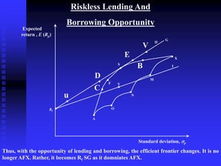
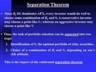
This chapter discusses portfolio theory and the benefits of diversification. It introduces the concept of the efficient frontier, which graphs the set of optimal portfolios that maximize expected return for a given level of risk. The chapter also discusses measuring risk and return of portfolios, the single index model, and how introducing a risk-free borrowing and lending opportunity shifts the efficient frontier. The optimal portfolio is found where the efficient frontier is tangent to an investor's indifference curve.

1. Chapter 7
PORTFOLIO THEORY
The Benefits of Diversification

2. OUTLINE
• Portfolio Return and Risk
• Measurement of Comovements in Security Returns
• Calculation of Portfolio Risk
• Efficient Frontier
• Optimal Portfolio
• Riskless Lending and Borrowing
• The Single Index Model

3. Portfolio Expected Return
n
E(RP) =  wi E(Ri)
i=1
where E(RP) = expected portfolio return
wi = weight assigned to security i
E(Ri) = expected return on security i
n = number of securities in the portfolio
Example A portfolio consists of four securities with expected returns
of 12%, 15%, 18%, and 20% respectively. The proportions of
portfolio value invested in these securities are 0.2, 0.3, 0.3, and 0.20
respectively.
The expected return on the portfolio is:
E(RP) = 0.2(12%) + 0.3(15%) + 0.3(18%) + 0.2(20%)
= 16.3%

4. Portfolio Risk
The risk of a portfolio is measured by the variance (or
standard deviation) of its return. Although the expected
return on a portfolio is the weighted average of the
expected returns on the individual securities in the
portfolio, portfolio risk is not the weighted average of the
risks of the individual securities in the portfolio (except
when the returns from the securities are uncorrelated).

5. Measurement Of Comovements
In Security Returns
• To develop the equation for calculating portfolio risk we
need information on weighted individual security risks
and weighted comovements between the returns of
securities included in the portfolio.
• Comovements between the returns of securities are
measured by covariance (an absolute measure) and
coefficient of correlation (a relative measure).

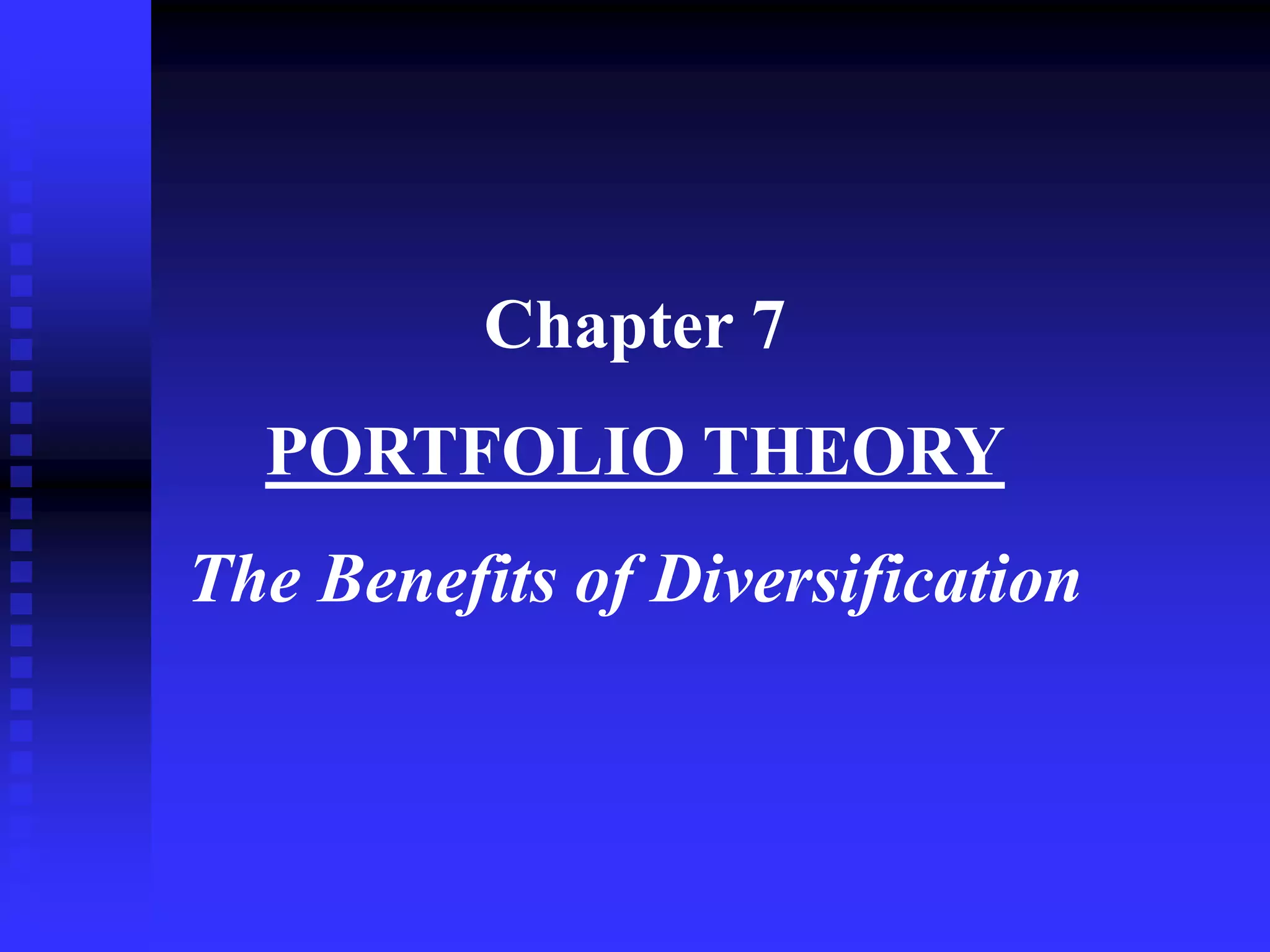
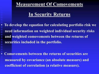
6. Covariance
COV (Ri , Rj) = p1 [Ri1 – E(Ri)] [ Rj1 – E(Rj)]
+ p2 [Ri2 – E(Rj)] [Rj2 – E(Rj)]
+
+ pn [Rin – E(Ri)] [Rjn – E(Rj)]
•
•
•
•

7. Illustration
The returns on assets 1 and 2 under five possible states of nature are given below
State of nature Probability Return on asset 1 Return on asset 2
1 0.10 -10% 5%
2 0.30 15 12
3 0.30 18 19
4 0.20 22 15
5 0.10 27 12
The expected return on asset 1 is :
E(R1) = 0.10 (-10%) + 0.30 (15%) + 0.30 (18%) + 0.20 (22%) + 0.10 (27%) = 16%
The expected return on asset 2 is :
E(R2) = 0.10 (5%) + 0.30 (12%) + 0.30 (19%) + 0.20 (15%) + 0.10 (12%) = 14%
The covariance between the returns on assets 1 and 2 is calculated below :

8. State of
nature
(1)
Probability
(2)
Return on
asset 1
(3)
Deviation of
the return on
asset 1 from its
mean
(4)
Return on
asset 2
(5)
Deviation of
the return on
asset 2 from
its mean
(6)
Product of the
deviations
times
probability
(2) x (4) x (6)
1 0.10 -10% -26% 5% -9% 23.4
2 0.30 15% -1% 12% -2% 0.6
3 0.30 18% 2% 19% 5% 3.0
4 0.20 22% 6% 15% 1% 1.2
5 0.10 27% 11% 12% -2% -2.2
Sum = 26.0
Thus the covariance between the returns on the two assets is 26.0.

9. Coefficient Of Correlation
Cov (Ri , Rj)
Cor (Ri , Rj) or ij =
 (Ri , Rj)
ij
i j
ij = ij . i . j
where ij = correlation coefficient between the returns on
securities i and j
ij = covariance between the returns on securities
i and j
i , j = standard deviation of the returns on securities
i and j
=

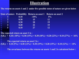
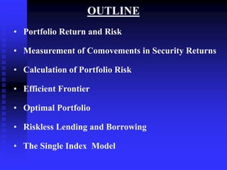
10. Portfolio Risk : 2 – Security Cas
p = [w1
2 1
2 + w2
2 2
2 + 2w1w2 12 1 2]½
Example : w1 = 0.6 , w2 = 0.4,
1 = 10%, 2 = 16%
12 = 0.5
p = [0.62 x 102 + 0.42 x 162 +2 x 0.6 x 0.4 x 0.5 x 10 x 16]½
= 10.7%

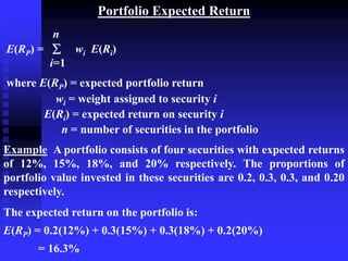
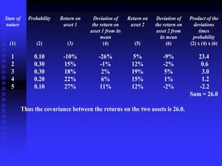
11. Portfolio Risk : n – Security Case
p = [   wi wj ij i j ] ½
Example : w1 = 0.5 , w2 = 0.3, and w3 = 0.2
1 = 10%, 2 = 15%, 3 = 20%
12 = 0.3, 13 = 0.5, 23 = 0.6
p = [w1
2 1
2 + w2
2 2
2 + w3
2 3
2 + 2 w1 w2 12 1 2
+ 2w2 w3 13 1 3 + 2w2 w3 232 3] ½
= [0.52 x 102 + 0.32 x 152 + 0.22 x 202
+ 2 x 0.5 x 0.3 x 0.3 x 10 x 15
+ 2 x 0.5 x 0.2 x 05 x 10 x 20
+ 2 x 0.3 x 0.2 x 0.6 x 15 x 20] ½
= 10.79%

12. Risk Of An N - Asset Portfolio
2
p =   wi wj ij i j
n x n MATRIX
1 2 3 … n
1 w1
2
σ1
2
w1w2ρ12σ1σ2 w1w3ρ13σ1σ3 … w1wnρ1nσ1σn
2 w2w1ρ21σ2σ1 w2
2
σ2
2
w2w3ρ23σ2σ3 … w2wnρ2nσ2σn
3 w3w1ρ31σ3σ1 w3w2ρ32σ3σ2 w3
2
σ3
2
…
: : :
n wnw1ρn1σnσ1 wn
2
σn
2

13. Dominance Of Covariance
As the number of securities included in a portfolio
increases, the importance of the risk of each individual
security decreases whereas the significance of the
covariance relationship increases.

14. Portfolio Proportion of A
wA
Proportion of B
wB
Expected return
E (Rp)
Standard deviation
p
1 (A) 1.00 0.00 12.00% 20.00%
2 0.90 0.10 12.80% 17.64%
3 0.759 0.241 13.93% 16.27%
4 0.50 0.50 16.00% 20.49%
5 0.25 0.75 18.00% 29.41%
6 (B) 0.00 1.00 20.00% 40.00%
Efficient Frontier
For A Two Security-Case
Security A Security B
Expected return 12% 20%
Standard deviation 20% 40%
Coefficient of correlation -0.2

15. Portfolio Options And
The Efficient Frontier
•
•
12%
20%
20% 40%
Risk, p
Expected
return , E(Rp)
1 (A)
6 (B)
2
3

16. Feasible Frontier Under Various Degrees Of Coefficient of
Correlation
•
12%
20%
A (WA = 1)
Standard deviation, p
Expected
return , E (Rp)
B (WB = 1)

17. Efficient Frontier For The
n-Security Case
Standard deviation, p
Expected
return , E (Rp)
A
O
N
M
X
F
•
•
•
•
•
B
D
Z•
•
•

18. Optimal Portfolio
•
•
•
•
•
•
P*
Q*
A
O
N
M
X
Standard deviation, p
Expected
return , E (Rp)
IQ3
IQ2
IQ1
IP3 IP2 IP1

19. •
•
•
•
•
•
A
O
N
M
X
Standard deviation, p
Expected
return , E (Rp)
•
•
•
•
•
•
• •
Rf
u
D
E
V
G
B
C
F Y
I
II
•
S
Riskless Lending And
Borrowing Opportunity
Thus, with the opportunity of lending and borrowing, the efficient frontier changes. It is no
longer AFX. Rather, it becomes Rf SG as it domniates AFX.

20. Separation Theorem
• Since Rf SG dominates AFX, every investor would do well to
choose some combination of Rf and S. A conservative investor
may choose a point like U, whereas an aggressive investor may
choose a point like V.
• Thus, the task of portfolio selection can be separated into two
steps:
1. Identification of S, the optimal portfolio of risky securities.
2. Choice of a combination of Rf and S, depending on one’s
risk attitude.
This is the import of the celebrated separation theorem

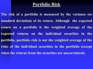
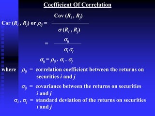
21. Single Index Model
INFORMATION - INTENSITY OF THE MARKOWITZ MODEL
n SECURITIES
n VARIANCE TERMS & n(n -1) /2
COVARIANCE TERMS
SHARPE’S MODEL
Rit = ai + bi RMt + eit
E(Ri) = ai + bi E(RM)
VAR (Ri) = bi
2 [VAR (RM)] + VAR (ei)
COV (Ri ,Rj) = bi bj VAR (RM)
MARKOWITZ MODEL SINGLE INDEX MODEL
n (n + 3)/2 3n + 2
E (Ri) & VAR (Ri) FOR EACH bi , bj VAR (ei) FOR
SECURITY n( n - 1)/2 EACH SECURITY &
COVARIANCE TERMS E (RM) & VAR (RM)

22. SUMMING UP
• Portfolio theory, originally proposed by Markowitz, is the
first formal attempt to quantify the risk of a portfolio and
develop a methodology for determining the optimal portfolio.
• The expected return on a portfolio of n securities is :
E(Rp) =  wi E(Ri)
• The variance and standard deviation of the return on an
n-security portfolio are:
p
2 =   wi wj ij i j
p =   wi wj ij i j
½
• A portfolio is efficient if (and only if) there is an alternative
with (i) the same E(Rp) and a lower p or (ii) the same p and
a higher E(Rp), or (iii) a higher E(Rp) and a lower p

23. • Given the efficient frontier and the risk-return indifference
curves, the optimal portfolio is found at the tangency
between the efficient frontier and a utility indifference curve.
• If we introduce the opportunity for lending and borrowing at
the risk-free rate, the efficient frontier changes dramatically.
It is simply the straight line from the risk-free rate which is
tangential to the broken-egg shaped feasible region
representing all possible combinations of risky assets.
• The Markowitz model is highly information-intensive.
• The single index model, proposed by sharpe, is a very helpful
simplification of the Markowitz model.