Here are the SQL commands for the questions:
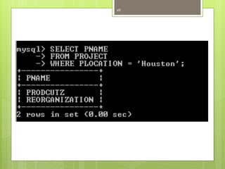
Q1: SELECT PNAME FROM PROJECT WHERE PLOCATION='Houston';
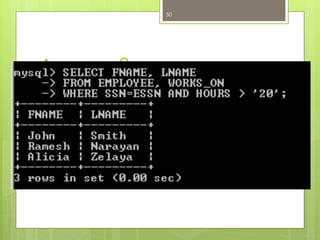
Q2: SELECT FNAME, LNAME FROM EMPLOYEE WHERE HOURS>20;
Q3: SELECT FNAME, LNAME FROM EMPLOYEE, DEPARTMENT WHERE MGRSSN=SSN;
Course Learning Outcome
› CLO1 : Explain the fundamentals
concepts of database management and
relational data model to create a
database based on an organization’s
requirements.
› CLO3 : Solve an organization’s
requirements by selecting the correct
database query formulation using an
appropriate commercial Database
Management System (DBMS).
3.
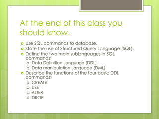
At the endof this class you
should know.
› Use SQL commands to database.
› State the use of Structured Query Language (SQL).
› Define the two main sublanguages in SQL
commands:
a. Data Definition Language (DDL)
b. Data manipulation Language (DML)
› Describe the functions of the four basic DDL
commands:
a. CREATE
b. USE
c. ALTER
d. DROP
4.
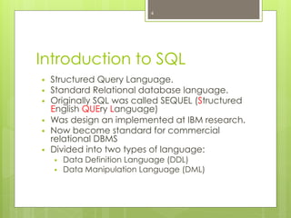
Introduction to SQL
§ Structured Query Language.
§ Standard Relational database language.
§ Originally SQL was called SEQUEL (Structured
English QUEry Language)
§ Was design an implemented at IBM research.
§ Now become standard for commercial
relational DBMS
§ Divided into two types of language:
§ Data Definition Language (DDL)
§ Data Manipulation Language (DML)
4
5.
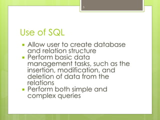
Use of SQL
¡ Allow user to create database
and relation structure
¡ Perform basic data
management tasks, such as the
insertion, modification, and
deletion of data from the
relations
¡ Perform both simple and
complex queries
5
6.
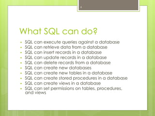
What SQL cando?
§ SQL can execute queries against a database
§ SQL can retrieve data from a database
§ SQL can insert records in a database
§ SQL can update records in a database
§ SQL can delete records from a database
§ SQL can create new databases
§ SQL can create new tables in a database
§ SQL can create stored procedures in a database
§ SQL can create views in a database
§ SQL can set permissions on tables, procedures,
and views
6
7.
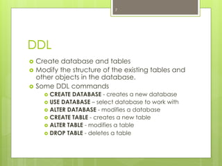
DDL
› Create databaseand tables
› Modify the structure of the existing tables and
other objects in the database.
› Some DDL commands
› CREATE DATABASE - creates a new database
› USE DATABASE – select database to work with
› ALTER DATABASE - modifies a database
› CREATE TABLE - creates a new table
› ALTER TABLE - modifies a table
› DROP TABLE - deletes a table
7
8.
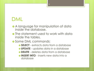
DML
› A languagefor manipulation of data
inside the database.
› The statement used to work with data
inside the tables.
› Some DML commands:
› SELECT - extracts data from a database
› UPDATE - updates data in a database
› DELETE - deletes data from a database
› INSERT INTO - inserts new data into a
database
8
9.
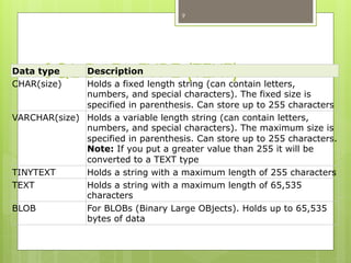
SQL DATA TYPE(TEXT)
9
Data type Description
CHAR(size) Holds a fixed length string (can contain letters,
numbers, and special characters). The fixed size is
specified in parenthesis. Can store up to 255 characters
VARCHAR(size) Holds a variable length string (can contain letters,
numbers, and special characters). The maximum size is
specified in parenthesis. Can store up to 255 characters.
Note: If you put a greater value than 255 it will be
converted to a TEXT type
TINYTEXT Holds a string with a maximum length of 255 characters
TEXT Holds a string with a maximum length of 65,535
characters
BLOB For BLOBs (Binary Large OBjects). Holds up to 65,535
bytes of data
10.
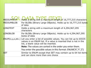
SQL DATA TYPE(TEXT)MEDIUMTEXT Holds a string with a maximum length of 16,777,215 characters
MEDIUMBLOB For BLOBs (Binary Large OBjects). Holds up to 16,777,215 bytes
of data
LONGTEXT Holds a string with a maximum length of 4,294,967,295
characters
LONGBLOB For BLOBs (Binary Large OBjects). Holds up to 4,294,967,295
bytes of data
ENUM(x,y,z,etc.) Let you enter a list of possible values. You can list up to 65535
values in an ENUM list. If a value is inserted that is not in the
list, a blank value will be inserted.
Note:
The
values
are
sorted
in
the
order
you
enter
them.
You
enter
the
possible
values
in
this
format:
ENUM('X','Y','Z')
SET Similar to ENUM except that SET may contain up to 64 list items
and can store more than one choice
10
11.
SQL DATA TYPE(NUMBER)
11
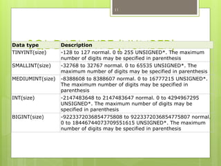
Data type Description
TINYINT(size) -128 to 127 normal. 0 to 255 UNSIGNED*. The maximum
number of digits may be specified in parenthesis
SMALLINT(size) -32768 to 32767 normal. 0 to 65535 UNSIGNED*. The
maximum number of digits may be specified in parenthesis
MEDIUMINT(size) -8388608 to 8388607 normal. 0 to 16777215 UNSIGNED*.
The maximum number of digits may be specified in
parenthesis
INT(size) -2147483648 to 2147483647 normal. 0 to 4294967295
UNSIGNED*. The maximum number of digits may be
specified in parenthesis
BIGINT(size) -9223372036854775808 to 9223372036854775807 normal.
0 to 18446744073709551615 UNSIGNED*. The maximum
number of digits may be specified in parenthesis
12.
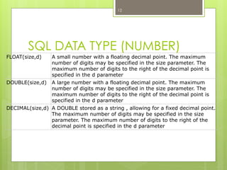
SQL DATA TYPE(NUMBER)
FLOAT(size,d) A small number with a floating decimal point. The maximum
number of digits may be specified in the size parameter. The
maximum number of digits to the right of the decimal point is
specified in the d parameter
DOUBLE(size,d) A large number with a floating decimal point. The maximum
number of digits may be specified in the size parameter. The
maximum number of digits to the right of the decimal point is
specified in the d parameter
DECIMAL(size,d) A DOUBLE stored as a string , allowing for a fixed decimal point.
The maximum number of digits may be specified in the size
parameter. The maximum number of digits to the right of the
decimal point is specified in the d parameter
12
13.
SQL DATA TYPE(DATE)
13
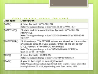
Data type Description
DATE() A date. Format: YYYY-MM-DD
Note: The supported range is from '1000-01-01' to '9999-12-31'
DATETIME() *A date and time combination. Format: YYYY-MM-DD
HH:MM:SS
Note: The supported range is from '1000-01-01 00:00:00' to '9999-12-31
23:59:59'
TIMESTAMP() *A timestamp. TIMESTAMP values are stored as the number
of seconds since the Unix epoch ('1970-01-01 00:00:00'
UTC). Format: YYYY-MM-DD HH:MM:SS
Note: The supported range is from '1970-01-01 00:00:01' UTC to
'2038-01-09 03:14:07' UTC
TIME() A time. Format: HH:MM:SS
Note: The supported range is from '-838:59:59' to '838:59:59'
YEAR() A year in two-digit or four-digit format.
Note: Values allowed in four-digit format: 1901 to 2155. Values allowed in
two-digit format: 70 to 69, representing years from 1970 to 2069
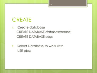
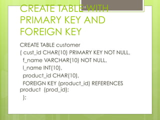
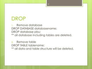
DROP
1. Remove database
DROPDATABASE databasename;
DROP database pbu;
** all database including tables are deleted.
2. Remove table
DROP TABLE tablename;
** all data and table structure will be deleted.
21
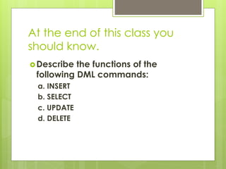
At the endof this class you
should know.
› Describe the functions of the
following DML commands:
a. INSERT
b. SELECT
c. UPDATE
d. DELETE
25.
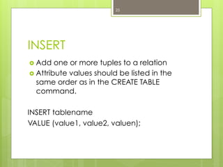
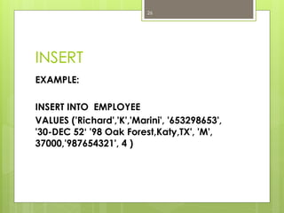
INSERT
› Add oneor more tuples to a relation
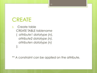
› Attribute values should be listed in the
same order as in the CREATE TABLE
command.
INSERT tablename
VALUE (value1, value2, valuen);
25
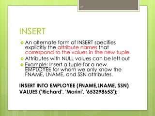
INSERT
› An alternateform of INSERT specifies
explicitly the attribute names that
correspond to the values in the new tuple.
› Attributes with NULL values can be left out
› Example: Insert a tuple for a new
EMPLOYEE for whom we only know the
FNAME, LNAME, and SSN attributes.
INSERT INTO EMPLOYEE (FNAME,LNAME, SSN)
VALUES ('Richard', 'Marini', '653298653');
27
28.
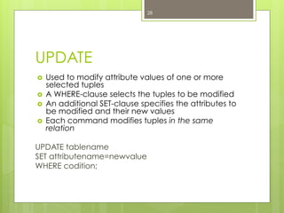
UPDATE
› Used tomodify attribute values of one or more
selected tuples
› A WHERE-clause selects the tuples to be modified
› An additional SET-clause specifies the attributes to
be modified and their new values
› Each command modifies tuples in the same
relation
UPDATE tablename
SET attributename=newvalue
WHERE codition;
28
29.
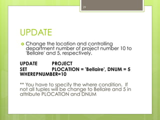
UPDATE
› Change thelocation and controlling
department number of project number 10 to
'Bellaire' and 5, respectively.
UPDATE PROJECT
SET PLOCATION = 'Bellaire', DNUM = 5
WHEREPNUMBER=10
** You have to specify the where condition. If
not all tuples will be change to Bellaire and 5 in
attribute PLOCATION and DNUM
29
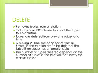
DELETE
› Removes tuplesfrom a relation
› Includes a WHERE-clause to select the tuples
to be deleted
› Tuples are deleted from only one table at a
time
› A missing WHERE-clause specifies that all
tuples in the relation are to be deleted; the
table then becomes an empty table
› The number of tuples deleted depends on the
number of tuples in the relation that satisfy the
WHERE-clause
31
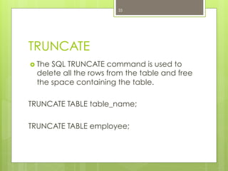
TRUNCATE
› The SQLTRUNCATE command is used to
delete all the rows from the table and free
the space containing the table.
TRUNCATE TABLE table_name;
TRUNCATE TABLE employee;
33
34.
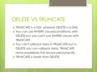
DELETE VS TRUNCATE
› TRUNCATE is a DDL whereas DELETE is a DML
› You can use WHERE clause(conditions) with
DELETE but you can't use WHERE clause with
TRUNCATE .
› You can't rollback data in TRUNCATE but in
DELETE you can rollback data. TRUNCATE
removes(delete) the record permanently.
› TRUNCATE is faster than DELETE.
34
36.
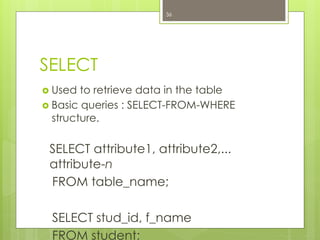
SELECT
› Used toretrieve data in the table
› Basic queries : SELECT-FROM-WHERE
structure.
SELECT attribute1, attribute2,...
attribute-n
FROM table_name;
SELECT stud_id, f_name
FROM student;
36
37.
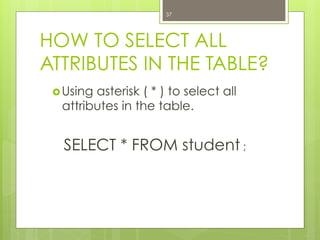
HOW TO SELECTALL
ATTRIBUTES IN THE TABLE?
› Using asterisk ( * ) to select all
attributes in the table.
SELECT * FROM student ;
37
38.
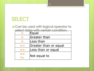
SELECT
› Can beused with logical operator to
select data with certain condition.
38
= Equal
> Greater than
< Less than
>= Greater than or equal
<= Less than or equal
<>
!=
Not equal to
39.
SELECT
39
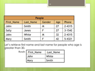
• People
• First_Name • Last_Name • Gender• Age • Phone
• John • Smith • M • 27 • 2-4315
• Sally • Jones • F • 27 • 3-1542
• John • White • M • 32 • 2-4315
• Mary • Smith • F • 42 • 5-4321
• First_Name • Last_Name
John White
Mary Smith
Result:
Let’s retrieve first name and last name for people who age is
greater than 30.
41.
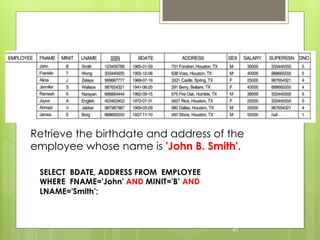
SELECT
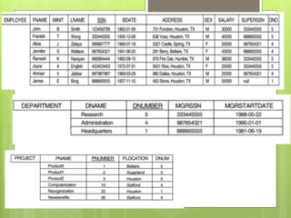
Retrieve the birthdateand address of the
employee whose name is 'John B. Smith'.
41
SELECT BDATE, ADDRESS FROM EMPLOYEE
WHERE FNAME='John' AND MINIT='B’ AND
LNAME='Smith’;
42.
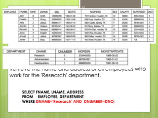
Retrieve the nameand address of all employees who
work for the 'Research' department.
42
SELECT FNAME, LNAME, ADDRESS
FROM EMPLOYEE, DEPARTMENT
WHERE DNAME='Research' AND DNUMBER=DNO;
43.
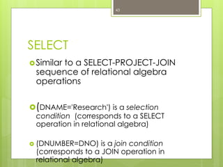
SELECT
› Similar to aSELECT-PROJECT-JOIN
sequence of relational algebra
operations
› (DNAME='Research') is a selection
condition (corresponds to a SELECT
operation in relational algebra)
› (DNUMBER=DNO) is a join condition
(corresponds to a JOIN operation in
relational algebra)
43
SELECT
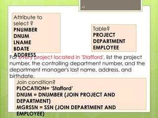
For every projectlocated in 'Stafford', list the project
number, the controlling department number, and the
department manager's last name, address, and
birthdate.
45
Attribute to
select ?
PNUMBER
DNUM
LNAME
BDATE
ADDRESS
Table?
PROJECT
DEPARTMENT
EMPLOYEE
Join condition?
PLOCATION= ‘Stafford’
DNUM = DNUMBER (JOIN PROJECT AND
DEPARTMENT)
MGRSSN = SSN (JOIN DEPARTMENT AND
EMPLOYEE)
46.
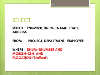
SELECT
SELECT PNUMBER, DNUM,LNAME, BDATE,
ADDRESS
FROM PROJECT, DEPARTMENT, EMPLOYEE
WHERE DNUM=DNUMBER AND
MGRSSN=SSN AND
PLOCATION='Stafford‘;
46
47.
SELECT
› There are twojoin conditions
› The join condition
DNUM=DNUMBER relates a
project to its controlling
department
› The join condition MGRSSN=SSN
relates the controlling
department to the employee
who manages that
47
48.
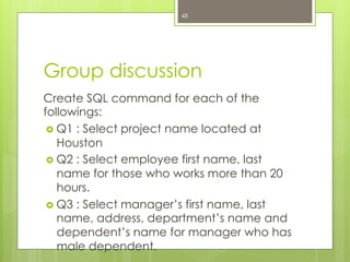
Group discussion
Create SQLcommand for each of the
followings:
› Q1 : Select project name located at
Houston
› Q2 : Select employee first name, last
name for those who works more than 20
hours.
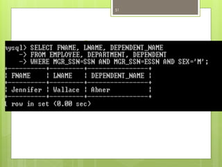
› Q3 : Select manager’s first name, last
name, address, department’s name and
dependent’s name for manager who has
male dependent.
48
At the endof this class you
should know.
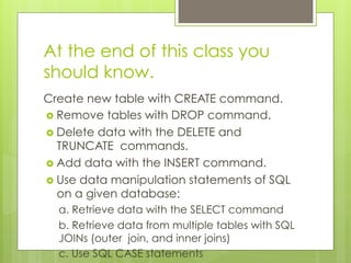
Create new table with CREATE command.
› Remove tables with DROP command.
› Delete data with the DELETE and
TRUNCATE commands.
› Add data with the INSERT command.
› Use data manipulation statements of SQL
on a given database:
a. Retrieve data with the SELECT command
b. Retrieve data from multiple tables with SQL
JOINs (outer join, and inner joins)
c. Use SQL CASE statements
54.
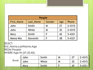
IN • People
• First_Name • Last_Name• Gender • Age • Phone
• John • Smith • M • 27 • 2-4315
• John • White • M • 32 • 2-4315
• Mary • Smith • F • 42 • 5-4321
• Mama Mia • Steventh • F • 38 • 5-4321
SELECT
First_Name,LastName,Age
FROM People
WHERE Age IN (27,32,42);
Result:
• John • Smith • M • 27 • 2-4315
• John • White • M • 32 • 2-4315
• Mary • Smith • F • 42 • 5-4321
55.
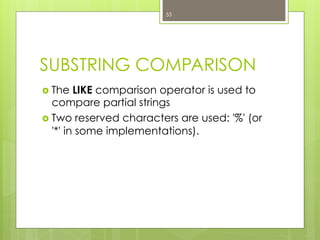
SUBSTRING COMPARISON
› TheLIKE comparison operator is used to
compare partial strings
› Two reserved characters are used: '%' (or
'*' in some implementations).
55
56.
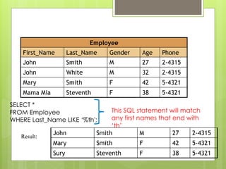
LIKE Employee
First_Name Last_NameGender Age Phone
John Smith M 27 2-4315
John White M 32 2-4315
Mary Smith F 42 5-4321
Mama Mia Steventh F 38 5-4321
John Smith M 27 2-4315
Mary Smith F 42 5-4321
Sury Steventh F 38 5-4321
SELECT *
FROM Employee
WHERE Last_Name LIKE ‘%th';
This SQL statement will match
any first names that end with
‘th’
Result:
57.
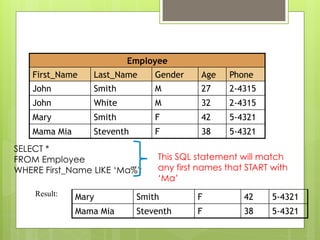
LIKE Employee
First_Name Last_NameGender Age Phone
John Smith M 27 2-4315
John White M 32 2-4315
Mary Smith F 42 5-4321
Mama Mia Steventh F 38 5-4321
SELECT *
FROM Employee
WHERE First_Name LIKE ‘Ma%';
This SQL statement will match
any first names that START with
‘Ma’
Mary Smith F 42 5-4321
Mama Mia Steventh F 38 5-4321
Result:
58.
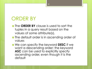
ORDER BY
› TheORDER BY clause is used to sort the
tuples in a query result based on the
values of some attribute(s).
› The default order is in ascending order of
values
› We can specify the keyword DESC if we
want a descending order; the keyword
ASC can be used to explicitly specify
ascending order, even though it is the
default
58
59.
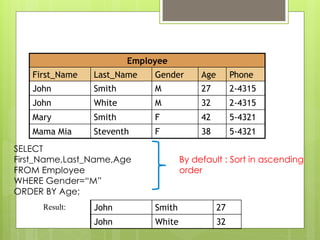
ORDER BYEmployee
First_Name Last_NameGender Age Phone
John Smith M 27 2-4315
John White M 32 2-4315
Mary Smith F 42 5-4321
Mama Mia Steventh F 38 5-4321
SELECT
First_Name,Last_Name,Age
FROM Employee
WHERE Gender=“M”
ORDER BY Age;
By default : Sort in ascending
order
Result: John Smith 27
John White 32
60.
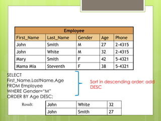
ORDER BYEmployee
First_Name Last_NameGender Age Phone
John Smith M 27 2-4315
John White M 32 2-4315
Mary Smith F 42 5-4321
Mama Mia Steventh F 38 5-4321
SELECT
First_Name,LastName,Age
FROM Employee
WHERE Gender=“M”
ORDER BY Age DESC;
Sort in descending order: add
DESC
Result: John White 32
John Smith 27
61.
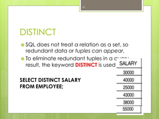
DISTINCT
› SQL doesnot treat a relation as a set, so
redundant data or tuples can appear.
› To eliminate redundant tuples in a query
result, the keyword DISTINCT is used
SELECT DISTINCT SALARY
FROM EMPLOYEE;
61
62.
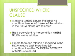
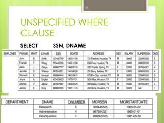
UNSPECIFIED WHERE
CLAUSE
› Amissing WHERE-clause indicates no
condition; hence, all tuples of the relation
in the FROM-clause are selected
› This is equivalent to the condition WHERE
TRUE is in one relation.
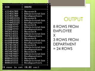
› If more than one relation is specified in the
FROM-clause and there is no join
condition, then the CARTESIAN PRODUCT
of tuples is selected
62
UNSPECIFIED WHERE
CLAUSE
› The SQLbefore produced a large
relation which concatenate with
every tuples from both relations
› It is extremely important not to
overlook specifying any selection
and join conditions in the WHERE-
clause; otherwise, incorrect and
very large relations may result
65
66.
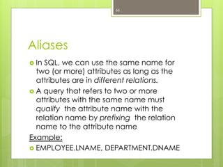
Aliases
› In SQL,we can use the same name for
two (or more) attributes as long as the
attributes are in different relations.
› A query that refers to two or more
attributes with the same name must
qualify the attribute name with the
relation name by prefixing the relation
name to the attribute name
Example:
› EMPLOYEE.LNAME, DEPARTMENT.DNAME
66
67.
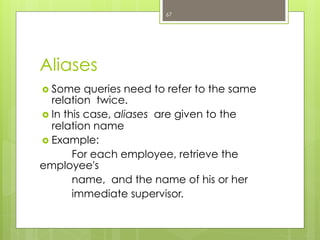
Aliases
› Some queriesneed to refer to the same
relation twice.
› In this case, aliases are given to the
relation name
› Example:
For each employee, retrieve the
employee's
name, and the name of his or her
immediate supervisor.
67
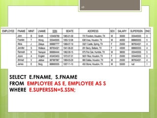
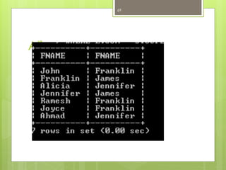
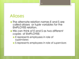
Aliases
› The alternaterelation names E and S are
called aliases or tuple variables for the
EMPLOYEE relation.
› We can think of E and S as two different
copies of EMPLOYEE;
› E represents employees in role of
supervisees
› S represents employees in role of supervisors
70
71.
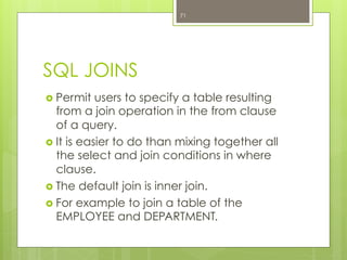
SQL JOINS
› Permitusers to specify a table resulting
from a join operation in the from clause
of a query.
› It is easier to do than mixing together all
the select and join conditions in where
clause.
› The default join is inner join.
› For example to join a table of the
EMPLOYEE and DEPARTMENT.
71
72.
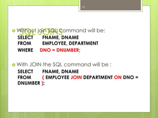
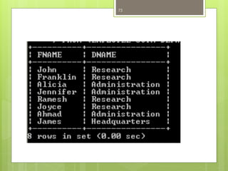
SQL JOINS› Withoutjoin SQL command will be:
SELECT FNAME, DNAME
FROM EMPLOYEE, DEPARTMENT
WHERE DNO = DNUMBER;
› With JOIN the SQL command will be :
SELECT FNAME, DNAME
FROM ( EMPLOYEE JOIN DEPARTMENT ON DNO =
DNUMBER );
72
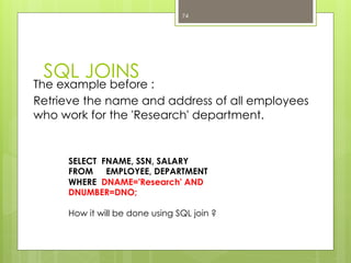
SQL JOINS
The examplebefore :
Retrieve the name and address of all employees
who work for the 'Research' department.
74
SELECT FNAME, SSN, SALARY
FROM EMPLOYEE, DEPARTMENT
WHERE DNAME='Research' AND
DNUMBER=DNO;
How it will be done using SQL join ?
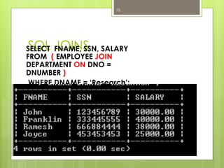
75.
SQL JOINSSELECT FNAME,SSN, SALARY
FROM ( EMPLOYEE JOIN
DEPARTMENT ON DNO =
DNUMBER )
WHERE DNAME = ‘Research’;
75
76.
SQL JOINS
SELECT PNUMBER,PNAME, DNUM, FNAME, SSN,
SALARY
FROM PROJECT, DEPARTMENT, EMPLOYEE
WHERE DNUM=DNUMBER AND
MGRSSN=SSN AND
PLOCATION='Stafford‘;
How it will be done with SQL Join ?
76
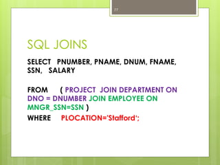
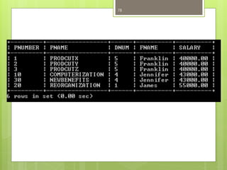
77.
SQL JOINS
SELECT PNUMBER,PNAME, DNUM, FNAME,
SSN, SALARY
FROM ( PROJECT JOIN DEPARTMENT ON
DNO = DNUMBER JOIN EMPLOYEE ON
MNGR_SSN=SSN )
WHERE PLOCATION='Stafford‘;
77
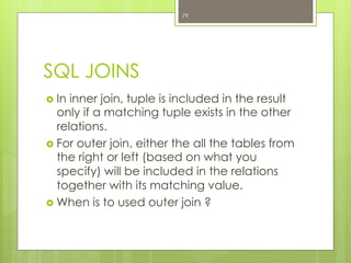
SQL JOINS
› Ininner join, tuple is included in the result
only if a matching tuple exists in the other
relations.
› For outer join, either the all the tables from
the right or left (based on what you
specify) will be included in the relations
together with its matching value.
› When is to used outer join ?
79
80.
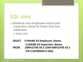
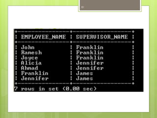
SQL Joins
› Retrieveonly employee name and
supervisor name for those who has
supervisor.
› Inner Join
SELECT E.FNAME AS Employee_Name,
S.LNAME AS Supervisor_Name
FROM (EMPLOYEE AS E JOIN EMPLOYEE AS S
ON E.SUPERSSN=S.SSN)
80
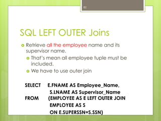
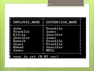
SQL LEFT OUTERJoins
› Retrieve all the employee name and its
supervisor name.
› That’s mean all employee tuple must be
included.
› We have to use outer join
SELECT E.FNAME AS Employee_Name,
S.LNAME AS Supervisor_Name
FROM (EMPLOYEE AS E LEFT OUTER JOIN
EMPLOYEE AS S
ON E.SUPERSSN=S.SSN)
82
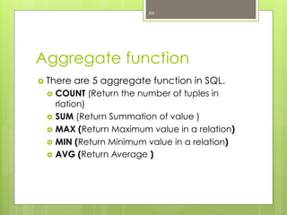
Aggregate function
› Thereare 5 aggregate function in SQL.
› COUNT (Return the number of tuples in
rlation)
› SUM (Return Summation of value )
› MAX (Return Maximum value in a relation)
› MIN (Return Minimum value in a relation)
› AVG (Return Average )
84
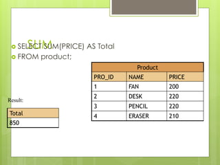
SUM› SELECT SUM(PRICE)AS Total
› FROM product;
Result:
Total
850
Product
PRO_ID NAME PRICE
1 FAN 200
2 DESK 220
3 PENCIL 220
4 ERASER 210
87.
AVG› SELECT AVG(PRICE)AS total
› FROM product;
Result:
total
212.5
Product
PRO_ID NAME PRICE
1 FAN 200
2 DESK 220
3 PENCIL 220
4 ERASER 210
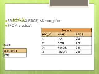
88.
MAX› SELECT MAX(PRICE)AS max_price
› FROM product;
Result:
max_price
220
Product
PRO_ID NAME PRICE
1 FAN 200
2 DESK 220
3 PENCIL 220
4 ERASER 210
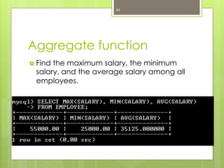
89.
Aggregate function
› Findthe maximum salary, the minimum
salary, and the average salary among all
employees.
› SELECT MAX(SALARY), MIN(SALARY),
AVG(SALARY)
FROM EMPLOYEE;
89
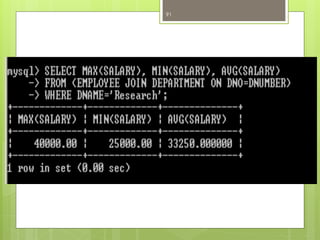
90.
GROUP DISCUSSION
QUESTION1
Find themaximum salary, the minimum salary,
and the average salary among employees who
work for the 'Research' department.
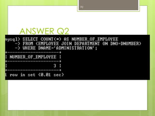
QUESTION2
Retrieve the number of employees in the
‘Administration Department' department
90
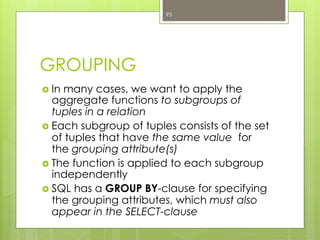
GROUPING
› In manycases, we want to apply the
aggregate functions to subgroups of
tuples in a relation
› Each subgroup of tuples consists of the set
of tuples that have the same value for
the grouping attribute(s)
› The function is applied to each subgroup
independently
› SQL has a GROUP BY-clause for specifying
the grouping attributes, which must also
appear in the SELECT-clause
93
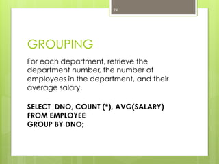
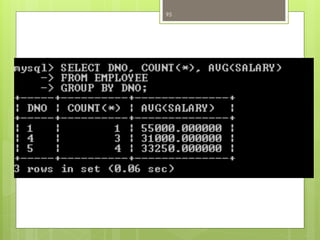
94.
GROUPING
For each department,retrieve the
department number, the number of
employees in the department, and their
average salary.
SELECT DNO, COUNT (*), AVG(SALARY)
FROM EMPLOYEE
GROUP BY DNO;
94
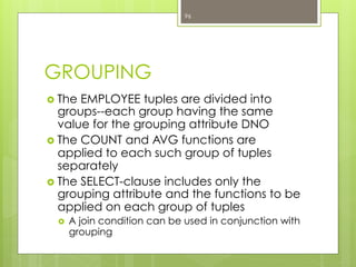
GROUPING
› The EMPLOYEEtuples are divided into
groups--each group having the same
value for the grouping attribute DNO
› The COUNT and AVG functions are
applied to each such group of tuples
separately
› The SELECT-clause includes only the
grouping attribute and the functions to be
applied on each group of tuples
› A join condition can be used in conjunction with
grouping
96
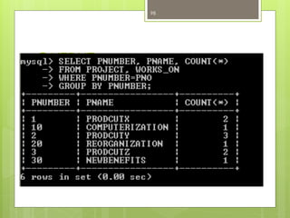
97.
GROUPING
› For eachproject, retrieve the project
number, project name, and the number
of employees who work on that project.
SELECT PNUMBER, PNAME, COUNT (*)
FROM PROJECT, WORKS_ON
WHERE PNUMBER=PNO
GROUP BY PNUMBER;
› In this case, the grouping and functions are
applied after the joining of the two relations
97
THE HAVING-CLAUSE
› Sometimeswe want to retrieve the values
of these functions for only those groups
that satisfy certain conditions.
› The HAVING-clause is used for specifying a
selection condition on groups (rather than
on individual tuples)
99
100.
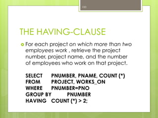
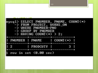
THE HAVING-CLAUSE
› Foreach project on which more than two
employees work , retrieve the project
number, project name, and the number
of employees who work on that project.
SELECT PNUMBER, PNAME, COUNT (*)
FROM PROJECT, WORKS_ON
WHERE PNUMBER=PNO
GROUP BY PNUMBER
HAVING COUNT (*) > 2;
100
Summary of SQLQueries
› A query in SQL can consist of up to six
clauses, but only the first two, SELECT and
FROM, are mandatory. The clauses are
specified in the following order:
SELECT <attribute list>
FROM <table list>
[WHERE <condition>]
[GROUP BY <grouping attribute(s)>]
[HAVING <group condition>]
[ORDER BY <attribute list>]
102
103.
Summary of SQLQueries
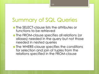
› The SELECT-clause lists the attributes or
functions to be retrieved
› The FROM-clause specifies all relations (or
aliases) needed in the query but not those
needed in nested queries
› The WHERE-clause specifies the conditions
for selection and join of tuples from the
relations specified in the FROM-clause
103
104.
Summary of SQLQueries
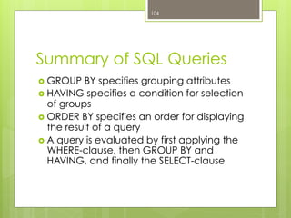
› GROUP BY specifies grouping attributes
› HAVING specifies a condition for selection
of groups
› ORDER BY specifies an order for displaying
the result of a query
› A query is evaluated by first applying the
WHERE-clause, then GROUP BY and
HAVING, and finally the SELECT-clause
104
105.
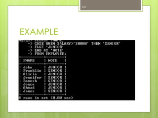
SQL CASE
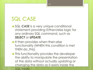
› SQLCASE is a very unique conditional
statement providing if/then/else logic for
any ordinary SQL command, such as
SELECT or UPDATE.
› It then provides when-then-else
functionality (WHEN this condition is met
THEN do_this).
› This functionality provides the developer
the ability to manipulate the presentation
of the data without actually updating or
changing the data as it exists inside the
SQL table.
105
106.
SQL CASE
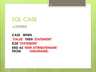
› SYNTAX
CASEWHEN
‘VALUE’ THEN ‘STATEMENT’
ELSE ‘STATEMENT’
END AS ‘NEW ATTRIBUTENAME’
FROM TABLENAME;
106


![Summary of SQL Queries
› A query in SQL can consist of up to six
clauses, but only the first two, SELECT and
FROM, are mandatory. The clauses are
specified in the following order:
SELECT <attribute list>
FROM <table list>
[WHERE <condition>]
[GROUP BY <grouping attribute(s)>]
[HAVING <group condition>]
[ORDER BY <attribute list>]
102](https://image.slidesharecdn.com/chapter4-structuredquerylanguage-150826165241-lva1-app6891/85/Chapter-4-Structured-Query-Language-102-320.jpg)