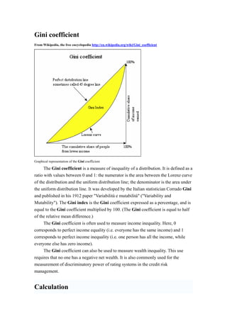
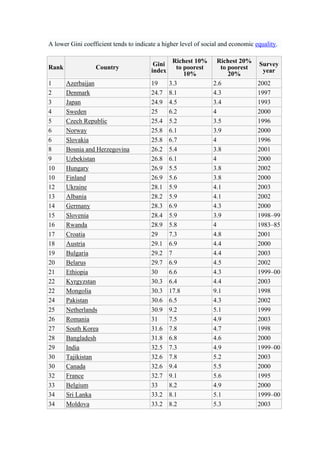
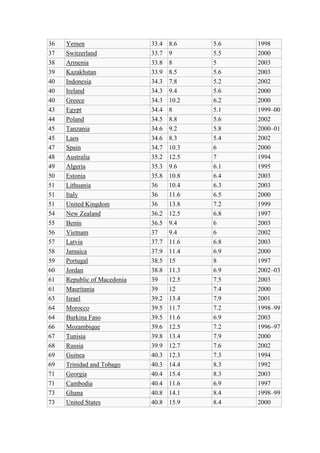
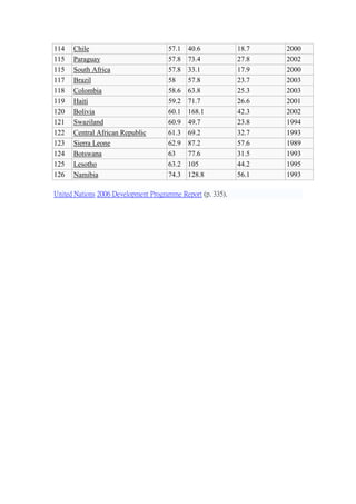
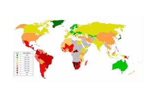
The document defines and explains the Gini coefficient, a measure of statistical dispersion used as a gauge of economic inequality. It is a ratio with a value between 0 and 1, with 0 representing perfect equality and 1 representing perfect inequality. The Gini coefficient is calculated based on the Lorenz curve, which plots cumulative incomes against the percentage of the population. The document provides various methods for calculating the Gini coefficient and discusses its advantages and limitations as a measure of inequality. It also includes a table ranking countries by their Gini coefficients.

1. Gini coefficient
From Wikipedia, the free encyclopedia http://en.wikipedia.org/wiki/Gini_coefficient
Graphical representation of the Gini coefficient
The Gini coefficient is a measure of inequality of a distribution. It is defined as a
ratio with values between 0 and 1: the numerator is the area between the Lorenz curve
of the distribution and the uniform distribution line; the denominator is the area under
the uniform distribution line. It was developed by the Italian statistician Corrado Gini
and published in his 1912 paper "Variabilità e mutabilità" ("Variability and
Mutability"). The Gini index is the Gini coefficient expressed as a percentage, and is
equal to the Gini coefficient multiplied by 100. (The Gini coefficient is equal to half
of the relative mean difference.)
The Gini coefficient is often used to measure income inequality. Here, 0
corresponds to perfect income equality (i.e. everyone has the same income) and 1
corresponds to perfect income inequality (i.e. one person has all the income, while
everyone else has zero income).
The Gini coefficient can also be used to measure wealth inequality. This use
requires that no one has a negative net wealth. It is also commonly used for the
measurement of discriminatory power of rating systems in the credit risk
management.
Calculation

2. The Gini coefficient is defined as a ratio of the areas on the Lorenz curve
diagram. If the area between the line of perfect equality and Lorenz curve is A, and
the area under the Lorenz curve is B, then the Gini coefficient is A/(A+B). Since A+B
= 0.5, the Gini coefficient, G = 2A = 1-2B. If the Lorenz curve is represented by the
function Y = L(X), the value of B can be found with integration and:
In some cases, this equation can be applied to calculate the Gini coefficient
without direct reference to the Lorenz curve. For example:
• For a population with values yi, i = 1 to n, that are indexed in non-decreasing
order ( yi ≤ yi+1):
• For a discrete probability function f(y), where yi, i = 1 to n, are the points with
nonzero probabilities and which are indexed in increasing order ( yi < yi+1):
where:
and
• For a cumulative distribution function F(y) that is piecewise differentiable, has
a mean μ, and is zero for all negative values of y:
Since the Gini coefficient is half the relative mean difference, it can also be
calculated using formulas for the relative mean difference.
For a random sample S consisting of values yi, i = 1 to n, that are indexed in
non-decreasing order ( yi ≤ yi+1), the statistic:

3. is a consistent estimator of the population Gini coefficient, but is not, in general,
unbiased. Like the relative mean difference, there does not exist a sample statistic that
is in general an unbiased estimator of the population Gini coefficient. Confidence
intervals for the population Gini coefficient can be calculated using bootstrap
techniques.
Sometimes the entire Lorenz curve is not known, and only values at certain
intervals are given. In that case, the Gini coefficient can be approximated by using
various techniques for interpolating the missing values of the Lorenz curve. If ( X k ,
Yk ) are the known points on the Lorenz curve, with the X k indexed in increasing
order ( X k - 1 < X k ), so that:
• Xk is the cumulated proportion of the population variable, for k = 0,...,n, with
X0 = 0, Xn = 1.
• Yk is the cumulated proportion of the income variable, for k = 0,...,n, with Y0
= 0, Yn = 1.
If the Lorenz curve is approximated on each interval as a line between consecutive
points, then the area B can be approximated with trapezoids and:
is the resulting approximation for G. More accurate results can be obtained using
other methods to approximate the area B, such as approximating the Lorenz curve
with a quadratic function across pairs of intervals, or building an appropriately
smooth approximation to the underlying distribution function that matches the known
data. If the population mean and boundary values for each interval are also known,
these can also often be used to improve the accuracy of the approximation.

4. While most developed European nations tend to have Gini coefficients between
0.24 and 0.36, the United States Gini coefficient is above 0.4, indicating that the
United States has greater inequality. Using the Gini can help quantify differences in
welfare and compensation policies and philosophies. However it should be borne in
mind that the Gini coefficient can be misleading when used to make political
comparisons between large and small countries (see criticisms section).
Correlation with per-capita GDP
Poor countries (those with low per-capita GDP) have Gini coefficients that fall
over the whole range from low (0.25) to high (0.71), while rich countries have
generally low Gini coefficient (under 0.40).
Advantages as a measure of inequality
• The Gini coefficient's main advantage is that it is a measure of inequality by
means of a ratio analysis, rather than a variable unrepresentative of most of the
population, such as per capita income or gross domestic product.
• It can be used to compare income distributions across different population
sectors as well as countries, for example the Gini coefficient for urban areas
differs from that of rural areas in many countries (though the United States'
urban and rural Gini coefficients are nearly identical).
• It is sufficiently simple that it can be compared across countries and be easily
interpreted. GDP statistics are often criticised as they do not represent changes
for the whole population; the Gini coefficient demonstrates how income has
changed for poor and rich. If the Gini coefficient is rising as well as GDP,
poverty may not be improving for the majority of the population.
• The Gini coefficient can be used to indicate how the distribution of income
has changed within a country over a period of time, thus it is possible to see if
inequality is increasing or decreasing.
• The Gini coefficient satisfies four important principles:
o Anonymity: it does not matter who the high and low earners are.

5. o Scale independence: the Gini coefficient does not consider the size of
the economy, the way it is measured, or whether it is a rich or poor
country on average.
o Population independence: it does not matter how large the population
of the country is.
o Transfer principle: if income (less than the difference), is transferred
from a rich person to a poor person the resulting distribution is more
equal.
Disadvantages as a measure of inequality
• The Gini coefficient measured for a large economically diverse country will
generally result in a much higher coefficient than each of its regions has
individually. For this reason the scores calculated for individual countries
within the EU are difficult to compare with the score of the entire US.
• Comparing income distributions among countries may be difficult because
benefits systems may differ. For example, some countries give benefits in the
form of money while others give food stamps, which may not be counted as
income in the Lorenz curve and therefore not taken into account in the Gini
coefficient.
• The measure will give different results when applied to individuals instead of
households. When different populations are not measured with consistent
definitions, comparison is not meaningful.
• The Lorenz curve may understate the actual amount of inequality if richer
households are able to use income more efficiently than lower income
households. From another point of view, measured inequality may be the
result of more or less efficient use of household incomes.
• As for all statistics, there will be systematic and random errors in the data. The
meaning of the Gini coefficient decreases as the data become less accurate.
Also, countries may collect data differently, making it difficult to compare
statistics between countries.
• Economies with similar incomes and Gini coefficients can still have very
different income distributions. This is because the Lorenz curves can have
different shapes and yet still yield the same Gini coefficient. As an extreme

6. example, an economy where half the households have no income, and the
other half share income equally has a Gini coefficient of ½; but an economy
with complete income equality, except for one wealthy household that has half
the total income, also has a Gini coefficient of ½.
• Too often only the Gini coefficient is quoted without describing the
proportions of the quantiles used for measurement. As with other inequality
coefficients, the Gini coefficient is influenced by the granularity of the
measurements. For example, five 20% quantiles (low granularity) will yield a
lower Gini coefficient than twenty 5% quantiles (high granularity) taken from
the same distribution.
As one result of this criticism, additionally to or in competition with the Gini
coefficient entropy measures are frequently used (e.g. the Atkinson and Theil indices).
These measures attempt to compare the distribution of resources by intelligent players
in the market with a maximum entropy random distribution, which would occur if
these players acted like non-intelligent particles in a closed system following the laws
of statistical physics.

7. A lower Gini coefficient tends to indicate a higher level of social and economic equality.
Rank Country Gini
index
Richest 10%
to poorest
10%
Richest 20%
to poorest
20%
Survey
year
1 Azerbaijan 19 3.3 2.6 2002
2 Denmark 24.7 8.1 4.3 1997
3 Japan 24.9 4.5 3.4 1993
4 Sweden 25 6.2 4 2000
5 Czech Republic 25.4 5.2 3.5 1996
6 Norway 25.8 6.1 3.9 2000
6 Slovakia 25.8 6.7 4 1996
8 Bosnia and Herzegovina 26.2 5.4 3.8 2001
9 Uzbekistan 26.8 6.1 4 2000
10 Hungary 26.9 5.5 3.8 2002
10 Finland 26.9 5.6 3.8 2000
12 Ukraine 28.1 5.9 4.1 2003
13 Albania 28.2 5.9 4.1 2002
14 Germany 28.3 6.9 4.3 2000
15 Slovenia 28.4 5.9 3.9 1998–99
16 Rwanda 28.9 5.8 4 1983–85
17 Croatia 29 7.3 4.8 2001
18 Austria 29.1 6.9 4.4 2000
19 Bulgaria 29.2 7 4.4 2003
20 Belarus 29.7 6.9 4.5 2002
21 Ethiopia 30 6.6 4.3 1999–00
22 Kyrgyzstan 30.3 6.4 4.4 2003
22 Mongolia 30.3 17.8 9.1 1998
24 Pakistan 30.6 6.5 4.3 2002
25 Netherlands 30.9 9.2 5.1 1999
26 Romania 31 7.5 4.9 2003
27 South Korea 31.6 7.8 4.7 1998
28 Bangladesh 31.8 6.8 4.6 2000
29 India 32.5 7.3 4.9 1999–00
30 Tajikistan 32.6 7.8 5.2 2003
30 Canada 32.6 9.4 5.5 2000
32 France 32.7 9.1 5.6 1995
33 Belgium 33 8.2 4.9 2000
34 Sri Lanka 33.2 8.1 5.1 1999–00
34 Moldova 33.2 8.2 5.3 2003

8. 36 Yemen 33.4 8.6 5.6 1998
37 Switzerland 33.7 9 5.5 2000
38 Armenia 33.8 8 5 2003
39 Kazakhstan 33.9 8.5 5.6 2003
40 Indonesia 34.3 7.8 5.2 2002
40 Ireland 34.3 9.4 5.6 2000
40 Greece 34.3 10.2 6.2 2000
43 Egypt 34.4 8 5.1 1999–00
44 Poland 34.5 8.8 5.6 2002
45 Tanzania 34.6 9.2 5.8 2000–01
45 Laos 34.6 8.3 5.4 2002
47 Spain 34.7 10.3 6 2000
48 Australia 35.2 12.5 7 1994
49 Algeria 35.3 9.6 6.1 1995
50 Estonia 35.8 10.8 6.4 2003
51 Lithuania 36 10.4 6.3 2003
51 Italy 36 11.6 6.5 2000
51 United Kingdom 36 13.8 7.2 1999
54 New Zealand 36.2 12.5 6.8 1997
55 Benin 36.5 9.4 6 2003
56 Vietnam 37 9.4 6 2002
57 Latvia 37.7 11.6 6.8 2003
58 Jamaica 37.9 11.4 6.9 2000
59 Portugal 38.5 15 8 1997
60 Jordan 38.8 11.3 6.9 2002–03
61 Republic of Macedonia 39 12.5 7.5 2003
61 Mauritania 39 12 7.4 2000
63 Israel 39.2 13.4 7.9 2001
64 Morocco 39.5 11.7 7.2 1998–99
64 Burkina Faso 39.5 11.6 6.9 2003
66 Mozambique 39.6 12.5 7.2 1996–97
67 Tunisia 39.8 13.4 7.9 2000
68 Russia 39.9 12.7 7.6 2002
69 Guinea 40.3 12.3 7.3 1994
69 Trinidad and Tobago 40.3 14.4 8.3 1992
71 Georgia 40.4 15.4 8.3 2003
71 Cambodia 40.4 11.6 6.9 1997
73 Ghana 40.8 14.1 8.4 1998–99
73 United States 40.8 15.9 8.4 2000

9. 73 Turkmenistan 40.8 12.3 7.7 1998
76 Senegal 41.3 12.8 7.5 1995
77 Thailand 42 12.6 7.7 2002
78 Zambia 42.1 13.9 8 2002–03
79 Burundi 42.4 19.3 9.5 1998
80 Singapore 42.5 17.7 9.7 1998
80 Kenya 42.5 13.6 8.2 1997
82 Uganda 43 14.9 8.4 1999
82 Iran 43 17.2 9.7 1998
84 Nicaragua 43.1 15.5 8.8 2001
85 Hong Kong, China (SAR) 43.4 17.8 9.7 1996
86 Turkey 43.6 16.8 9.3 2003
87 Nigeria 43.7 17.8 9.7 2003
87 Ecuador 43.7 44.9 17.3 1998
89 Venezuela 44.1 20.4 10.6 2000
90 Côte d’Ivoire 44.6 16.6 9.7 2002
90 Cameroon 44.6 15.7 9.1 2001
92 People's Republic of China 44.7 18.4 10.7 2001
93 Uruguay 44.9 17.9 10.2 2003
94 Philippines 46.1 16.5 9.7 2000
95 Guinea-Bissau 47 19 10.3 1993
96 Nepal 47.2 15.8 9.1 2003–04
97 Madagascar 47.5 19.2 11 2001
98 Malaysia 49.2 22.1 12.4 1997
99 Mexico 49.5 24.6 12.8 2002
100 Costa Rica 49.9 30 14.2 2001
101 Zimbabwe 50.1 22 12 1995
102 Gambia 50.2 20.2 11.2 1998
103 Malawi 50.3 22.7 11.6 1997
104 Niger 50.5 46 20.7 1995
104 Mali 50.5 23.1 12.2 1994
106 Papua New Guinea 50.9 23.8 12.6 1996
107 Dominican Republic 51.7 30 14.4 2003
108 El Salvador 52.4 57.5 20.9 2002
109 Argentina 52.8 34.5 17.6 2003
110 Honduras 53.8 34.2 17.2 2003
111 Peru 54.6 40.5 18.6 2002
112 Guatemala 55.1 48.2 20.3 2002
113 Panama 56.4 54.7 23.9 2002

10. 114 Chile 57.1 40.6 18.7 2000
115 Paraguay 57.8 73.4 27.8 2002
115 South Africa 57.8 33.1 17.9 2000
117 Brazil 58 57.8 23.7 2003
118 Colombia 58.6 63.8 25.3 2003
119 Haiti 59.2 71.7 26.6 2001
120 Bolivia 60.1 168.1 42.3 2002
121 Swaziland 60.9 49.7 23.8 1994
122 Central African Republic 61.3 69.2 32.7 1993
123 Sierra Leone 62.9 87.2 57.6 1989
124 Botswana 63 77.6 31.5 1993
125 Lesotho 63.2 105 44.2 1995
126 Namibia 74.3 128.8 56.1 1993
United Nations 2006 Development Programme Report (p. 335).

12. year
China’s Gini
Coefficient
1991 0.38
1992 0.4
1993 0.4
1994 0.41
1995 0.41
1996 0.41
1997 0.41
1998 0.41
1999 0.42
2000 0.46
2001 0.45
2002 0.447
2003 0.447
2004 0.447
Source: Ravallion and Chen, 2004. China Statistical Yearbook (State Statistical
Bureau, 1992 1996 and 1997 2001).
http://www3.nccu.edu.tw/~jthuang/inequality.pdf

13. Gini Coefficient for China’s Income Distribution, 1981-2003
Source: Ravallion and Chen, Measuring Pro-Poor Growth, World Bank Policy Research Working
Paper 2666. August, 2001; The World Bank: Biannual on China’s Economy. Business Weekly: No.
9, 2004
http://www.cdrf.org.cn/2006cdf/news_Harmony.htm