Download to read offline


![Basic Multiplier Y = C + I + G Y = (a + bY) + I + G Y (1 – b) = a + I + G Y = (a + I + G) [1/(1 – b)] Since, b = MPC Y = (a + I + G) [1/(1 – MPC)] or Y = (a + I + G) [1/MPS]](https://image.slidesharecdn.com/chap11-110119223002-phpapp01/85/Chap11-5-320.jpg)
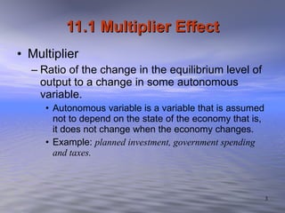
![Planned Investment Multiplier Y = C + I + G Y = [a + bY] + I + G Y = [a + b(Y- T)] + I + G Y = a + bY – bT + I + G Y (1 – b) = a – bT + I + G Y = (a – bT + I + G) [1/(1 – b)] --- Equation 11.1 ∆ Y/ ∆I = 1/(1 – b)](https://image.slidesharecdn.com/chap11-110119223002-phpapp01/85/Chap11-7-320.jpg)
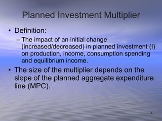
![If planned investment (I) increase by the amount of ∆I, income (Y) will increase by: ∆ Y = ∆I X [1/(1 – b)] Since b = MPC, and MPS = 1 – MPC, the expression become: ∆ Y = ∆I X [1/(1 – MPC)] ∆ Y = ∆I X [1/MPS] Therefore, the multiplier for planned investment is ????](https://image.slidesharecdn.com/chap11-110119223002-phpapp01/85/Chap11-8-320.jpg)
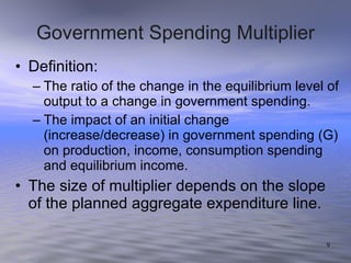
![From Equation 11.1: If government spending increase by the amount of ∆G, income (Y) will increase by: ∆ Y = ∆G X [1/(1 – b)] Since b = MPC, and MPS = 1 – MPC, the expression become: ∆ Y = ∆G X [1/(1 – MPC)] ∆ Y = ∆G X [1/MPS] Thus, the multiplier for government spending is ????](https://image.slidesharecdn.com/chap11-110119223002-phpapp01/85/Chap11-10-320.jpg)
![Figure: Government Spending Multiplier Example: ∆ Y = ∆G X [multiplier] = ∆G X [1/(1 – MPC)] = 50 X [1/(1 – 0.75)] = 50 X [4] ∆ Y = RM200 billion](https://image.slidesharecdn.com/chap11-110119223002-phpapp01/85/Chap11-11-320.jpg)
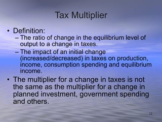
![Y = C + I + G Y = [a + bY] + I + G Y = [a + b(Y- T)] + I + G Y = a + bY – bT + I + G Y (1 – b) = a – bT + I + G Y = (a – bT + I + G) [1/(1 – b)] ∆ Y/ ∆T= -b/(1 – b) Tax Multiplier](https://image.slidesharecdn.com/chap11-110119223002-phpapp01/85/Chap11-13-320.jpg)
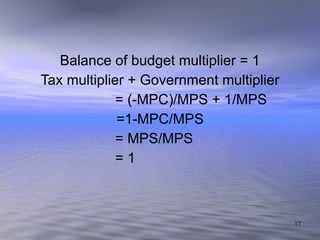
![If taxes increase by the amount of ∆T, income will increase by: ∆ Y = (-b) (∆T) X [1/(1 – b)] ∆ Y = (∆T) X [-b/(1 – b)] Since b = MPC, and MPS = 1 – MPC, the expression become: ∆ Y = ∆T X [-MPC/(1 – MPC)] ∆ Y = ∆T X [-(MPC/MPS)] Therefore, the multiplier for taxes are: -MPC/(1 – MPC) or -MPC/MPS](https://image.slidesharecdn.com/chap11-110119223002-phpapp01/85/Chap11-14-320.jpg)
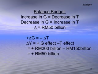
![Taxes (T) : In an economy with a MPC of 0.75, a RM50 billion of tax cuts magnifies the aggregate expenditure three times higher through the multiplier effect. ∆ Y = ∆T X [multiplier] = ∆T X [-MPC/(1 – MPC)] = 50 X [-0.75/(1 – 0.75)] = 50 X [-3] ∆ Y = - RM150 billion Example](https://image.slidesharecdn.com/chap11-110119223002-phpapp01/85/Chap11-15-320.jpg)
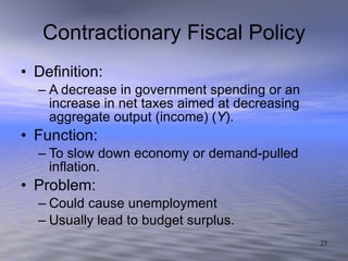
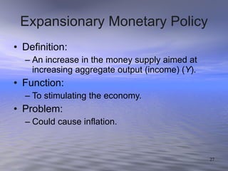
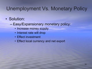
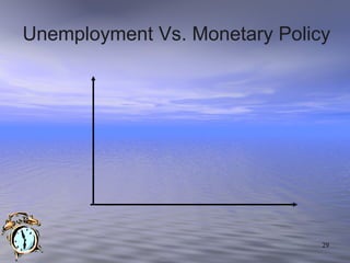
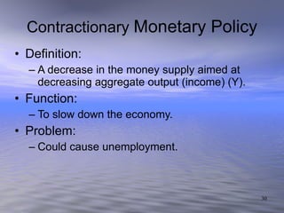
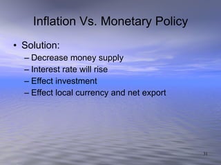
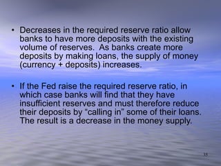


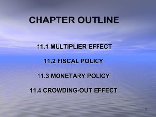
This chapter discusses fiscal and monetary policy. It defines the multiplier effect as the ratio of change in output to a change in autonomous spending. An expansionary fiscal policy increases government spending or cuts taxes to boost output, while a contractionary policy decreases spending or raises taxes. Monetary policy involves changing interest rates and the money supply via tools like open market operations. Both expansionary and contractionary monetary policies aim to respectively increase or decrease output. The crowding-out effect refers to how increased government spending may raise interest rates and reduce private investment.


