SlideShare a Scribd company logo
1
Ch 2 – Prob Solving by searching
To build a goal-based agent we need to answer the
following questions:
– What is the goal to be achieved?
– What are the actions?
– What relevant information is necessary to encode in
order to describe the state of the world, describe the
available transitions, and solve the problem?
Initial
state
Goal
state
Actions
2
What is the goal to be achieved?
 Could describe a situation we want to achieve, a
set of properties that we want to hold, etc.
 Requires defining a “goal test” so that we know
what it means to have achieved/satisfied our
goal.
3
What are the actions?
 Characterize the primitive actions or events that are
available for making changes in the world in order to
achieve a goal.
 Deterministic world: no uncertainty in an action’s
effects. Given an action (a.k.a. operator or move) and
a description of the current world state, the action
completely specifies
– whether that action can be applied to the current world
(i.e., is it applicable and legal), and
– what the exact state of the world will be after the action
is performed in the current world (i.e., no need for
“history” information to compute the new world).
4
Representing actions
Note also that actions in this framework can all
be considered as discrete events that occur at
an instant of time.
–For example, if “Sita is in class” and then
performs the action “go home,” then in the
next situation she is “at home.” There is no
representation of a point in time where she is
neither in class nor at home (i.e., in the state
of “going home”).
5
Representing actions
The number of actions / operators depends on the
representation used in describing a state.
– In the 8-puzzle, we could specify 4 possible moves for
each of the 8 tiles, resulting in a total of 4*8=32
operators.
– On the other hand, we could specify four moves for the
“blank” square and we would only need 4 operators.
Representational shift can greatly simplify a problem!
6
Representing states
 What information is necessary to encode about the world
to sufficiently describe all relevant aspects in solving the
goal? That is, what knowledge needs to be represented in
a state description to adequately describe the current state
or situation of the world?
 The size of a problem is usually described in terms of
the number of states that are possible.
– Tic-Tac-Toe has about 39 states.
– Checkers has about 1040 states.
– Rubik’s Cube has about 1019 states.
– Chess has about 10120 states in a typical game.
7
Defining a Problem as a State Space
1. Define a state space that contains all the possible
configurations of the relevant objects.
2. Specify one (or more) state(s) as the initial state(s).
3. Specify one (or more) state(s) as the goal state(s).
4. Specify a set of rules that describe available
actions (operators), considering:
 What assumptions are present in the informal
problem description?
 How general should the rules be?
 How much of work required to solve the problem
should be precompiled and represented in the rules?
8
2.2.1 Production Systems
 A set of rules (Knowledge Base) :
– LHS  RHS (if-part  then-part)
– Pattern  Action
– Antecedent  Consequent
 Knowledge containing information (temporary
or permanent) required to solve the current
task. (Working Memory)
 A control strategy to specify the order of testing
patterns and resolving possible conflicts
(Inference Engine)
 A rule applier.
9
Production System Major
Components
knowledge base
– contains essential information about the
problem domain
– often represented as facts and rules
inference engine
– mechanism to derive new knowledge from
the knowledge base and the information
provided by the user
– often based on the use of rules
10
Production (Rule-Based) System
Knowledge Base
Inference Engine
Working Memory
User
Interface
Agenda
11
Rule-Based System
 knowledge is encoded as IF … THEN rules
– these rules can also be written as production rules
 the inference engine determines which rule
antecedents are satisfied
– the left-hand side must “match” a fact in the working
memory
 satisfied rules are placed on the agenda
 rules on the agenda can be activated (“fired”)
– an activated rule may generate new facts through its
right-hand side
– the activation of one rule may subsequently cause the
activation of other rules
12
Example Rules
IF … THEN Rules
Rule: Red_Light
IF the light is red
THEN stop
Rule: Green_Light
IF the light is green
THEN go
antecedent
(left-hand-side)
consequent
(right-hand-side)
Production Rules
the light is red ==> stop
the light is green ==> go
13
Inference Engine Cycle
 describes the execution of rules by the
inference engine
– match
• update the agenda
– add rules whose antecedents are satisfied to the agenda
– remove non-satisfied rules from agendas
– conflict resolution
• select the rule with the highest priority from the agenda
– execution
• perform the actions on the consequent of the selected rule
• remove the rule from the agenda
 the cycle ends when
– no more rules are on the agenda, or
– an explicit stop command is encountered
14
The Water Jugs Problem
 2 jugs
– 5 gallon
– 3 gallon
 How can you get exactly 4 gallons into the 5
gallon jug?
 Possible operators:
– Empty jug
– Fill jug from tap
– Pour contents from one jug into another
• Empty contents of one jug into the other
• Transfer some of contents of one jug to fill-up the other
5
3
The Water Jugs Problem
15
Water Jugs Problem – Solution 1
16
Table 2.2 Solution Path 1
Rule
Applied
5-g jug 3-g jug Step No
Initial state 0 0
1 5 0 1
8 2 3 2
4 2 0 3
6 0 2 4
1 5 2 5
8 4 3 6
Goal state 4 -
Water Jugs Problem – Solution 2
17
Table 2.2 Solution Path 2
Rule Applied 5-g jug 3-g jug Step No
Initial state 0 0
3 0 3 1
5 3 0 2
3 3 3 3
7 5 1 4
2 0 1 5
5 1 0 6
3 1 3 7
5 4 0 8
Goal state 4 -
Missionaries and Cannibals
18
RN Left side of rule  Right side of rule
Rules for boat going from left bank to right bank of the river
L1 ([n1M, m1C, 1B], [n2M, m2C, 0B])  ([(n1-2)M, m1C, 0B], [(n2+2)M, m2C, 1B])
L2 ([n1M, m1C, 1B], [n2M, m2C, 0B])  ([(n1-1)M,(m1-1)C,0B],[(n2+1)M,(m2+1)C, 1B])
L3 ([n1M, m1C, 1B], [n2M, m2C, 0B])  ([n1M, (m1-2)C, 0B], [n2M, (m2+2)C, 1B])
L4 ([n1M, m1C, 1B], [n2M, m2C, 0B])  ([(n1-1)M, m1C,0B],[(n2+1)M, m2C, 1B])
L5 ([n1M, m1C, 1B], [n2M, m2C, 0B])  ([n1M, (m1-1)C, 0B], [n2M, (m2+1)C, 1B])
Rules for boat coming from right bank to left bank of the river
R1 ([n1M, m1C, 0B], [n2M, m2C, 1B])  ([(n1+2)M, m1C, 1B], [(n2-2)M, m2C, 0B])
R2 ([n1M, m1C, 0B], [n2M, m2C, 1B])  ([(n1+1)M,(m1+1)C,1B],[(n2-1)M,(m2-1)C, 0B])
R3 ([n1M, m1C, 0B], [n2M, m2C, 1B])  ([n1M, (m1+2)C, 1B], [n2M, (m2-2)C, 0B])
R4 ([n1M, m1C, 0B], [n2M, m2C, 1B])  ([(n1+1)M, m1C,1B],[(n2-1)M, m2C, 0B])
R5 ([n1M, m1C, 0B], [n2M, m2C, 1B])  ([n1M, (m1+1)C, 1B], [n2M, (m2-1)C, 0B])
Missionaries and Cannibals - solution
19
Start  ([3M, 3C, 1B], [0M, 0C, 0B]]
L2: ([2M, 2C, 0B], [1M, 1C, 1B])
R4: ([3M, 2C, 1B], [0M, 1C, 0B])
L3: ([3M, 0C, 0B], [0M, 3C, 1B])
R4: ([3M, 1C, 1B], [0M, 2C, 0B])
L1: ([1M, 1C, 0B], [2M, 2C, 1B])
R2: ([2M, 2C, 1B], [1M, 1C, 0B])
L1: ([0M, 2C, 0B], [3M, 1C, 1B])
R5: ([0M, 3C, 1B], [3M, 0C, 0B])
L3: ([0M, 1C, 0B], [3M, 2C, 1B])
R5: ([0M, 2C, 1B], [3M, 1C, 0B])
1M,1C 
1M 
2C 
1C 
2M 
1M,1C 
2M 
1C 
2C 
1C 
L3: ([0M, 0C, 0B], [3M, 3C, 1B]) 2C  Goal state
20
2.2.2 State Space Search
 State Space consists of 4 components
1. A set S of start (or initial) states
2. A set G of goal (or final) states
3. A set of nodes representing all possible
states
4. A set of arcs connecting nodes
representing possible actions in different
states.
Problem solving by search
 Represent the problem as STATES and
OPERATORS that transform one state into
another state.
 A solution to the problem is an OPERATOR
SEQUENCE that transforms the INITIAL
STATE into a GOAL STATE.
 Finding the sequence requires SEARCHING
the STATE SPACE by GENERATING the
paths connecting the two.
21
22
Missionaries and Cannibals: Initial
State and Actions
 initial state:
– all missionaries, all
cannibals, and the
boat are on the left
bank
 5 possible actions:
– one missionary
crossing
– one cannibal crossing
– two missionaries
crossing
– two cannibals crossing
– one missionary and
one cannibal crossing
23
Missionaries and Cannibals: State
Space
1c
1m
1c
2c
1c
2c
1c
2m
1m
1c
1m
1c
1c
2c
1m
2m
1c
2c
1c
1m
24
Missionaries and Cannibals: Goal
State and Path Cost
 goal state:
– all missionaries, all
cannibals, and the
boat are on the
right bank.
 path cost
– step cost: 1 for each
crossing
– path cost: number of
crossings = length of
path
 solution path:
– 4 optimal solutions
– cost: 11
25
Example: Measuring problem!
 Problem: Using these three buckets, measure
7 liters of water.
3 l 5 l
9 l
26
Example: Measuring problem!
 (1 possible) Solution:
a b c
0 0 0
3 0 0
0 0 3
3 0 3
0 0 6
3 0 6
0 3 6
3 3 6
1 5 6
0 5 7
3 l 5 l
9 l
a b c
Initial state
Goal state
27
Example: Measuring problem!
 Another Solution:
a b c
0 0 0
0 5 0
3 2 0
3 0 2
3 5 2
3 0 7
3 l 5 l
9 l
a b c
28
Which solution do we prefer?
• Solution 1:
a b c
0 0 0
3 0 0
0 0 3
3 0 3
0 0 6
3 0 6
0 3 6
3 3 6
1 5 6
0 5 7
• Solution 2:
a b c
0 0 0
0 5 0
3 2 0
3 0 2
3 5 2
3 0 7
29
8-queens
• State: any arrangement of up to 8 queens on the board
• Initial state: no queens on the board
• Operation: add a queen to any empty square
• Goal state: no queen is attacked (like the above board).
30
8-queens… Improved states
• State: an arrangement of n (up to 8) queens, 1 each in the n
leftmost columns
• Operation: add a queen in leftmost empty column such that it is
not attacked by the other queens.
Improvement: Just 2057 possible states instead of P(64,8)  648
31
Control Strategies
 Control strategy is one of the most
important component of intelligent
systems and specify the order in which
rules are applied in a given current state.
 A good control strategy should have the
following properties:
– Cause motion
– Be systematic
32
Data/Goal-driven Strategies
 Data-driven search = forward chaining.
– Start from an initial state and work towards a
goal state.
– Examples seen so far
 Goal-driven search = backward chaining.
– Start from a goal state and work towards an
initial state.
– Prolog programming, theorem proving …
33
Seven problem characteristics
1. Decomposability of a problem
 Towers of Hanoi
2. Can solution steps be ignored or undone?
 Ignorable : theorem proving
 Some of the lemmas proved can be ignored
 Recoverable : 8 tile puzzle
 solution steps can be undone (backtracking)
 Irrecoverable : chess
 solution steps can not be undone
34
3. Is the universe predictable?
• 8-puzzel (yes)
• Bridge/chess (no)  but we can use
probabilities of each possible outcomes
4. Is a good solution absolute or relative?
• More than one solution?
• traveling salesman problem
Seven problem characteristics
35
5. Is the solution a state or a path ?
- Given a sequence of formulae, does a statement
follow from them?
- water jug problem  path / plan
6. What is the role of knowledge?
knowledge for perfect program of chess
(need knowledge to constrain the search)
newspaper story understanding
(need knowledge to recognize a solution)
7. Does the task require interaction with a
person? solitary/ conversational
Seven problem characteristics
36
Toy Problems vs.
Real-World Problems
Toy Problems
– concise and exact
description
– used for illustration
purposes (e.g. here)
– used for performance
comparisons
– all the above
examples
Real-World Problems
– no single, agreed-
upon description
– people care about the
solutions (useful)
37
Real-World Problem:
Touring in Romania
Oradea
Bucharest
Fagaras
Pitesti
Neamt
Iasi
Vaslui
Urziceni
Hirsova
Eforie
Giurgiu
Craiova
Rimnicu Vilcea
Sibiu
Dobreta
Mehadia
Lugoj
Timisoara
Arad
Zerind
120
140
151
75
70
111
118
75
71
85
90
211
101
97
138
146
80
99
87
92
142
98
86
38
Touring in Romania:
Search Problem Definition
 initial state:
– In(Arad)
 possible Actions:
– DriveTo(Zerind), DriveTo(Sibiu),
DriveTo(Timisoara), etc.
 goal state:
– In(Bucharest)
 step cost:
– distances between cities
39
Searching for solutions
 An agent with several immediate options of
unknown value can decide what to do by first
examining different possible sequences of
actions that lead to states of known value, and
then choosing the best sequence.
 search (through the state space) for
• a goal state
• a sequence of actions that leads to a goal state
• a sequence of actions with minimal path cost
that leads to a goal state
40
Search Trees
 search tree: tree structure defined by initial
state and successor function
 Touring Romania (partial search tree):
In(Arad)
In(Zerind) In(Sibiu) In(Timisoara)
In(Arad) In(Oradea) In(Fagaras) In(Rimnicu Vilcea)
In(Sibiu) In(Bucharest)
41
Search Nodes
 search nodes: the nodes in the search tree
 data structure:
– state: a state in the state space
– parent node: the immediate predecessor in the
search tree
– action: the action that, performed in the parent
node’s state, leads to this node’s state
– path cost: the total cost of the path leading to this
node
– depth: the depth of this node in the search tree
42
Expanded Search Nodes
in Touring Romania Example
In(Arad)
In(Zerind) In(Sibiu) In(Timisoara)
In(Arad) In(Oradea) In(Fagaras) In(Rimnicu Vilcea)
In(Sibiu) In(Bucharest)
43
Fringe Nodes
in Touring Romania Example
fringe nodes: nodes that have not been
expanded
In(Arad)
In(Zerind) In(Sibiu) In(Timisoara)
In(Arad) In(Oradea) In(Fagaras) In(Rimnicu Vilcea)
In(Sibiu) In(Bucharest)
44
A General State-Space Search Algorithm
open := {S}; closed :={};
repeat
n := select(open); /* select one node from open for
expansion */
if n is a goal
then exit with success; /* delayed goal testing */
expand(n)
/* generate all children of n
put these newly generated nodes in open
(check duplicates)
put n in closed (to check duplicates) */
until open = {};
exit with failure
45
Key Features of the General
Search Algorithm
 systematic
– guaranteed to not generate the same state
infinitely often
– guaranteed to come across every state
eventually
 incremental
– attempts to reach a goal state step by step
(rather than guessing it all at once)
46
In(Arad) In(Oradea) In(Rimnicu Vilcea)
In(Zerind) In(Timisoara)
In(Sibiu) In(Bucharest)
In(Fagaras)
In(Sibiu)
General Search Algorithm:
Touring Romania Example
In(Arad)
fringe
selected
47
Evaluating Search Strategies
• Completeness: Is it guaranteed that a solution will be
found?
• Optimality: Is the best solution found when several
solutions exist?
• Time complexity: How long does it take to find a solution?
• Space complexity: How much memory is needed to
perform a search?
• Branching factor (b)
1 + b + b2 + b3 + ... + bd
b nodes
b nodes
b nodes
48
Search Cost vs. Total Cost
 search cost:
– time (and memory) used to find a solution
 total cost:
– search cost + path cost of solution
 optimal trade-off point:
– further computation to find a shorter path
becomes counterproductive
49
Uninformed vs. Informed Search
 uninformed search (blind search)
– no additional information about states beyond
problem definition
– only goal states and non-goal states can be
distinguished
– E.g., BFS, DFS, DFID, UCS,…
 informed search (heuristic search)
– additional information about how “promising” a state
is available
– Greedy HDFS, BeFs, A*, …
50
Breadth-First Search
 strategy:
– expand root node
– expand successors of root node
– expand successors of successors of root
node
– etc.
 implementation:
– use FIFO queue to store fringe nodes in
general tree search algorithm
51
Breadth First Search Algorithm
open := [Start]; // Initialize
closed := [ ];
while open != [ ] // While states remain
{ remove the leftmost state from open, call it X;
if X is a goal return success; // Success
else
{ generate children of X;
put X on closed;
eliminate children of X
on open or closed; // loops
put remaining children at the
END of open; } // QUEUE
}
return failure;
52
depth
=
3
Breadth-First Search: Missionaries
and Cannibals
depth
=
0
depth
=
1
depth
=
2
53
Breadth-First Search: Evaluation
completeness yes
optimality shallowest
time complexity O(bd+1)
space complexity O(bd+1)
54
Time complexity of BFS
• If a goal node is found on depth d of the tree, all nodes
up till that depth are created.
G
b
d
 Thus: O(bd+1)
55
 In General: bd+1
Space complexity of BFS
• Largest number of nodes in QUEUE is reached on
the level d of the goal node.
G
b
d
56
Exponential Complexity:
Important Lessons
 memory requirements are a bigger problem for
breadth-first search than is the execution time
 time requirements are still a major factor
 exponential-complexity search problems
cannot be solved by uninformed methods for
any but the smallest instances
57
Depth-First Search
 strategy:
– always expand the deepest node in the
current fringe first
– when a sub-tree has been completely
explored, delete it from memory and “back
up”
 implementation:
– use LIFO queue (stack) to store fringe nodes
in general tree search algorithm
58
Depth First Search Algorithm
open := [Start]; // Initialize
closed := [ ];
while open != [ ] // While states remain
{ remove the leftmost state from open, call it X;
if X is a goal return success; // Success
else
{ generate children of X;
put X on closed;
eliminate children of X
on open or closed; // loops
put remaining children at the
START of open; } // STACK
}
return failure;
59
depth
=
3
Depth-First Search:
Missionaries and Cannibals
depth
=
0
depth
=
1
depth
=
2
60
Depth-First Search: Evaluation
completeness no
optimality no
time complexity O(bd+1)
space complexity O(bd)
61
Time complexity of DFS
• In the worst case:
• the goal node may be on the right-most branch,
G
d
b
 Time complexity O(bd+1)
62
Space complexity of DFS
• Largest number of nodes in QUEUE is reached in
bottom left-most node.
...
 Order: O(b*d)
63
Evaluation of Depth-first & Breadth-first
• Completeness: Is it guaranteed that a solution will be found?
• Yes for BFS
• No for DFS
• Optimality: Is the best solution found when several solutions exist?
• No for both BFS and DFS if edges are of different length
• Yes for BFS and No for DFS if edges are of same length
• Time complexity: How long does it take to find a solution?
• Worst case: both exponential
• Average case: DFS is better than BFS
• Space complexity: How much memory is needed to perform a
search?
• Exponential for BFS
• Linear for DFS
64
Depth-first vs Breadth-first
 Use depth-first when
– Space is restricted
– High branching factor
– There are no solutions with short paths
– No infinite paths
 Use breadth-first when
– Possible infinite paths
– Some solutions have short paths
– Low branching factor
65
Depth-First Iterative Deepening (DFID)
 BF and DF both have exponential time complexity O(bd)
BF is complete but has exponential space complexity
DF has linear space complexity but is incomplete
 Space is often a harder resource constraint than time
 Can we have an algorithm that
– is complete and
– has linear space complexity ?
 DFID by Korf in 1987
First do DFS to depth 0 (i.e., treat start node as having
no successors), then, if no solution found, do DFS to
depth 1, etc.
until solution found do
DFS with depth bound c
c = c+1
66
depth
=
3
Iterative Deepening Search:
Missionaries and Cannibals
depth
=
0
depth
=
1
depth
=
2
67
Depth-First Iterative Deepening (DFID)
 Complete (iteratively generate all nodes up to
depth d)
 Optimal if all operators have the same cost.
Otherwise, not optimal but does guarantee
finding solution of fewest edges (like BF).
 Linear space complexity: O(bd), (like DF)
 Time complexity is exponential O(bd), but a
little worse than BFS or DFS because nodes
near the top of the search tree are generated
multiple times.
 Worst case time complexity is exponential
for all blind search algorithms !
68
Iterative Deepening Search:
Evaluation
completeness yes
optimality shallowest
time complexity O(bd)
space complexity O(bd)
69
Uniform/Lowest-Cost (UCS/LCFS)
 BFS, DFS, DFID do not take path cost into account.
 Let g(n) = cost of the path from the start node to an
open node n
 Algorithm outline:
– Always select from the OPEN the node with the
least g(.) value for expansion, and put all newly
generated nodes into OPEN
– Nodes in OPEN are sorted by their g(.) values (in
ascending order)
– Terminate if a node selected for expansion is a goal
 Called “Dijkstra's Algorithm” in the algorithms
literature and similar to “Branch and Bound
Algorithm” in operations research literature
70
A Uniform-cost Search Algorithm
open := {S}; closed :={};
repeat
n := select(open); /* select the 1st node from open
for expansion */
if n is a goal
then exit with success; /* delayed goal testing */
expand(n)
/* generate all children of n
put these newly generated nodes in open
(check duplicates)
sort open (by path cost g(n))
put n in closed (check duplicates) */
until open = {};
exit with failure
71
UCS example
A
D
B
E
C
F
G
S
3
4
4
4
5 5
4
3
2
AFTER open closed
ITERATION
0 [S(0)] [ ]
1 [A(3), D(4)] [S(0)]
2 [D(4), B(7)] [S(0), A(3)]
3 [E(6), B(7)] [S(0), A(3), D(4)]
4 [B(7), F(10)] [S(0), A(3), D(4), E(6)]
5 [F(10), C(11)]
6 [C(11), G(13)]
7 [G(13)]
72
Uniform-Cost -- analysis
Complete (if cost of each edge is not infinitesimal)
– The total # of nodes n with g(n) ≤ g(goal) in the state
space is finite
– Goal node will eventually be generated (put in OPEN)
and selected for expansion (and passes the goal test)
Optimal
– When the first goal node is selected for expansion (and
passes the goal test), its path cost is less than or equal to
g(n) of every OPEN node n (and solutions entailed by n)
Exponential time and space complexity, O(bd)
where d is the depth of the solution path of the least
cost solution
73
Bidirectional Search
 idea: run two simultaneous searches:
– one forward from the initial state,
– one backward from the goal state,
until the two fringes meet.
The solution path must cross the meeting
point.
Start Goal
74
Bidirectional Search: Caveats
 What search strategy for forward/backward
search?
– breadth-first search
 How to check whether a node is in the other
fringe?
– hash table
 must know goal state for backward search
 must be able to compute predecessors and
successors for a given state
75
Bidirectional Search: Evaluation
completeness yes
optimality shallowest
time complexity O(bd/2)
space complexity O(bd/2)
76
Comparing Uninformed Search
Strategies
Breadth
-First
Uniform-
Cost
Depth-
First
Depth-
Limite
d
Iterative
Deepening
Bidirectiona
l Breadth-F.
complete? Yes Yes No No Yes Yes
optimal? Yes Yes No No Yes Yes
time
complexity
O(bd+1) O(b1+⌊C*/ε⌋) O(bd+1) O(bl) O(bd) O(bd/2)
space
complexity
O(bd+1) O(b1+⌊C*/ε⌋) O(bd) O(bl) O(bd) O(bd/2)
77
When to use what
Depth-First Search:
– Space is limited
– High branching factor
– No infinite branches
Breadth-First Search:
– Some solutions are known to be shallow
Iterative-Deepening Search:
– Space is limited and the shortest solution path is required
Uniform-Cost Search:
– Actions have varying costs
– Least cost solution is the required
The only uninformed search that worries about costs.
78
Repeated states
 Repeated states can be a source of great inefficiency:
identical subtrees will be explored many times!
– Failure to detect repeated states can turn a linear problem
into an exponential one !
How much effort to invest in detecting repetitions?
79
Strategies for repeated states
 Do not expand the state that was just generated
– constant time, prevents cycles of length one, ie.,
A,B,A,B….
 Do not expand states that appear in the path
– time linear in the depth of node, prevents some cycles
of the type A,B,C,D,A
 Do not expand states that were expanded before
– can be expensive! Use hash table to avoid looking at
all nodes every time.
80
Summary: uninformed search
 Problem formulation and representation is key!
– State formulation with care (8-queens)
– Action formulation with care (8-puzzle)
 Implementation as expanding directed graph of
states and transitions
 Appropriate for problems where no solution is
known and many combinations must be tried
 Problem space is of exponential size in the number
of world states -- NP-hard problems
 Fails due to lack of space and/or time.
Homework
1. Explain the seven characteristics of AI problems.
2. Define state space search.
3. Compare the search strategies BFS, DFS, DFID, UCS,
based time complexity, space complexity, optimality and
completeness.
4. A farmer is stranded on an island with 3 of his belongings:
cabbage, goat and tiger. He has a small boat capable of
carrying him and one of his belongings. He cannot leave
cabbage and goat unattended (the cabbage will be eaten
by the goat) and cannot leave tiger and goat unattended
(the tiger will eat the goat). Design a state-space
representation for this search problem and draw the state-
space showing the first 3 levels.
81
Homework
5. In the rabbit leap problem, three east-bound rabbits
stand in a line blocked by three west-bound rabbits as
shown below. They are crossing a stream with stones
placed in a line. A rabbit can only move forward or
jump over one rabbit to get to an unoccupied stone.
Design a state-space representation for this search
problem and draw the state-space showing the first 3
levels. Find a solution path in the state space.
82

More Related Content

What's hot

Master method theorem
Master method theoremMaster method theorem
Master method theorem
Rajendran
 
I.BEST FIRST SEARCH IN AI
I.BEST FIRST SEARCH IN AII.BEST FIRST SEARCH IN AI
I.BEST FIRST SEARCH IN AI
vikas dhakane
 
AI Lecture 3 (solving problems by searching)
AI Lecture 3 (solving problems by searching)AI Lecture 3 (solving problems by searching)
AI Lecture 3 (solving problems by searching)
Tajim Md. Niamat Ullah Akhund
 
Particle Swarm Optimization - PSO
Particle Swarm Optimization - PSOParticle Swarm Optimization - PSO
Particle Swarm Optimization - PSO
Mohamed Talaat
 
Natural Language Processing
Natural Language ProcessingNatural Language Processing
Natural Language Processing
Saurabh Kaushik
 
Reinforcement Learning
Reinforcement LearningReinforcement Learning
Reinforcement Learning
Muhammad Iqbal Tawakal
 
Artificial Intelligence- TicTacToe game
Artificial Intelligence- TicTacToe gameArtificial Intelligence- TicTacToe game
Artificial Intelligence- TicTacToe game
manika kumari
 
Tsp branch and-bound
Tsp branch and-boundTsp branch and-bound
Tsp branch and-bound
Saravanan Natarajan
 
AI simple search strategies
AI simple search strategiesAI simple search strategies
AI simple search strategies
Renas Rekany
 
Example of iterative deepening search & bidirectional search
Example of iterative deepening search & bidirectional searchExample of iterative deepening search & bidirectional search
Example of iterative deepening search & bidirectional search
Abhijeet Agarwal
 
Adversarial search
Adversarial searchAdversarial search
Adversarial search
Nilu Desai
 
Yolov3
Yolov3Yolov3
Yolov3
SHREY MOHAN
 
Introduction to object detection
Introduction to object detectionIntroduction to object detection
Introduction to object detection
Brodmann17
 
daa-unit-3-greedy method
daa-unit-3-greedy methoddaa-unit-3-greedy method
daa-unit-3-greedy method
hodcsencet
 
04 Multi-layer Feedforward Networks
04 Multi-layer Feedforward Networks04 Multi-layer Feedforward Networks
04 Multi-layer Feedforward Networks
Tamer Ahmed Farrag, PhD
 
AI search techniques
AI search techniquesAI search techniques
AI search techniques
Omar Isaid
 
Word embedding
Word embedding Word embedding
Word embedding
ShivaniChoudhary74
 
predicate logic example
predicate logic examplepredicate logic example
predicate logic example
SHUBHAM KUMAR GUPTA
 
Hill climbing
Hill climbingHill climbing
Hill climbing
Mohammad Faizan
 
Introduction For seq2seq(sequence to sequence) and RNN
Introduction For seq2seq(sequence to sequence) and RNNIntroduction For seq2seq(sequence to sequence) and RNN
Introduction For seq2seq(sequence to sequence) and RNN
Hye-min Ahn
 

What's hot (20)

Master method theorem
Master method theoremMaster method theorem
Master method theorem
 
I.BEST FIRST SEARCH IN AI
I.BEST FIRST SEARCH IN AII.BEST FIRST SEARCH IN AI
I.BEST FIRST SEARCH IN AI
 
AI Lecture 3 (solving problems by searching)
AI Lecture 3 (solving problems by searching)AI Lecture 3 (solving problems by searching)
AI Lecture 3 (solving problems by searching)
 
Particle Swarm Optimization - PSO
Particle Swarm Optimization - PSOParticle Swarm Optimization - PSO
Particle Swarm Optimization - PSO
 
Natural Language Processing
Natural Language ProcessingNatural Language Processing
Natural Language Processing
 
Reinforcement Learning
Reinforcement LearningReinforcement Learning
Reinforcement Learning
 
Artificial Intelligence- TicTacToe game
Artificial Intelligence- TicTacToe gameArtificial Intelligence- TicTacToe game
Artificial Intelligence- TicTacToe game
 
Tsp branch and-bound
Tsp branch and-boundTsp branch and-bound
Tsp branch and-bound
 
AI simple search strategies
AI simple search strategiesAI simple search strategies
AI simple search strategies
 
Example of iterative deepening search & bidirectional search
Example of iterative deepening search & bidirectional searchExample of iterative deepening search & bidirectional search
Example of iterative deepening search & bidirectional search
 
Adversarial search
Adversarial searchAdversarial search
Adversarial search
 
Yolov3
Yolov3Yolov3
Yolov3
 
Introduction to object detection
Introduction to object detectionIntroduction to object detection
Introduction to object detection
 
daa-unit-3-greedy method
daa-unit-3-greedy methoddaa-unit-3-greedy method
daa-unit-3-greedy method
 
04 Multi-layer Feedforward Networks
04 Multi-layer Feedforward Networks04 Multi-layer Feedforward Networks
04 Multi-layer Feedforward Networks
 
AI search techniques
AI search techniquesAI search techniques
AI search techniques
 
Word embedding
Word embedding Word embedding
Word embedding
 
predicate logic example
predicate logic examplepredicate logic example
predicate logic example
 
Hill climbing
Hill climbingHill climbing
Hill climbing
 
Introduction For seq2seq(sequence to sequence) and RNN
Introduction For seq2seq(sequence to sequence) and RNNIntroduction For seq2seq(sequence to sequence) and RNN
Introduction For seq2seq(sequence to sequence) and RNN
 

Similar to Ch 2 State Space Search - slides part 1.pdf

UninformedSearch (2).pptx
UninformedSearch (2).pptxUninformedSearch (2).pptx
UninformedSearch (2).pptx
SankarTerli
 
03_UninformedSearch.pdf
03_UninformedSearch.pdf03_UninformedSearch.pdf
03_UninformedSearch.pdf
kaxeca4096
 
Chapter2final 130103081315-phpapp02
Chapter2final 130103081315-phpapp02Chapter2final 130103081315-phpapp02
Chapter2final 130103081315-phpapp02
Madhan Kumar
 
Problems problem spaces and search
Problems problem spaces and searchProblems problem spaces and search
Problems problem spaces and search
Amey Kerkar
 
Chapter 2 (final)
Chapter 2 (final)Chapter 2 (final)
Chapter 2 (final)
Nateshwar Kamlesh
 
Lecture 2
Lecture 2Lecture 2
Lecture 2
chandsek666
 
unit 2.pptx
unit 2.pptxunit 2.pptx
unit 2.pptx
Gavy11
 
Rai practical presentations.
Rai practical presentations.Rai practical presentations.
Rai practical presentations.
Pradeep Vishwakarma
 
2.Problems Problem Spaces and Search.ppt
2.Problems Problem Spaces and Search.ppt2.Problems Problem Spaces and Search.ppt
2.Problems Problem Spaces and Search.ppt
Dr. Naushad Varish
 
Production system
Production systemProduction system
Production system
Amit Kumar Rathi
 
AI-04 Production System - Search Problem.pptx
AI-04 Production System - Search Problem.pptxAI-04 Production System - Search Problem.pptx
AI-04 Production System - Search Problem.pptx
Pankaj Debbarma
 
problemsolving with AI.pptx
problemsolving with AI.pptxproblemsolving with AI.pptx
problemsolving with AI.pptx
PriyadharshiniG41
 
1 blind search
1 blind search1 blind search
1 blind search
Rahel Amanda
 
Problems Spaces and Search
Problems Spaces and SearchProblems Spaces and Search
Problems Spaces and Search
ChaitanyaHanda
 
Goal stack planning.ppt
Goal stack planning.pptGoal stack planning.ppt
Goal stack planning.ppt
SadagopanS
 
AI R16 - UNIT-2.pdf
AI R16 - UNIT-2.pdfAI R16 - UNIT-2.pdf
AI R16 - UNIT-2.pdf
JNTUK KAKINADA
 
aiMODULE 1.pptx
aiMODULE 1.pptxaiMODULE 1.pptx
aiMODULE 1.pptx
Sharika Tr
 
Amit ppt
Amit pptAmit ppt
Amit ppt
amitp26
 
AI-State Space Representation.pptx
AI-State Space Representation.pptxAI-State Space Representation.pptx
AI-State Space Representation.pptx
Ratnakar Mikkili
 
AI-State Space Representation.pptx
AI-State Space Representation.pptxAI-State Space Representation.pptx
AI-State Space Representation.pptx
Ratnakar Mikkili
 

Similar to Ch 2 State Space Search - slides part 1.pdf (20)

UninformedSearch (2).pptx
UninformedSearch (2).pptxUninformedSearch (2).pptx
UninformedSearch (2).pptx
 
03_UninformedSearch.pdf
03_UninformedSearch.pdf03_UninformedSearch.pdf
03_UninformedSearch.pdf
 
Chapter2final 130103081315-phpapp02
Chapter2final 130103081315-phpapp02Chapter2final 130103081315-phpapp02
Chapter2final 130103081315-phpapp02
 
Problems problem spaces and search
Problems problem spaces and searchProblems problem spaces and search
Problems problem spaces and search
 
Chapter 2 (final)
Chapter 2 (final)Chapter 2 (final)
Chapter 2 (final)
 
Lecture 2
Lecture 2Lecture 2
Lecture 2
 
unit 2.pptx
unit 2.pptxunit 2.pptx
unit 2.pptx
 
Rai practical presentations.
Rai practical presentations.Rai practical presentations.
Rai practical presentations.
 
2.Problems Problem Spaces and Search.ppt
2.Problems Problem Spaces and Search.ppt2.Problems Problem Spaces and Search.ppt
2.Problems Problem Spaces and Search.ppt
 
Production system
Production systemProduction system
Production system
 
AI-04 Production System - Search Problem.pptx
AI-04 Production System - Search Problem.pptxAI-04 Production System - Search Problem.pptx
AI-04 Production System - Search Problem.pptx
 
problemsolving with AI.pptx
problemsolving with AI.pptxproblemsolving with AI.pptx
problemsolving with AI.pptx
 
1 blind search
1 blind search1 blind search
1 blind search
 
Problems Spaces and Search
Problems Spaces and SearchProblems Spaces and Search
Problems Spaces and Search
 
Goal stack planning.ppt
Goal stack planning.pptGoal stack planning.ppt
Goal stack planning.ppt
 
AI R16 - UNIT-2.pdf
AI R16 - UNIT-2.pdfAI R16 - UNIT-2.pdf
AI R16 - UNIT-2.pdf
 
aiMODULE 1.pptx
aiMODULE 1.pptxaiMODULE 1.pptx
aiMODULE 1.pptx
 
Amit ppt
Amit pptAmit ppt
Amit ppt
 
AI-State Space Representation.pptx
AI-State Space Representation.pptxAI-State Space Representation.pptx
AI-State Space Representation.pptx
 
AI-State Space Representation.pptx
AI-State Space Representation.pptxAI-State Space Representation.pptx
AI-State Space Representation.pptx
 

Recently uploaded

CHINA’S GEO-ECONOMIC OUTREACH IN CENTRAL ASIAN COUNTRIES AND FUTURE PROSPECT
CHINA’S GEO-ECONOMIC OUTREACH IN CENTRAL ASIAN COUNTRIES AND FUTURE PROSPECTCHINA’S GEO-ECONOMIC OUTREACH IN CENTRAL ASIAN COUNTRIES AND FUTURE PROSPECT
CHINA’S GEO-ECONOMIC OUTREACH IN CENTRAL ASIAN COUNTRIES AND FUTURE PROSPECT
jpsjournal1
 
14 Template Contractual Notice - EOT Application
14 Template Contractual Notice - EOT Application14 Template Contractual Notice - EOT Application
14 Template Contractual Notice - EOT Application
SyedAbiiAzazi1
 
Series of visio cisco devices Cisco_Icons.ppt
Series of visio cisco devices Cisco_Icons.pptSeries of visio cisco devices Cisco_Icons.ppt
Series of visio cisco devices Cisco_Icons.ppt
PauloRodrigues104553
 
2. Operations Strategy in a Global Environment.ppt
2. Operations Strategy in a Global Environment.ppt2. Operations Strategy in a Global Environment.ppt
2. Operations Strategy in a Global Environment.ppt
PuktoonEngr
 
Harnessing WebAssembly for Real-time Stateless Streaming Pipelines
Harnessing WebAssembly for Real-time Stateless Streaming PipelinesHarnessing WebAssembly for Real-time Stateless Streaming Pipelines
Harnessing WebAssembly for Real-time Stateless Streaming Pipelines
Christina Lin
 
Literature Review Basics and Understanding Reference Management.pptx
Literature Review Basics and Understanding Reference Management.pptxLiterature Review Basics and Understanding Reference Management.pptx
Literature Review Basics and Understanding Reference Management.pptx
Dr Ramhari Poudyal
 
CSM Cloud Service Management Presentarion
CSM Cloud Service Management PresentarionCSM Cloud Service Management Presentarion
CSM Cloud Service Management Presentarion
rpskprasana
 
6th International Conference on Machine Learning & Applications (CMLA 2024)
6th International Conference on Machine Learning & Applications (CMLA 2024)6th International Conference on Machine Learning & Applications (CMLA 2024)
6th International Conference on Machine Learning & Applications (CMLA 2024)
ClaraZara1
 
Technical Drawings introduction to drawing of prisms
Technical Drawings introduction to drawing of prismsTechnical Drawings introduction to drawing of prisms
Technical Drawings introduction to drawing of prisms
heavyhaig
 
IEEE Aerospace and Electronic Systems Society as a Graduate Student Member
IEEE Aerospace and Electronic Systems Society as a Graduate Student MemberIEEE Aerospace and Electronic Systems Society as a Graduate Student Member
IEEE Aerospace and Electronic Systems Society as a Graduate Student Member
VICTOR MAESTRE RAMIREZ
 
Understanding Inductive Bias in Machine Learning
Understanding Inductive Bias in Machine LearningUnderstanding Inductive Bias in Machine Learning
Understanding Inductive Bias in Machine Learning
SUTEJAS
 
ML Based Model for NIDS MSc Updated Presentation.v2.pptx
ML Based Model for NIDS MSc Updated Presentation.v2.pptxML Based Model for NIDS MSc Updated Presentation.v2.pptx
ML Based Model for NIDS MSc Updated Presentation.v2.pptx
JamalHussainArman
 
Recycled Concrete Aggregate in Construction Part III
Recycled Concrete Aggregate in Construction Part IIIRecycled Concrete Aggregate in Construction Part III
Recycled Concrete Aggregate in Construction Part III
Aditya Rajan Patra
 
Embedded machine learning-based road conditions and driving behavior monitoring
Embedded machine learning-based road conditions and driving behavior monitoringEmbedded machine learning-based road conditions and driving behavior monitoring
Embedded machine learning-based road conditions and driving behavior monitoring
IJECEIAES
 
Iron and Steel Technology Roadmap - Towards more sustainable steelmaking.pdf
Iron and Steel Technology Roadmap - Towards more sustainable steelmaking.pdfIron and Steel Technology Roadmap - Towards more sustainable steelmaking.pdf
Iron and Steel Technology Roadmap - Towards more sustainable steelmaking.pdf
RadiNasr
 
Heat Resistant Concrete Presentation ppt
Heat Resistant Concrete Presentation pptHeat Resistant Concrete Presentation ppt
Heat Resistant Concrete Presentation ppt
mamunhossenbd75
 
Manufacturing Process of molasses based distillery ppt.pptx
Manufacturing Process of molasses based distillery ppt.pptxManufacturing Process of molasses based distillery ppt.pptx
Manufacturing Process of molasses based distillery ppt.pptx
Madan Karki
 
Swimming pool mechanical components design.pptx
Swimming pool  mechanical components design.pptxSwimming pool  mechanical components design.pptx
Swimming pool mechanical components design.pptx
yokeleetan1
 
Advanced control scheme of doubly fed induction generator for wind turbine us...
Advanced control scheme of doubly fed induction generator for wind turbine us...Advanced control scheme of doubly fed induction generator for wind turbine us...
Advanced control scheme of doubly fed induction generator for wind turbine us...
IJECEIAES
 
New techniques for characterising damage in rock slopes.pdf
New techniques for characterising damage in rock slopes.pdfNew techniques for characterising damage in rock slopes.pdf
New techniques for characterising damage in rock slopes.pdf
wisnuprabawa3
 

Recently uploaded (20)

CHINA’S GEO-ECONOMIC OUTREACH IN CENTRAL ASIAN COUNTRIES AND FUTURE PROSPECT
CHINA’S GEO-ECONOMIC OUTREACH IN CENTRAL ASIAN COUNTRIES AND FUTURE PROSPECTCHINA’S GEO-ECONOMIC OUTREACH IN CENTRAL ASIAN COUNTRIES AND FUTURE PROSPECT
CHINA’S GEO-ECONOMIC OUTREACH IN CENTRAL ASIAN COUNTRIES AND FUTURE PROSPECT
 
14 Template Contractual Notice - EOT Application
14 Template Contractual Notice - EOT Application14 Template Contractual Notice - EOT Application
14 Template Contractual Notice - EOT Application
 
Series of visio cisco devices Cisco_Icons.ppt
Series of visio cisco devices Cisco_Icons.pptSeries of visio cisco devices Cisco_Icons.ppt
Series of visio cisco devices Cisco_Icons.ppt
 
2. Operations Strategy in a Global Environment.ppt
2. Operations Strategy in a Global Environment.ppt2. Operations Strategy in a Global Environment.ppt
2. Operations Strategy in a Global Environment.ppt
 
Harnessing WebAssembly for Real-time Stateless Streaming Pipelines
Harnessing WebAssembly for Real-time Stateless Streaming PipelinesHarnessing WebAssembly for Real-time Stateless Streaming Pipelines
Harnessing WebAssembly for Real-time Stateless Streaming Pipelines
 
Literature Review Basics and Understanding Reference Management.pptx
Literature Review Basics and Understanding Reference Management.pptxLiterature Review Basics and Understanding Reference Management.pptx
Literature Review Basics and Understanding Reference Management.pptx
 
CSM Cloud Service Management Presentarion
CSM Cloud Service Management PresentarionCSM Cloud Service Management Presentarion
CSM Cloud Service Management Presentarion
 
6th International Conference on Machine Learning & Applications (CMLA 2024)
6th International Conference on Machine Learning & Applications (CMLA 2024)6th International Conference on Machine Learning & Applications (CMLA 2024)
6th International Conference on Machine Learning & Applications (CMLA 2024)
 
Technical Drawings introduction to drawing of prisms
Technical Drawings introduction to drawing of prismsTechnical Drawings introduction to drawing of prisms
Technical Drawings introduction to drawing of prisms
 
IEEE Aerospace and Electronic Systems Society as a Graduate Student Member
IEEE Aerospace and Electronic Systems Society as a Graduate Student MemberIEEE Aerospace and Electronic Systems Society as a Graduate Student Member
IEEE Aerospace and Electronic Systems Society as a Graduate Student Member
 
Understanding Inductive Bias in Machine Learning
Understanding Inductive Bias in Machine LearningUnderstanding Inductive Bias in Machine Learning
Understanding Inductive Bias in Machine Learning
 
ML Based Model for NIDS MSc Updated Presentation.v2.pptx
ML Based Model for NIDS MSc Updated Presentation.v2.pptxML Based Model for NIDS MSc Updated Presentation.v2.pptx
ML Based Model for NIDS MSc Updated Presentation.v2.pptx
 
Recycled Concrete Aggregate in Construction Part III
Recycled Concrete Aggregate in Construction Part IIIRecycled Concrete Aggregate in Construction Part III
Recycled Concrete Aggregate in Construction Part III
 
Embedded machine learning-based road conditions and driving behavior monitoring
Embedded machine learning-based road conditions and driving behavior monitoringEmbedded machine learning-based road conditions and driving behavior monitoring
Embedded machine learning-based road conditions and driving behavior monitoring
 
Iron and Steel Technology Roadmap - Towards more sustainable steelmaking.pdf
Iron and Steel Technology Roadmap - Towards more sustainable steelmaking.pdfIron and Steel Technology Roadmap - Towards more sustainable steelmaking.pdf
Iron and Steel Technology Roadmap - Towards more sustainable steelmaking.pdf
 
Heat Resistant Concrete Presentation ppt
Heat Resistant Concrete Presentation pptHeat Resistant Concrete Presentation ppt
Heat Resistant Concrete Presentation ppt
 
Manufacturing Process of molasses based distillery ppt.pptx
Manufacturing Process of molasses based distillery ppt.pptxManufacturing Process of molasses based distillery ppt.pptx
Manufacturing Process of molasses based distillery ppt.pptx
 
Swimming pool mechanical components design.pptx
Swimming pool  mechanical components design.pptxSwimming pool  mechanical components design.pptx
Swimming pool mechanical components design.pptx
 
Advanced control scheme of doubly fed induction generator for wind turbine us...
Advanced control scheme of doubly fed induction generator for wind turbine us...Advanced control scheme of doubly fed induction generator for wind turbine us...
Advanced control scheme of doubly fed induction generator for wind turbine us...
 
New techniques for characterising damage in rock slopes.pdf
New techniques for characterising damage in rock slopes.pdfNew techniques for characterising damage in rock slopes.pdf
New techniques for characterising damage in rock slopes.pdf
 

Ch 2 State Space Search - slides part 1.pdf

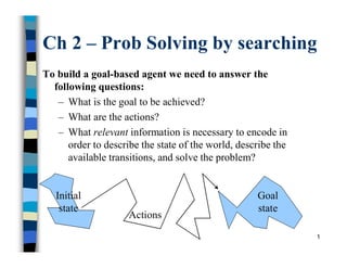
  • 1. 1 Ch 2 – Prob Solving by searching To build a goal-based agent we need to answer the following questions: – What is the goal to be achieved? – What are the actions? – What relevant information is necessary to encode in order to describe the state of the world, describe the available transitions, and solve the problem? Initial state Goal state Actions
  • 2. 2 What is the goal to be achieved?  Could describe a situation we want to achieve, a set of properties that we want to hold, etc.  Requires defining a “goal test” so that we know what it means to have achieved/satisfied our goal.
  • 3. 3 What are the actions?  Characterize the primitive actions or events that are available for making changes in the world in order to achieve a goal.  Deterministic world: no uncertainty in an action’s effects. Given an action (a.k.a. operator or move) and a description of the current world state, the action completely specifies – whether that action can be applied to the current world (i.e., is it applicable and legal), and – what the exact state of the world will be after the action is performed in the current world (i.e., no need for “history” information to compute the new world).
  • 4. 4 Representing actions Note also that actions in this framework can all be considered as discrete events that occur at an instant of time. –For example, if “Sita is in class” and then performs the action “go home,” then in the next situation she is “at home.” There is no representation of a point in time where she is neither in class nor at home (i.e., in the state of “going home”).
  • 5. 5 Representing actions The number of actions / operators depends on the representation used in describing a state. – In the 8-puzzle, we could specify 4 possible moves for each of the 8 tiles, resulting in a total of 4*8=32 operators. – On the other hand, we could specify four moves for the “blank” square and we would only need 4 operators. Representational shift can greatly simplify a problem!
  • 6. 6 Representing states  What information is necessary to encode about the world to sufficiently describe all relevant aspects in solving the goal? That is, what knowledge needs to be represented in a state description to adequately describe the current state or situation of the world?  The size of a problem is usually described in terms of the number of states that are possible. – Tic-Tac-Toe has about 39 states. – Checkers has about 1040 states. – Rubik’s Cube has about 1019 states. – Chess has about 10120 states in a typical game.
  • 7. 7 Defining a Problem as a State Space 1. Define a state space that contains all the possible configurations of the relevant objects. 2. Specify one (or more) state(s) as the initial state(s). 3. Specify one (or more) state(s) as the goal state(s). 4. Specify a set of rules that describe available actions (operators), considering:  What assumptions are present in the informal problem description?  How general should the rules be?  How much of work required to solve the problem should be precompiled and represented in the rules?
  • 8. 8 2.2.1 Production Systems  A set of rules (Knowledge Base) : – LHS  RHS (if-part  then-part) – Pattern  Action – Antecedent  Consequent  Knowledge containing information (temporary or permanent) required to solve the current task. (Working Memory)  A control strategy to specify the order of testing patterns and resolving possible conflicts (Inference Engine)  A rule applier.
  • 9. 9 Production System Major Components knowledge base – contains essential information about the problem domain – often represented as facts and rules inference engine – mechanism to derive new knowledge from the knowledge base and the information provided by the user – often based on the use of rules
  • 10. 10 Production (Rule-Based) System Knowledge Base Inference Engine Working Memory User Interface Agenda
  • 11. 11 Rule-Based System  knowledge is encoded as IF … THEN rules – these rules can also be written as production rules  the inference engine determines which rule antecedents are satisfied – the left-hand side must “match” a fact in the working memory  satisfied rules are placed on the agenda  rules on the agenda can be activated (“fired”) – an activated rule may generate new facts through its right-hand side – the activation of one rule may subsequently cause the activation of other rules
  • 12. 12 Example Rules IF … THEN Rules Rule: Red_Light IF the light is red THEN stop Rule: Green_Light IF the light is green THEN go antecedent (left-hand-side) consequent (right-hand-side) Production Rules the light is red ==> stop the light is green ==> go
  • 13. 13 Inference Engine Cycle  describes the execution of rules by the inference engine – match • update the agenda – add rules whose antecedents are satisfied to the agenda – remove non-satisfied rules from agendas – conflict resolution • select the rule with the highest priority from the agenda – execution • perform the actions on the consequent of the selected rule • remove the rule from the agenda  the cycle ends when – no more rules are on the agenda, or – an explicit stop command is encountered
  • 14. 14 The Water Jugs Problem  2 jugs – 5 gallon – 3 gallon  How can you get exactly 4 gallons into the 5 gallon jug?  Possible operators: – Empty jug – Fill jug from tap – Pour contents from one jug into another • Empty contents of one jug into the other • Transfer some of contents of one jug to fill-up the other 5 3
  • 15. The Water Jugs Problem 15
  • 16. Water Jugs Problem – Solution 1 16 Table 2.2 Solution Path 1 Rule Applied 5-g jug 3-g jug Step No Initial state 0 0 1 5 0 1 8 2 3 2 4 2 0 3 6 0 2 4 1 5 2 5 8 4 3 6 Goal state 4 -
  • 17. Water Jugs Problem – Solution 2 17 Table 2.2 Solution Path 2 Rule Applied 5-g jug 3-g jug Step No Initial state 0 0 3 0 3 1 5 3 0 2 3 3 3 3 7 5 1 4 2 0 1 5 5 1 0 6 3 1 3 7 5 4 0 8 Goal state 4 -
  • 18. Missionaries and Cannibals 18 RN Left side of rule  Right side of rule Rules for boat going from left bank to right bank of the river L1 ([n1M, m1C, 1B], [n2M, m2C, 0B])  ([(n1-2)M, m1C, 0B], [(n2+2)M, m2C, 1B]) L2 ([n1M, m1C, 1B], [n2M, m2C, 0B])  ([(n1-1)M,(m1-1)C,0B],[(n2+1)M,(m2+1)C, 1B]) L3 ([n1M, m1C, 1B], [n2M, m2C, 0B])  ([n1M, (m1-2)C, 0B], [n2M, (m2+2)C, 1B]) L4 ([n1M, m1C, 1B], [n2M, m2C, 0B])  ([(n1-1)M, m1C,0B],[(n2+1)M, m2C, 1B]) L5 ([n1M, m1C, 1B], [n2M, m2C, 0B])  ([n1M, (m1-1)C, 0B], [n2M, (m2+1)C, 1B]) Rules for boat coming from right bank to left bank of the river R1 ([n1M, m1C, 0B], [n2M, m2C, 1B])  ([(n1+2)M, m1C, 1B], [(n2-2)M, m2C, 0B]) R2 ([n1M, m1C, 0B], [n2M, m2C, 1B])  ([(n1+1)M,(m1+1)C,1B],[(n2-1)M,(m2-1)C, 0B]) R3 ([n1M, m1C, 0B], [n2M, m2C, 1B])  ([n1M, (m1+2)C, 1B], [n2M, (m2-2)C, 0B]) R4 ([n1M, m1C, 0B], [n2M, m2C, 1B])  ([(n1+1)M, m1C,1B],[(n2-1)M, m2C, 0B]) R5 ([n1M, m1C, 0B], [n2M, m2C, 1B])  ([n1M, (m1+1)C, 1B], [n2M, (m2-1)C, 0B])
  • 19. Missionaries and Cannibals - solution 19 Start  ([3M, 3C, 1B], [0M, 0C, 0B]] L2: ([2M, 2C, 0B], [1M, 1C, 1B]) R4: ([3M, 2C, 1B], [0M, 1C, 0B]) L3: ([3M, 0C, 0B], [0M, 3C, 1B]) R4: ([3M, 1C, 1B], [0M, 2C, 0B]) L1: ([1M, 1C, 0B], [2M, 2C, 1B]) R2: ([2M, 2C, 1B], [1M, 1C, 0B]) L1: ([0M, 2C, 0B], [3M, 1C, 1B]) R5: ([0M, 3C, 1B], [3M, 0C, 0B]) L3: ([0M, 1C, 0B], [3M, 2C, 1B]) R5: ([0M, 2C, 1B], [3M, 1C, 0B]) 1M,1C  1M  2C  1C  2M  1M,1C  2M  1C  2C  1C  L3: ([0M, 0C, 0B], [3M, 3C, 1B]) 2C  Goal state
  • 20. 20 2.2.2 State Space Search  State Space consists of 4 components 1. A set S of start (or initial) states 2. A set G of goal (or final) states 3. A set of nodes representing all possible states 4. A set of arcs connecting nodes representing possible actions in different states.
  • 21. Problem solving by search  Represent the problem as STATES and OPERATORS that transform one state into another state.  A solution to the problem is an OPERATOR SEQUENCE that transforms the INITIAL STATE into a GOAL STATE.  Finding the sequence requires SEARCHING the STATE SPACE by GENERATING the paths connecting the two. 21
  • 22. 22 Missionaries and Cannibals: Initial State and Actions  initial state: – all missionaries, all cannibals, and the boat are on the left bank  5 possible actions: – one missionary crossing – one cannibal crossing – two missionaries crossing – two cannibals crossing – one missionary and one cannibal crossing
  • 23. 23 Missionaries and Cannibals: State Space 1c 1m 1c 2c 1c 2c 1c 2m 1m 1c 1m 1c 1c 2c 1m 2m 1c 2c 1c 1m
  • 24. 24 Missionaries and Cannibals: Goal State and Path Cost  goal state: – all missionaries, all cannibals, and the boat are on the right bank.  path cost – step cost: 1 for each crossing – path cost: number of crossings = length of path  solution path: – 4 optimal solutions – cost: 11
  • 25. 25 Example: Measuring problem!  Problem: Using these three buckets, measure 7 liters of water. 3 l 5 l 9 l
  • 26. 26 Example: Measuring problem!  (1 possible) Solution: a b c 0 0 0 3 0 0 0 0 3 3 0 3 0 0 6 3 0 6 0 3 6 3 3 6 1 5 6 0 5 7 3 l 5 l 9 l a b c Initial state Goal state
  • 27. 27 Example: Measuring problem!  Another Solution: a b c 0 0 0 0 5 0 3 2 0 3 0 2 3 5 2 3 0 7 3 l 5 l 9 l a b c
  • 28. 28 Which solution do we prefer? • Solution 1: a b c 0 0 0 3 0 0 0 0 3 3 0 3 0 0 6 3 0 6 0 3 6 3 3 6 1 5 6 0 5 7 • Solution 2: a b c 0 0 0 0 5 0 3 2 0 3 0 2 3 5 2 3 0 7
  • 29. 29 8-queens • State: any arrangement of up to 8 queens on the board • Initial state: no queens on the board • Operation: add a queen to any empty square • Goal state: no queen is attacked (like the above board).
  • 30. 30 8-queens… Improved states • State: an arrangement of n (up to 8) queens, 1 each in the n leftmost columns • Operation: add a queen in leftmost empty column such that it is not attacked by the other queens. Improvement: Just 2057 possible states instead of P(64,8)  648
  • 31. 31 Control Strategies  Control strategy is one of the most important component of intelligent systems and specify the order in which rules are applied in a given current state.  A good control strategy should have the following properties: – Cause motion – Be systematic
  • 32. 32 Data/Goal-driven Strategies  Data-driven search = forward chaining. – Start from an initial state and work towards a goal state. – Examples seen so far  Goal-driven search = backward chaining. – Start from a goal state and work towards an initial state. – Prolog programming, theorem proving …
  • 33. 33 Seven problem characteristics 1. Decomposability of a problem  Towers of Hanoi 2. Can solution steps be ignored or undone?  Ignorable : theorem proving  Some of the lemmas proved can be ignored  Recoverable : 8 tile puzzle  solution steps can be undone (backtracking)  Irrecoverable : chess  solution steps can not be undone
  • 34. 34 3. Is the universe predictable? • 8-puzzel (yes) • Bridge/chess (no)  but we can use probabilities of each possible outcomes 4. Is a good solution absolute or relative? • More than one solution? • traveling salesman problem Seven problem characteristics
  • 35. 35 5. Is the solution a state or a path ? - Given a sequence of formulae, does a statement follow from them? - water jug problem  path / plan 6. What is the role of knowledge? knowledge for perfect program of chess (need knowledge to constrain the search) newspaper story understanding (need knowledge to recognize a solution) 7. Does the task require interaction with a person? solitary/ conversational Seven problem characteristics
  • 36. 36 Toy Problems vs. Real-World Problems Toy Problems – concise and exact description – used for illustration purposes (e.g. here) – used for performance comparisons – all the above examples Real-World Problems – no single, agreed- upon description – people care about the solutions (useful)
  • 37. 37 Real-World Problem: Touring in Romania Oradea Bucharest Fagaras Pitesti Neamt Iasi Vaslui Urziceni Hirsova Eforie Giurgiu Craiova Rimnicu Vilcea Sibiu Dobreta Mehadia Lugoj Timisoara Arad Zerind 120 140 151 75 70 111 118 75 71 85 90 211 101 97 138 146 80 99 87 92 142 98 86
  • 38. 38 Touring in Romania: Search Problem Definition  initial state: – In(Arad)  possible Actions: – DriveTo(Zerind), DriveTo(Sibiu), DriveTo(Timisoara), etc.  goal state: – In(Bucharest)  step cost: – distances between cities
  • 39. 39 Searching for solutions  An agent with several immediate options of unknown value can decide what to do by first examining different possible sequences of actions that lead to states of known value, and then choosing the best sequence.  search (through the state space) for • a goal state • a sequence of actions that leads to a goal state • a sequence of actions with minimal path cost that leads to a goal state
  • 40. 40 Search Trees  search tree: tree structure defined by initial state and successor function  Touring Romania (partial search tree): In(Arad) In(Zerind) In(Sibiu) In(Timisoara) In(Arad) In(Oradea) In(Fagaras) In(Rimnicu Vilcea) In(Sibiu) In(Bucharest)
  • 41. 41 Search Nodes  search nodes: the nodes in the search tree  data structure: – state: a state in the state space – parent node: the immediate predecessor in the search tree – action: the action that, performed in the parent node’s state, leads to this node’s state – path cost: the total cost of the path leading to this node – depth: the depth of this node in the search tree
  • 42. 42 Expanded Search Nodes in Touring Romania Example In(Arad) In(Zerind) In(Sibiu) In(Timisoara) In(Arad) In(Oradea) In(Fagaras) In(Rimnicu Vilcea) In(Sibiu) In(Bucharest)
  • 43. 43 Fringe Nodes in Touring Romania Example fringe nodes: nodes that have not been expanded In(Arad) In(Zerind) In(Sibiu) In(Timisoara) In(Arad) In(Oradea) In(Fagaras) In(Rimnicu Vilcea) In(Sibiu) In(Bucharest)
  • 44. 44 A General State-Space Search Algorithm open := {S}; closed :={}; repeat n := select(open); /* select one node from open for expansion */ if n is a goal then exit with success; /* delayed goal testing */ expand(n) /* generate all children of n put these newly generated nodes in open (check duplicates) put n in closed (to check duplicates) */ until open = {}; exit with failure
  • 45. 45 Key Features of the General Search Algorithm  systematic – guaranteed to not generate the same state infinitely often – guaranteed to come across every state eventually  incremental – attempts to reach a goal state step by step (rather than guessing it all at once)
  • 46. 46 In(Arad) In(Oradea) In(Rimnicu Vilcea) In(Zerind) In(Timisoara) In(Sibiu) In(Bucharest) In(Fagaras) In(Sibiu) General Search Algorithm: Touring Romania Example In(Arad) fringe selected
  • 47. 47 Evaluating Search Strategies • Completeness: Is it guaranteed that a solution will be found? • Optimality: Is the best solution found when several solutions exist? • Time complexity: How long does it take to find a solution? • Space complexity: How much memory is needed to perform a search? • Branching factor (b) 1 + b + b2 + b3 + ... + bd b nodes b nodes b nodes
  • 48. 48 Search Cost vs. Total Cost  search cost: – time (and memory) used to find a solution  total cost: – search cost + path cost of solution  optimal trade-off point: – further computation to find a shorter path becomes counterproductive
  • 49. 49 Uninformed vs. Informed Search  uninformed search (blind search) – no additional information about states beyond problem definition – only goal states and non-goal states can be distinguished – E.g., BFS, DFS, DFID, UCS,…  informed search (heuristic search) – additional information about how “promising” a state is available – Greedy HDFS, BeFs, A*, …
  • 50. 50 Breadth-First Search  strategy: – expand root node – expand successors of root node – expand successors of successors of root node – etc.  implementation: – use FIFO queue to store fringe nodes in general tree search algorithm
  • 51. 51 Breadth First Search Algorithm open := [Start]; // Initialize closed := [ ]; while open != [ ] // While states remain { remove the leftmost state from open, call it X; if X is a goal return success; // Success else { generate children of X; put X on closed; eliminate children of X on open or closed; // loops put remaining children at the END of open; } // QUEUE } return failure;
  • 52. 52 depth = 3 Breadth-First Search: Missionaries and Cannibals depth = 0 depth = 1 depth = 2
  • 53. 53 Breadth-First Search: Evaluation completeness yes optimality shallowest time complexity O(bd+1) space complexity O(bd+1)
  • 54. 54 Time complexity of BFS • If a goal node is found on depth d of the tree, all nodes up till that depth are created. G b d  Thus: O(bd+1)
  • 55. 55  In General: bd+1 Space complexity of BFS • Largest number of nodes in QUEUE is reached on the level d of the goal node. G b d
  • 56. 56 Exponential Complexity: Important Lessons  memory requirements are a bigger problem for breadth-first search than is the execution time  time requirements are still a major factor  exponential-complexity search problems cannot be solved by uninformed methods for any but the smallest instances
  • 57. 57 Depth-First Search  strategy: – always expand the deepest node in the current fringe first – when a sub-tree has been completely explored, delete it from memory and “back up”  implementation: – use LIFO queue (stack) to store fringe nodes in general tree search algorithm
  • 58. 58 Depth First Search Algorithm open := [Start]; // Initialize closed := [ ]; while open != [ ] // While states remain { remove the leftmost state from open, call it X; if X is a goal return success; // Success else { generate children of X; put X on closed; eliminate children of X on open or closed; // loops put remaining children at the START of open; } // STACK } return failure;
  • 59. 59 depth = 3 Depth-First Search: Missionaries and Cannibals depth = 0 depth = 1 depth = 2
  • 60. 60 Depth-First Search: Evaluation completeness no optimality no time complexity O(bd+1) space complexity O(bd)
  • 61. 61 Time complexity of DFS • In the worst case: • the goal node may be on the right-most branch, G d b  Time complexity O(bd+1)
  • 62. 62 Space complexity of DFS • Largest number of nodes in QUEUE is reached in bottom left-most node. ...  Order: O(b*d)
  • 63. 63 Evaluation of Depth-first & Breadth-first • Completeness: Is it guaranteed that a solution will be found? • Yes for BFS • No for DFS • Optimality: Is the best solution found when several solutions exist? • No for both BFS and DFS if edges are of different length • Yes for BFS and No for DFS if edges are of same length • Time complexity: How long does it take to find a solution? • Worst case: both exponential • Average case: DFS is better than BFS • Space complexity: How much memory is needed to perform a search? • Exponential for BFS • Linear for DFS
  • 64. 64 Depth-first vs Breadth-first  Use depth-first when – Space is restricted – High branching factor – There are no solutions with short paths – No infinite paths  Use breadth-first when – Possible infinite paths – Some solutions have short paths – Low branching factor
  • 65. 65 Depth-First Iterative Deepening (DFID)  BF and DF both have exponential time complexity O(bd) BF is complete but has exponential space complexity DF has linear space complexity but is incomplete  Space is often a harder resource constraint than time  Can we have an algorithm that – is complete and – has linear space complexity ?  DFID by Korf in 1987 First do DFS to depth 0 (i.e., treat start node as having no successors), then, if no solution found, do DFS to depth 1, etc. until solution found do DFS with depth bound c c = c+1
  • 66. 66 depth = 3 Iterative Deepening Search: Missionaries and Cannibals depth = 0 depth = 1 depth = 2
  • 67. 67 Depth-First Iterative Deepening (DFID)  Complete (iteratively generate all nodes up to depth d)  Optimal if all operators have the same cost. Otherwise, not optimal but does guarantee finding solution of fewest edges (like BF).  Linear space complexity: O(bd), (like DF)  Time complexity is exponential O(bd), but a little worse than BFS or DFS because nodes near the top of the search tree are generated multiple times.  Worst case time complexity is exponential for all blind search algorithms !
  • 68. 68 Iterative Deepening Search: Evaluation completeness yes optimality shallowest time complexity O(bd) space complexity O(bd)
  • 69. 69 Uniform/Lowest-Cost (UCS/LCFS)  BFS, DFS, DFID do not take path cost into account.  Let g(n) = cost of the path from the start node to an open node n  Algorithm outline: – Always select from the OPEN the node with the least g(.) value for expansion, and put all newly generated nodes into OPEN – Nodes in OPEN are sorted by their g(.) values (in ascending order) – Terminate if a node selected for expansion is a goal  Called “Dijkstra's Algorithm” in the algorithms literature and similar to “Branch and Bound Algorithm” in operations research literature
  • 70. 70 A Uniform-cost Search Algorithm open := {S}; closed :={}; repeat n := select(open); /* select the 1st node from open for expansion */ if n is a goal then exit with success; /* delayed goal testing */ expand(n) /* generate all children of n put these newly generated nodes in open (check duplicates) sort open (by path cost g(n)) put n in closed (check duplicates) */ until open = {}; exit with failure
  • 71. 71 UCS example A D B E C F G S 3 4 4 4 5 5 4 3 2 AFTER open closed ITERATION 0 [S(0)] [ ] 1 [A(3), D(4)] [S(0)] 2 [D(4), B(7)] [S(0), A(3)] 3 [E(6), B(7)] [S(0), A(3), D(4)] 4 [B(7), F(10)] [S(0), A(3), D(4), E(6)] 5 [F(10), C(11)] 6 [C(11), G(13)] 7 [G(13)]
  • 72. 72 Uniform-Cost -- analysis Complete (if cost of each edge is not infinitesimal) – The total # of nodes n with g(n) ≤ g(goal) in the state space is finite – Goal node will eventually be generated (put in OPEN) and selected for expansion (and passes the goal test) Optimal – When the first goal node is selected for expansion (and passes the goal test), its path cost is less than or equal to g(n) of every OPEN node n (and solutions entailed by n) Exponential time and space complexity, O(bd) where d is the depth of the solution path of the least cost solution
  • 73. 73 Bidirectional Search  idea: run two simultaneous searches: – one forward from the initial state, – one backward from the goal state, until the two fringes meet. The solution path must cross the meeting point. Start Goal
  • 74. 74 Bidirectional Search: Caveats  What search strategy for forward/backward search? – breadth-first search  How to check whether a node is in the other fringe? – hash table  must know goal state for backward search  must be able to compute predecessors and successors for a given state
  • 75. 75 Bidirectional Search: Evaluation completeness yes optimality shallowest time complexity O(bd/2) space complexity O(bd/2)
  • 76. 76 Comparing Uninformed Search Strategies Breadth -First Uniform- Cost Depth- First Depth- Limite d Iterative Deepening Bidirectiona l Breadth-F. complete? Yes Yes No No Yes Yes optimal? Yes Yes No No Yes Yes time complexity O(bd+1) O(b1+⌊C*/ε⌋) O(bd+1) O(bl) O(bd) O(bd/2) space complexity O(bd+1) O(b1+⌊C*/ε⌋) O(bd) O(bl) O(bd) O(bd/2)
  • 77. 77 When to use what Depth-First Search: – Space is limited – High branching factor – No infinite branches Breadth-First Search: – Some solutions are known to be shallow Iterative-Deepening Search: – Space is limited and the shortest solution path is required Uniform-Cost Search: – Actions have varying costs – Least cost solution is the required The only uninformed search that worries about costs.
  • 78. 78 Repeated states  Repeated states can be a source of great inefficiency: identical subtrees will be explored many times! – Failure to detect repeated states can turn a linear problem into an exponential one ! How much effort to invest in detecting repetitions?
  • 79. 79 Strategies for repeated states  Do not expand the state that was just generated – constant time, prevents cycles of length one, ie., A,B,A,B….  Do not expand states that appear in the path – time linear in the depth of node, prevents some cycles of the type A,B,C,D,A  Do not expand states that were expanded before – can be expensive! Use hash table to avoid looking at all nodes every time.
  • 80. 80 Summary: uninformed search  Problem formulation and representation is key! – State formulation with care (8-queens) – Action formulation with care (8-puzzle)  Implementation as expanding directed graph of states and transitions  Appropriate for problems where no solution is known and many combinations must be tried  Problem space is of exponential size in the number of world states -- NP-hard problems  Fails due to lack of space and/or time.
  • 81. Homework 1. Explain the seven characteristics of AI problems. 2. Define state space search. 3. Compare the search strategies BFS, DFS, DFID, UCS, based time complexity, space complexity, optimality and completeness. 4. A farmer is stranded on an island with 3 of his belongings: cabbage, goat and tiger. He has a small boat capable of carrying him and one of his belongings. He cannot leave cabbage and goat unattended (the cabbage will be eaten by the goat) and cannot leave tiger and goat unattended (the tiger will eat the goat). Design a state-space representation for this search problem and draw the state- space showing the first 3 levels. 81
  • 82. Homework 5. In the rabbit leap problem, three east-bound rabbits stand in a line blocked by three west-bound rabbits as shown below. They are crossing a stream with stones placed in a line. A rabbit can only move forward or jump over one rabbit to get to an unoccupied stone. Design a state-space representation for this search problem and draw the state-space showing the first 3 levels. Find a solution path in the state space. 82