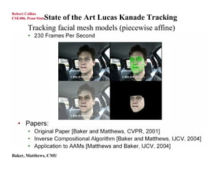
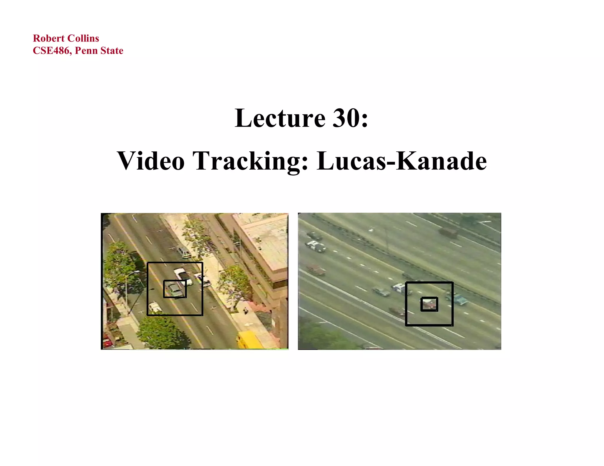
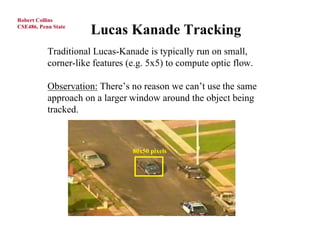
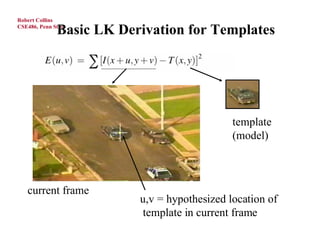
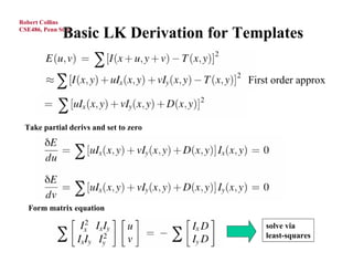
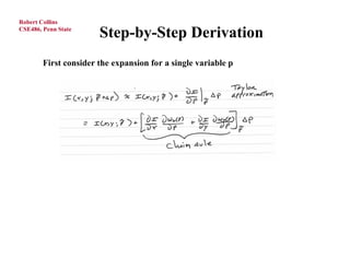
The document discusses the Lucas-Kanade template tracking method. It begins with a review of Lucas-Kanade optical flow, then describes how the same approach can be used to track larger image patches or templates by imposing the constraint that neighboring pixels have similar motion. It presents the derivation step-by-step, showing how a Taylor series approximation allows formulation as a least squares problem. An example Jacobian for affine motion models is provided. The algorithm iterates between warping the template, computing error, estimating motion parameters, and updating. State-of-the-art examples include tracking facial mesh models.


![Robert Collins
CSE486, Penn State
One Problem with this...
Assumption of constant flow (pure translation) for
all pixels in a larger window is unreasonable for
long periods of time.
However, we can easily generalize Lucas-Kanade
approach to other 2D parametric motion models
(like affine or projective) by introducing a “warp”
function W.
generalize
x
[ I (W ([ x, y ]; P)) T ([ x, y ])]2
within image patch
y
](https://image.slidesharecdn.com/lecture30-110524024940-phpapp02/85/Lecture30-9-320.jpg)
![Robert Collins
CSE486, Penn State
Step-by-Step Derivation
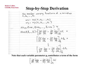
The key to the derivation is Taylor series approximation:
W
[ I (W ([ x, y ]; P P)) ~ [ I (W ([ x, y ]; P)) I
~ P
P
We will derive this step-by-step. First, we need two background formula:](https://image.slidesharecdn.com/lecture30-110524024940-phpapp02/85/Lecture30-10-320.jpg)
![Robert Collins
CSE486, Penn State
Step-by-Step Derivation
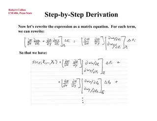
Further collecting the dw/dpi terms into a matrix, we can write:
which are the terms in the matrix equation:
~ W
[ I (W ([ x, y ]; P P)) ~ [ I (W ([ x, y ]; P)) I P
P](https://image.slidesharecdn.com/lecture30-110524024940-phpapp02/85/Lecture30-14-320.jpg)
![Robert Collins
Example: Jacobian of Affine Warp
CSE486, Penn State
Let W([x, y]; P) [Wx , Wy ]
general equation of Jacobian Wx Wx Wx Wx
W P P P P
1 2 3 n
P Wy Wy Wy Wy
P
1 P2 P3 P
n
affine warp function (6 parameters)
x xP yP3 P5
1
x W xP2 y yP4 P6
1 p1
W ([ x, y ]; P )
p3 p5
y
p6 P P
p2 1 p4 1
x 0 y 0 1 0
0 x 0 y 0 1 ](https://image.slidesharecdn.com/lecture30-110524024940-phpapp02/85/Lecture30-15-320.jpg)
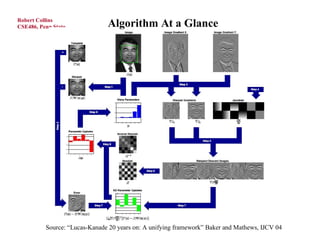
![Source: “Lucas-Kanade 20 years on: A unifying framework” Baker and Mathews, IJCV 04
Robert Collins
CSE486, Penn State
Iterate Warp I to obtain I(W([x y];P))
Compute the error image T(x) – I(W([x y]; P))
Warp the gradient I with W([x y]; P)
W
Evaluate at ([x y]; P) (Jacobian)
P
W
Compute steepest descent images I
P
W T W
Compute Hessian matrix (I P
) (I
P
)
W T
Compute ( I P
) (T ( x, y ) I (W ([ x, y ]; P )))
Compute P
Update P P + P
Until P magnitude is negligible
Dr. Ng Teck Khim](https://image.slidesharecdn.com/lecture30-110524024940-phpapp02/85/Lecture30-16-320.jpg)