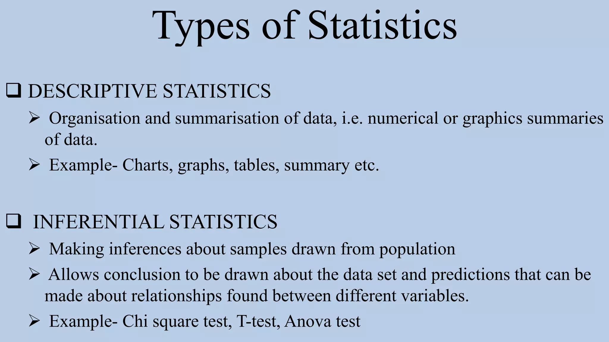
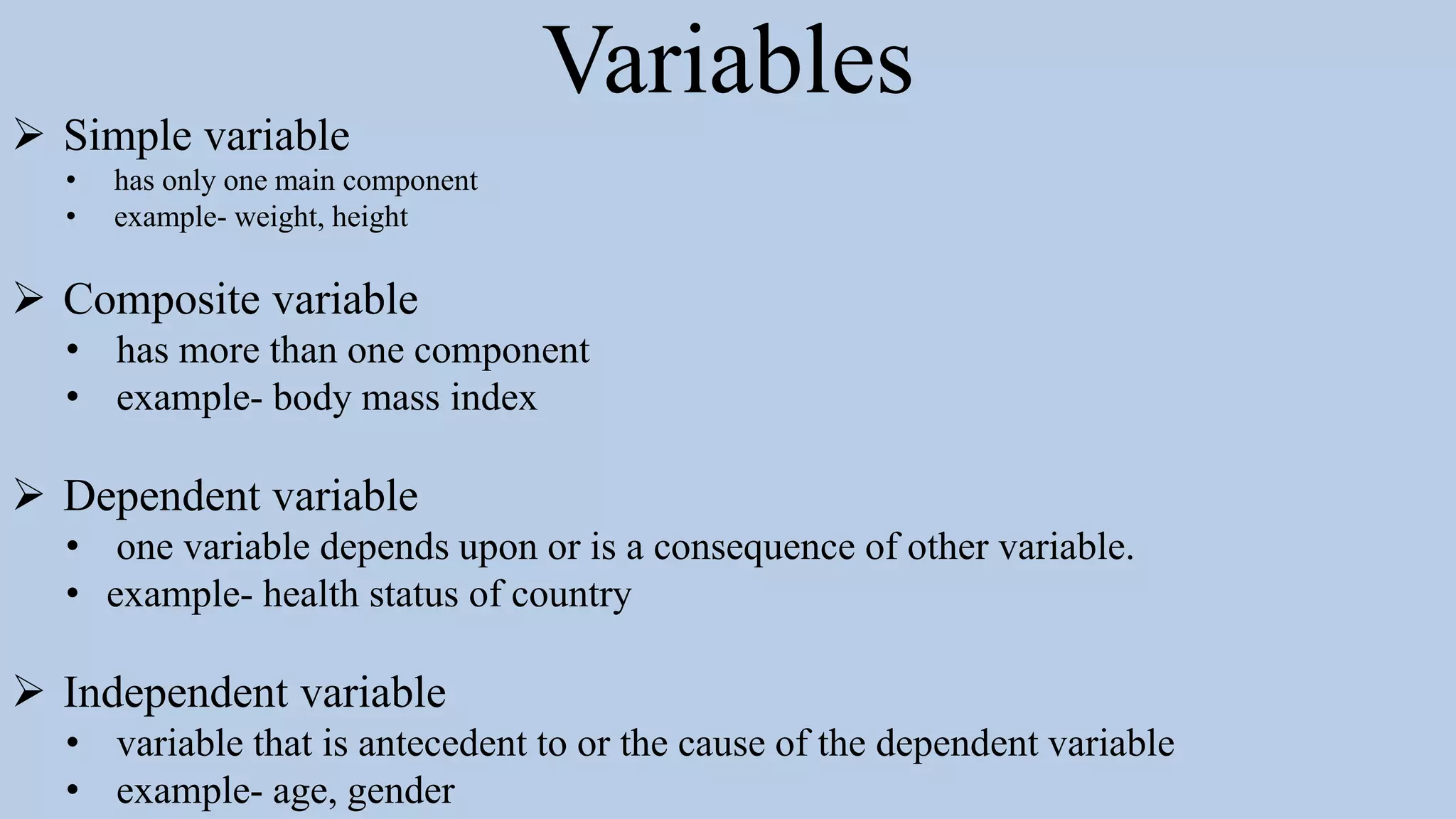
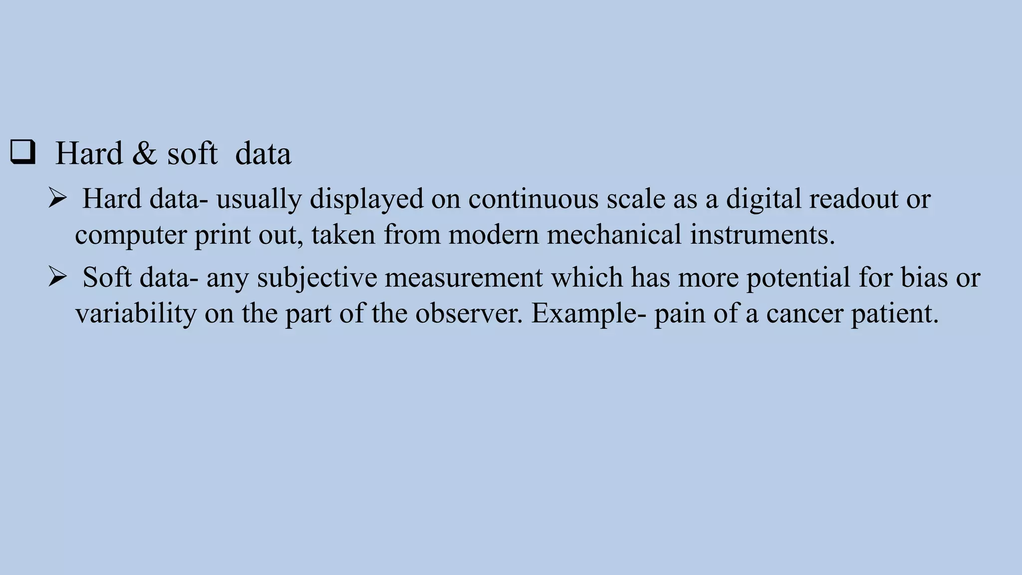
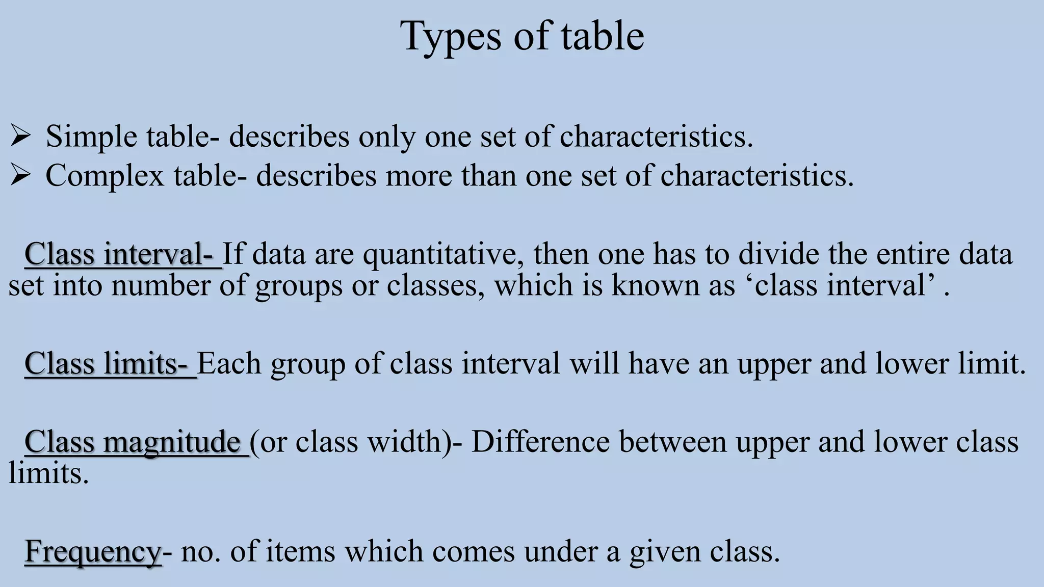
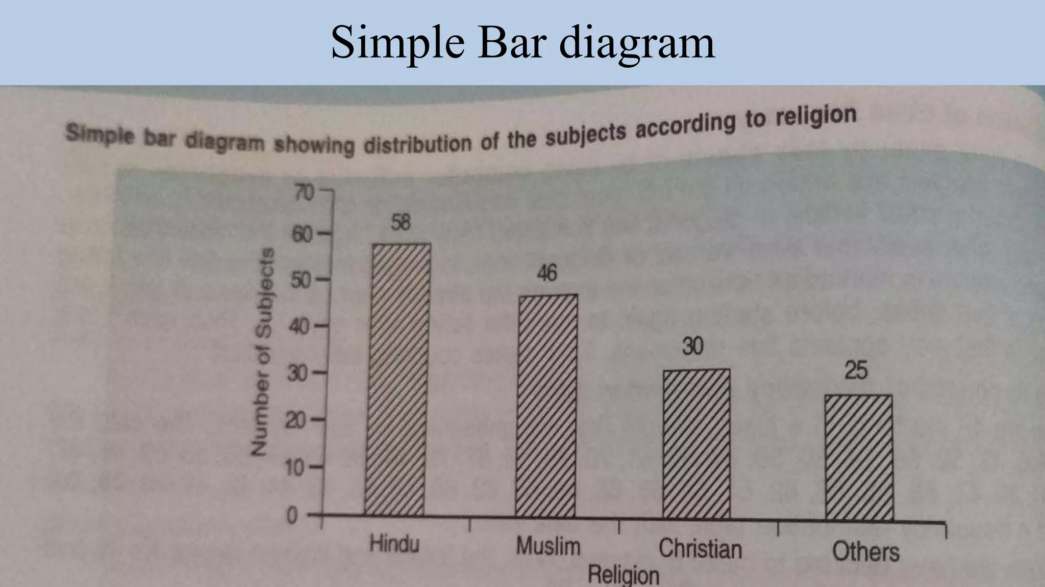
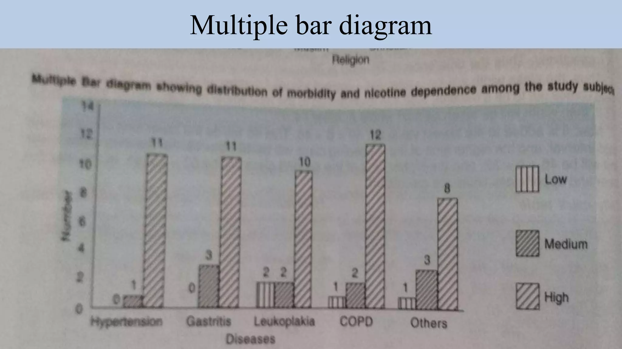
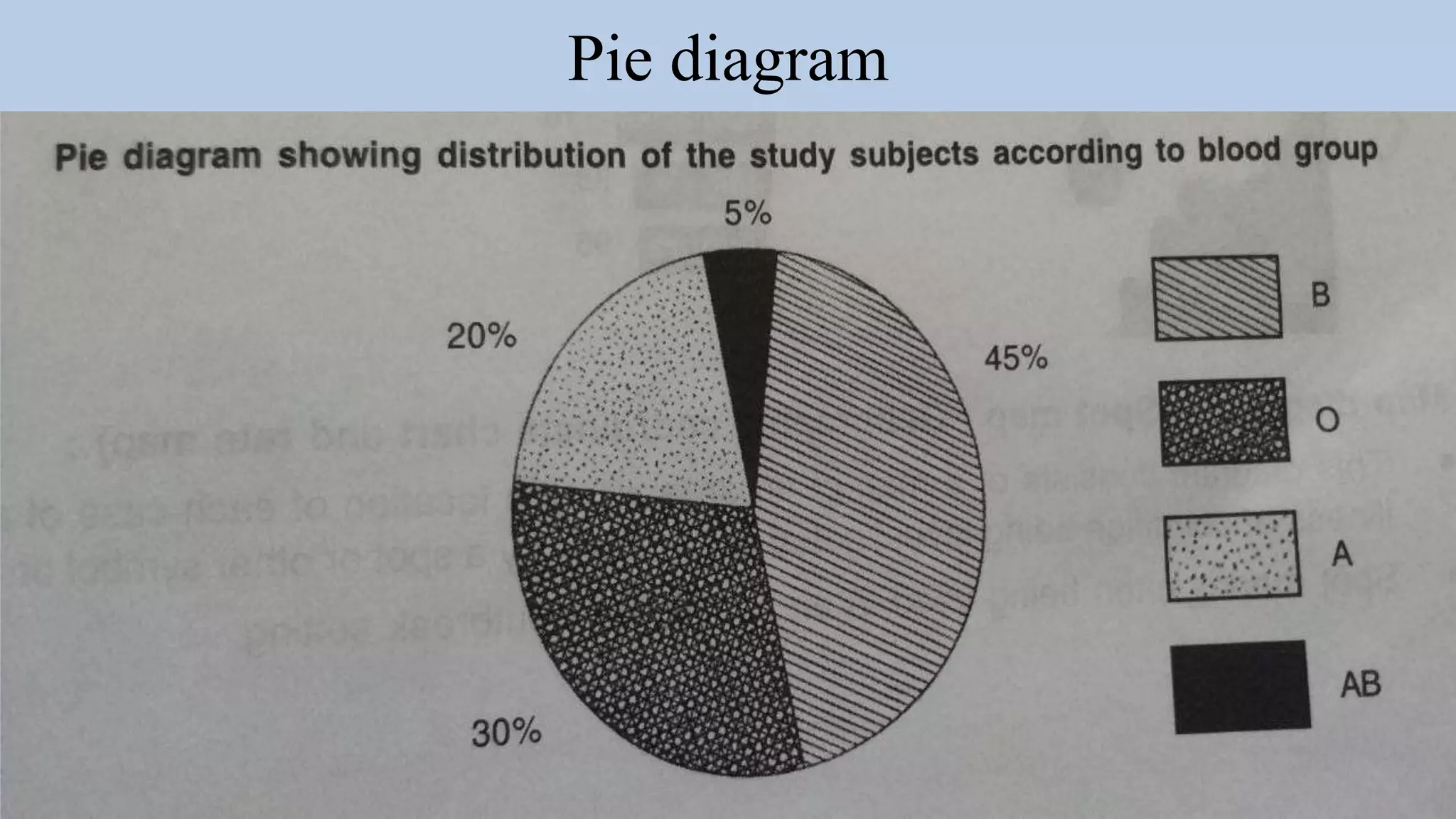
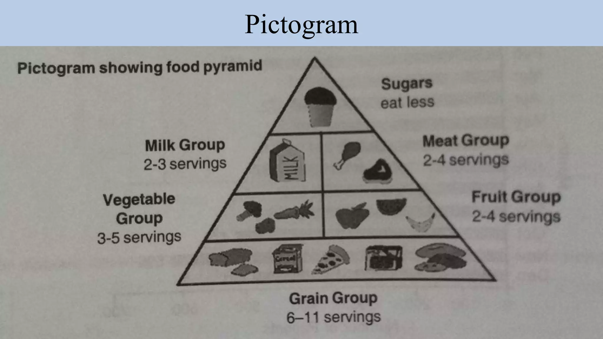
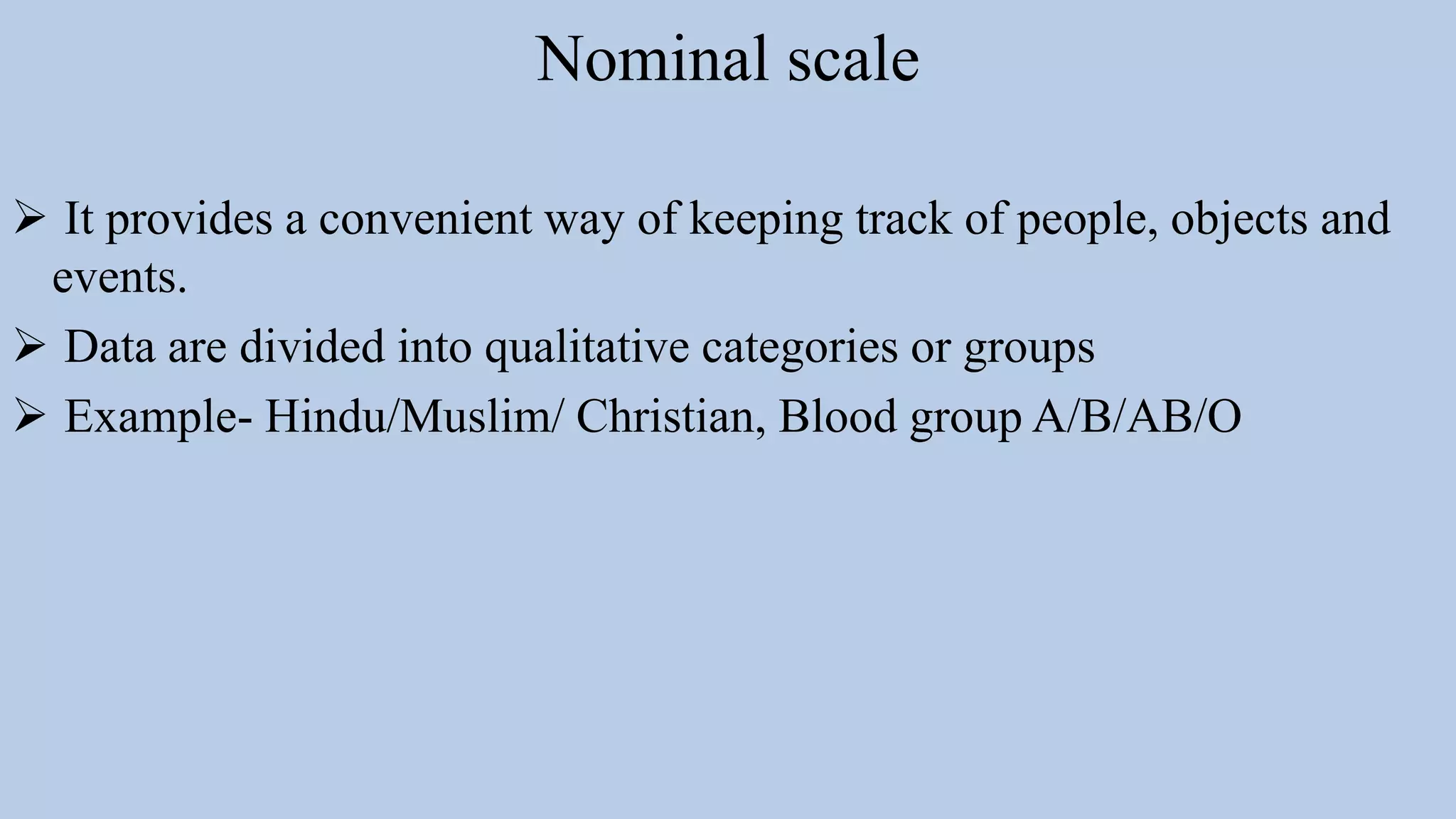
IMPORTANCE OF
STATISTICS
Dr. Bipul Borthakur (Professor)
Dept of Orthopaedics,
SMCH
Introduction
 Statistics is a field of study concerned with collection, organisation,
summarisation and analysis of data and the drawing of inferences about a body
when only a part of data are observed.
 In other words, it is the scientific methodology of decision making from
collected data or information.
Types of Statistics
 DESCRIPTIVE STATISTICS
 Organisation and summarisation of data, i.e. numerical or graphics summaries
of data.
 Example- Charts, graphs, tables, summary etc.
 INFERENTIAL STATISTICS
 Making inferences about samples drawn from population
 Allows conclusion to be drawn about the data set and predictions that can be
made about relationships found between different variables.
 Example- Chi square test, T-test, Anova test
Variables
 Simple variable
• has only one main component
• example- weight, height
 Composite variable
• has more than one component
• example- body mass index
 Dependent variable
• one variable depends upon or is a consequence of other variable.
• example- health status of country
 Independent variable
• variable that is antecedent to or the cause of the dependent variable
• example- age, gender
Variables
 Latent variable
• the variable which cannot be measured directly but assumed to be related to a no. of
observations
• example- bright student, efficient worker.
 Random variable
• when value cannot be predicted in advance
• example- tossing a coin
 Attribute-
• qualitative character of an event is referred to as attribute.
• example- sex, religion,
Data
 Data are facts expressed in numerical terms
 Information
• When data set undergoes through statistical processing, it becomes
information.
 Intelligence
• It is for the decision or policy makers based on transformation of the
information.
Classification of data
Data can be classified in various ways.
 Continuous & Discrete data
 Continuous is data for which an unlimited no. of possible values exist. Example is height and
weight
 Discrete data is data for which limited no. of variable exist. Example- no. of players in a cricket
team.
 Qualitative & quantitative data
 Qualitative data- which can’t be measured, but can be expressed in frequency, example- sex,
religion.
 Quantitative data- characteristic and the frequency of a variable can be measured, example- height,
weight.
 Primary & secondary data
 Primary data- collected by researcher themselves, example- census data, field survey
 Secondary data- which has been collected by someone else and are used by another researcher.
 Hard & soft data
 Hard data- usually displayed on continuous scale as a digital readout or
computer print out, taken from modern mechanical instruments.
 Soft data- any subjective measurement which has more potential for bias or
variability on the part of the observer. Example- pain of a cancer patient.
Presentation of data
Data can be presented in two ways
 Diagrammatic
 Tabular
Tabular presentation
 Different parts of table
• table number
• title (heading)
• caption (individual column/heads/boxhead)
• stubhead
• stub
• body (data field)
• footnote
• sources
Types of table
 Simple table- describes only one set of characteristics.
 Complex table- describes more than one set of characteristics.
Class interval- If data are quantitative, then one has to divide the entire data
set into number of groups or classes, which is known as ‘class interval’ .
Class limits- Each group of class interval will have an upper and lower limit.
Class magnitude (or class width)- Difference between upper and lower class
limits.
Frequency- no. of items which comes under a given class.
Graphic representation
Diagrams for qualitative/categorial/discrete data
 Bar diagram:
• Different categories are indicated on one axis and frequency of data in each category is
indicated on the other axis and categories are compared by length of bars.
• Three different types of bar diagram- simple, multiple and component bar diagram.
 Pie diagram
• It is used to represent division of whole into segments by using wedge-shaped portions of a
circle for comparison.
• Degrees of angle denote the frequency and area of sector.
 Pictogram
• Small pictures or symbols are used to represent the diagram that conveys some statistical
information.
 Map diagram
• This consists of a map of an area with location of each case of an event.
 Venn diagram
• This shows the degree of overlap and exclusively for two or more
characteristics or factors within a sample, or population, or for a characteristic
among two or more samples.
Simple Bar diagram
Multiple bar diagram
Component bar diagram
Pie diagram
Pictogram
Map diagram
Venn diagram
Quantitative data
 Histogram
 Frequency polygon
 Frequency curve
 Line chart
 Cumulative frequency
 Scatter diagram
 Box plot
 Stem and Leaf plot/Stem plot
 Spider Chart
Histogram
Frequency polygon
Frequency curve
Line chart
Cumulative frequency
Scatter diagram
Box plot
Stem and Leaf plot/Stem plot
Spider chart
Scales of measurements
Four different measurement scales
 Nominal
 Ordinal
 Interval
 Ratio
Nominal scale
 It provides a convenient way of keeping track of people, objects and
events.
 Data are divided into qualitative categories or groups
 Example- Hindu/Muslim/ Christian, Blood group A/B/AB/O
Ordinal scale
 This scale places events in a meaningful order i.e. observations are
ordered or ranked on the basis of specific characteristics.
 Example- Acute respiratory infection may be classified as no
pneumonia, pneumonia, severe pneumonia
Interval scale
 Similar to ordinal scale, here data are placed in meaningful order and
in addition they have definite interval between them.
 Example- In Celsius scale, difference between 100 degree and degree.
Ratio scale
 This scale has some properties as an interval scale; nut because it has
an absolute zero, meaningful ratios do exist.
 Example- weight in grams or pounds, time in seconds or days.
THANK YOU
“sukhaduḥkhe same kṛtvā lābhālābhau jayājayau
tato yuddhāya yujyasva naivaṃ pāpamavāpsyasi”
“Holding pleasure and pain, gain and loss, victory and defeat as
alike, gird yourself up for the battle.
Thus, you shall not incur any sin.”

Biostatistics pt 1

  • 1.
    IMPORTANCE OF STATISTICS Dr. BipulBorthakur (Professor) Dept of Orthopaedics, SMCH
  • 2.
    Introduction  Statistics isa field of study concerned with collection, organisation, summarisation and analysis of data and the drawing of inferences about a body when only a part of data are observed.  In other words, it is the scientific methodology of decision making from collected data or information.
  • 3.
    Types of Statistics DESCRIPTIVE STATISTICS  Organisation and summarisation of data, i.e. numerical or graphics summaries of data.  Example- Charts, graphs, tables, summary etc.  INFERENTIAL STATISTICS  Making inferences about samples drawn from population  Allows conclusion to be drawn about the data set and predictions that can be made about relationships found between different variables.  Example- Chi square test, T-test, Anova test
  • 4.
    Variables  Simple variable •has only one main component • example- weight, height  Composite variable • has more than one component • example- body mass index  Dependent variable • one variable depends upon or is a consequence of other variable. • example- health status of country  Independent variable • variable that is antecedent to or the cause of the dependent variable • example- age, gender
  • 5.
    Variables  Latent variable •the variable which cannot be measured directly but assumed to be related to a no. of observations • example- bright student, efficient worker.  Random variable • when value cannot be predicted in advance • example- tossing a coin  Attribute- • qualitative character of an event is referred to as attribute. • example- sex, religion,
  • 6.
    Data  Data arefacts expressed in numerical terms  Information • When data set undergoes through statistical processing, it becomes information.  Intelligence • It is for the decision or policy makers based on transformation of the information.
  • 7.
    Classification of data Datacan be classified in various ways.  Continuous & Discrete data  Continuous is data for which an unlimited no. of possible values exist. Example is height and weight  Discrete data is data for which limited no. of variable exist. Example- no. of players in a cricket team.  Qualitative & quantitative data  Qualitative data- which can’t be measured, but can be expressed in frequency, example- sex, religion.  Quantitative data- characteristic and the frequency of a variable can be measured, example- height, weight.  Primary & secondary data  Primary data- collected by researcher themselves, example- census data, field survey  Secondary data- which has been collected by someone else and are used by another researcher.
  • 8.
     Hard &soft data  Hard data- usually displayed on continuous scale as a digital readout or computer print out, taken from modern mechanical instruments.  Soft data- any subjective measurement which has more potential for bias or variability on the part of the observer. Example- pain of a cancer patient.
  • 9.
    Presentation of data Datacan be presented in two ways  Diagrammatic  Tabular
  • 10.
    Tabular presentation  Differentparts of table • table number • title (heading) • caption (individual column/heads/boxhead) • stubhead • stub • body (data field) • footnote • sources
  • 11.
    Types of table Simple table- describes only one set of characteristics.  Complex table- describes more than one set of characteristics. Class interval- If data are quantitative, then one has to divide the entire data set into number of groups or classes, which is known as ‘class interval’ . Class limits- Each group of class interval will have an upper and lower limit. Class magnitude (or class width)- Difference between upper and lower class limits. Frequency- no. of items which comes under a given class.
  • 12.
    Graphic representation Diagrams forqualitative/categorial/discrete data  Bar diagram: • Different categories are indicated on one axis and frequency of data in each category is indicated on the other axis and categories are compared by length of bars. • Three different types of bar diagram- simple, multiple and component bar diagram.  Pie diagram • It is used to represent division of whole into segments by using wedge-shaped portions of a circle for comparison. • Degrees of angle denote the frequency and area of sector.  Pictogram • Small pictures or symbols are used to represent the diagram that conveys some statistical information.
  • 13.
     Map diagram •This consists of a map of an area with location of each case of an event.  Venn diagram • This shows the degree of overlap and exclusively for two or more characteristics or factors within a sample, or population, or for a characteristic among two or more samples.
  • 14.
  • 15.
  • 16.
  • 17.
  • 18.
  • 19.
  • 20.
  • 21.
    Quantitative data  Histogram Frequency polygon  Frequency curve  Line chart  Cumulative frequency  Scatter diagram  Box plot  Stem and Leaf plot/Stem plot  Spider Chart
  • 22.
  • 23.
  • 24.
  • 25.
  • 26.
  • 27.
  • 28.
  • 29.
    Stem and Leafplot/Stem plot
  • 30.
  • 31.
    Scales of measurements Fourdifferent measurement scales  Nominal  Ordinal  Interval  Ratio
  • 32.
    Nominal scale  Itprovides a convenient way of keeping track of people, objects and events.  Data are divided into qualitative categories or groups  Example- Hindu/Muslim/ Christian, Blood group A/B/AB/O
  • 33.
    Ordinal scale  Thisscale places events in a meaningful order i.e. observations are ordered or ranked on the basis of specific characteristics.  Example- Acute respiratory infection may be classified as no pneumonia, pneumonia, severe pneumonia
  • 34.
    Interval scale  Similarto ordinal scale, here data are placed in meaningful order and in addition they have definite interval between them.  Example- In Celsius scale, difference between 100 degree and degree.
  • 35.
    Ratio scale  Thisscale has some properties as an interval scale; nut because it has an absolute zero, meaningful ratios do exist.  Example- weight in grams or pounds, time in seconds or days.
  • 36.
    THANK YOU “sukhaduḥkhe samekṛtvā lābhālābhau jayājayau tato yuddhāya yujyasva naivaṃ pāpamavāpsyasi” “Holding pleasure and pain, gain and loss, victory and defeat as alike, gird yourself up for the battle. Thus, you shall not incur any sin.”