
Downloaded 17 times


![36
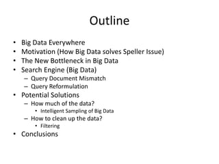
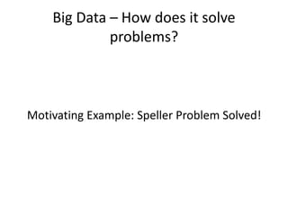
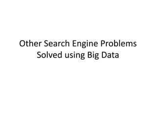
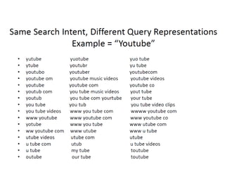
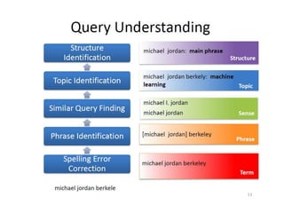
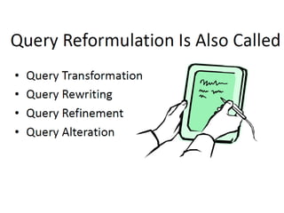
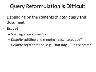
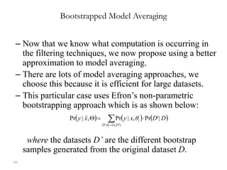
The Curse of Large Datasets
There are two main challenges of dealing with large datasets.
• Running Time: Reducing the amount of time it takes for the mining
algorithm to train.
• Predictive Accuracy: Poor quality of instances in training data lead
to lower predictive accuracies. Large datasets are usually
heterogeneous, and subjected to more noisy instances [Liu, Motoda
DMKD 2002].
The goal of our work is to address these questions and provide some
solutions.](https://image.slidesharecdn.com/bigdatacolloquiumtalk-150416152757-conversion-gate01/85/Big-Data-Challenges-and-Solutions-36-320.jpg)
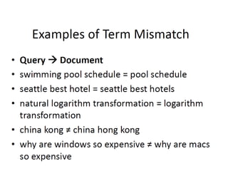
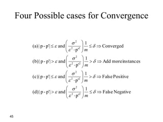
![38
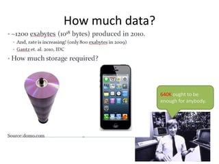
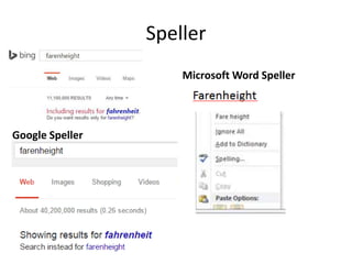
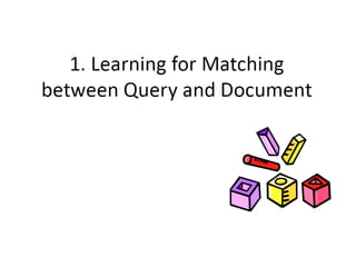
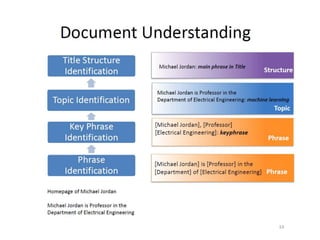
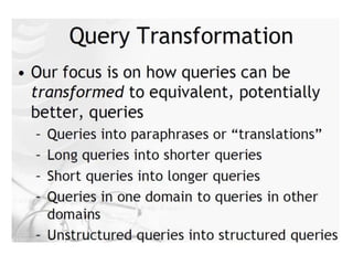
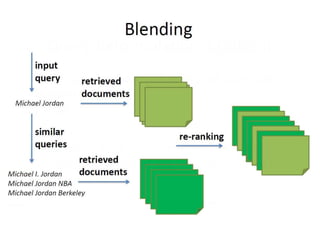
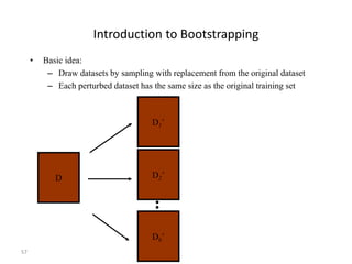
Learning Curve Phenomenon
• Is it necessary to apply learner
to all of the available data?
• A learning curve depicts the
relationship between sample
size and accuracy [Provost,
Jensen & Oates 99].
• Problem: Determining nmin efficiently
Given a data mining algorithm M, a dataset D of N instances, we would like the
smallest sample Di of size nmin such that:
Pr(acc(D) – acc(Di) > ε) ≤ δ
ε is the maximum acceptable decrease in accuracy (approximation) and
δ is the probability of failure](https://image.slidesharecdn.com/bigdatacolloquiumtalk-150416152757-conversion-gate01/85/Big-Data-Challenges-and-Solutions-38-320.jpg)
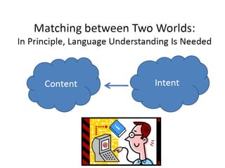
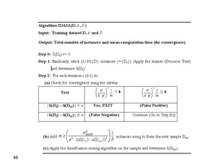
![39
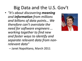
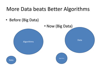
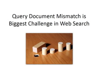
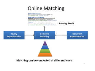
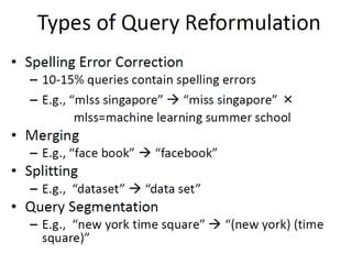
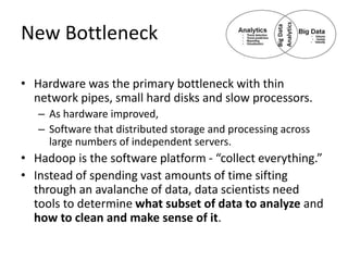
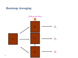
Prior Work: Static Sampling
• Arithmetic Sampling [John & Langley
KDD 1996] uses a schedule
Sa = <n0, n0 + nδ, n0 + 2nδ,..n0+k.nδ>
Example: An example arithmetic
schedule is <100 , 200, 300, . . . .>
Drawback: If nmin is a large multiple of
nδ, then the approach will require many
runs of the underlying algorithm.
The total number of instances used may
be greater than N.](https://image.slidesharecdn.com/bigdatacolloquiumtalk-150416152757-conversion-gate01/85/Big-Data-Challenges-and-Solutions-39-320.jpg)
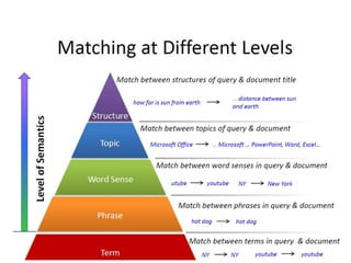
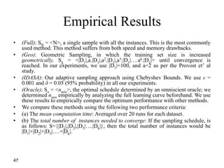
![40
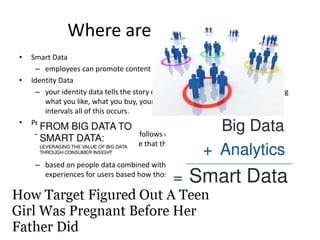
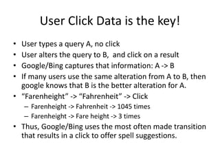
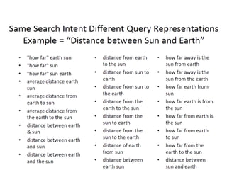
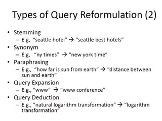
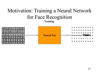
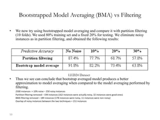
Prior Work in Progressive Sampling
• Geometric Sampling [Provost, Jenson &
Oates KDD 1999] uses a schedule
Sg= <n0, a.n0,a2.n0, ………,ak.n0>
An example geometric schedule is:
<100,200,400,800, . . .>
Drawbacks:
(a) In practice, Geometric Sampling
suffers from overshooting nmin.
(b) Not dependent on the dataset at
hand. A good sampling algorithm
is expected to have low bias and
low sampling variance
For example in the KDD CUP dataset,
when nmin=56,600,
the geometric schedule is as follows:
{100, 200, 400, 800, 1600, 3200, 6400,
12800, 25600, 51200, 102400}.
Notice here that the last sample has
overshot nmin by 45,800 instances](https://image.slidesharecdn.com/bigdatacolloquiumtalk-150416152757-conversion-gate01/85/Big-Data-Challenges-and-Solutions-40-320.jpg)
![42
Definition: Chebyshev Inequality
• Definition 1: Chebyshev Inequality [Bertrand and Chebyshev-1845]: In any
probability distribution, the probability of the estimated quantity p’ being more than
epsilon far away from the true value p after m independently drawn points is
bounded by:
m
1
p'
]|p'-p|Pr[ 22
2
m
1
p'
]|p'-p|Pr[ 22
2
What are we trying to solve?
Pr(acc(D) – acc(Dnmin) > ε) ≤ δ
Challenge: how do we compute the accuracy of the entire dataset acc(D)?](https://image.slidesharecdn.com/bigdatacolloquiumtalk-150416152757-conversion-gate01/85/Big-Data-Challenges-and-Solutions-42-320.jpg)
![Myopic Strategy: One Step at a time
43
û(Di)
û(Di+1)
||
1
)(
||
1
)
i
û(D
iD
i
i
i
xf
D
[Average over the sample Di]
The instance function f(xi) used here is a
Bernoulli trial, 0-1 classification accuracy](https://image.slidesharecdn.com/bigdatacolloquiumtalk-150416152757-conversion-gate01/85/Big-Data-Challenges-and-Solutions-43-320.jpg)
![44
m
1
p'
]|p'-p|Pr[ 22
2
True value
u(Da)-u(Db);
where |Da|>|Db|>nmin
Estimated value
u(Da)-u(Db);
where |Da|>|Db|≥1
Plateau Region:
p=0
Myopic Strategy:
u(Di) - u(Di-1)
m
BOOT 1
))u(D-)u(D(
)u(D-)u(D-0Pr 2
1-ii
2
2
1-ii
1
))u(D-)u(D( 2
1-ii
2
2
BOOT
m
m
BOOT 1
))u(D-)u(D( 2
1-ii
2
2
Approximation parameter
Confidence parameter
Bootstrapped Variance p’
(to improve the quality of the training data)](https://image.slidesharecdn.com/bigdatacolloquiumtalk-150416152757-conversion-gate01/85/Big-Data-Challenges-and-Solutions-44-320.jpg)
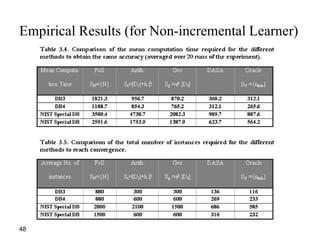


![54
Bayesian Analysis of Filtering
Techniques
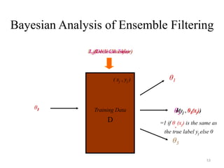
• Bayesian Analysis of Ensemble Filtering:
– Ensemble Filtering [Brodley & Friedl 1999- JAIR]: An ensemble classifier detects
mislabeled instances by constructing a set of classifiers (m base level detectors).
– A majority vote filter tags an instance as mislabeled if more than half of the m
classifiers classify it incorrectly
– If < ½ then the instance is noisy and is removed
– Example: Say δ(yj ,θ1(xj)) =1 (non-noisy)
δ(yj ,θ2(xj)) =0 (noisy)
δ(yj ,θ3(xj)) =0 (noisy)
Pr(y|x,Θ*) = 1/3 =0.33 < ½ , The instance xj is treated as noisy and is removed.
*
,
||
1
),|Pr( *
*
xtxty
),|Pr( *
xty](https://image.slidesharecdn.com/bigdatacolloquiumtalk-150416152757-conversion-gate01/85/Big-Data-Challenges-and-Solutions-54-320.jpg)
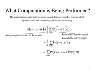
![60
Why remove noise?
• 1) Removing noisy instances increases
the predictive accuracy. This has been
shown by Quinlan [Qui86] and Brodley
and Friedl ([BF96][BF99])
• 2) Removing noisy instances creates a
simpler model. We show this empirically
in the Table.
• 3) Removing noisy instances reduces the
variance of the predictive accuracy: This
makes a more stable learner whose
accuracy estimate is more likely to be the
true value.](https://image.slidesharecdn.com/bigdatacolloquiumtalk-150416152757-conversion-gate01/85/Big-Data-Challenges-and-Solutions-60-320.jpg)
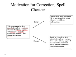

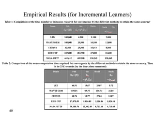
The document discusses big data challenges and potential solutions. It begins by outlining how big data is generated from various sources and used in applications like search engines. The main challenges are determining which subset of big data to analyze and how to clean noisy data. Two potential solutions discussed are: 1) Intelligent sampling to determine a representative subset of data to analyze instead of the entire dataset, in order to improve running time. Adaptive sampling techniques like IDASA are proposed. 2) Filtering techniques like ensemble filtering use multiple models to identify and remove mislabeled instances from training data, in order to improve predictive accuracy by cleaning the data. Bayesian analysis can interpret filtering as a form of model averaging.


![[243] turning data into value](https://cdn.slidesharecdn.com/ss_thumbnails/234turningdataintovalue-150915052705-lva1-app6891-thumbnail.jpg?width=640&height=640&fit=bounds)


![Getting Started with Apache Spark: Big Data Made Simple [Free Meetup]](https://cdn.slidesharecdn.com/ss_thumbnails/apachesparkgettingstarted-260203175547-8361bcc3-thumbnail.jpg?width=640&height=640&fit=bounds)


