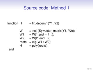
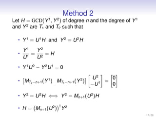
Blind FIR system identification
using a greatest common divisor
approach
Mayank and Ivan Markovsky
Dept. ELEC, Vrije Universiteit Brussel
1 / 20
Outline
• The blind system identification problem
• Greatest common divisor methods
2 / 20
Blind system identification
• Finite impulse response (FIR) system
y = u ∗ h
y(t) = (u ∗ h)(t) =
n
τ=0
h(τ) u(t − τ), t = 0, . . . , Ty
• Blind system identification: given y, find u and h
• Ill-posed problem: there are infinitely many solutions
3 / 20
Two experiments
20 40 60 80
−1
0
1
10 20 30 40
−1
0
1
20 40 60 80
−0.2
0
0.2
10 20 30 40
−1
0
1
4 / 20
Question: (y1
, y2
) → h
20 40 60 80
−1
0
1
20 40 60 80
−0.2
0
0.2
5 / 20
Answer: GCD(Y1
, Y2
) ↔ h
20 40 60 80
−1
0
1
20 40 60 80
−0.2
0
0.2
6 / 20
Z-transform
U(z) = Z(u) =
Tu
t=0
u(t)z−t
Convolution property. Let U, H and Y be the Z-tranform
of signals u, h and y, respectively
y = u ∗ h ⇐⇒ Y = U H
7 / 20
Greatest common divisor (GCD)
Let
Y1
=
T1
i=0
y1
i zi
and Y2
=
T2
i=0
y2
i zi
The GCD of Y1
and Y2
is a highest possible degree
polynomial, that is a factor of both Y1
and Y2
Example 1. Let
Y1
= z3
− 1 = (z − 1)(z2
+ z + 1),
Y2
= z3
+ 2z2
+ 2z + 1 = (z + 1)(z2
+ z + 1)
GCD(Y1
, Y2
) = z2
+ z + 1
8 / 20
Main result
Theorem. Let
yi
= ui
∗ h, for i = 1, 2,
where inputs u1
and u2
have finite support. Let U1
, U2
and Y1
, Y2
are the Z-transform of the input signals u1
, u2
and output signal y1
, y2
respectively. If input polynomials
U1
and U2
have no common roots, then
h = α Z−1
GCD(Y1
, Y2
) , α ∈ R
9 / 20
Link to linear algebra: Multiplication matrix
U H = Y















u0
u1 u0
... u1
...
un−1
...
... u0
un un−1
... u1
un
...
...
... un−1
un















Mn+1(U)





h0
h1
...
hn





=





y0
y1
...
yTy





10 / 20
Vandermonde matrix
• For the vector z = (z1, . . . , zn)
VT (z) =





(z1)0
(z2)0
· · · (zn)0
(z1)1
(z2)1
· · · (zn)1
...
...
...
...
(z1)T
(z2)T
· · · (zn)T





11 / 20
Shifting property of Vandermonde matrix





(z1)0
· · · (zn)0
(z1)1
· · · (zn)1
...
...
...
(z1)T−1
· · · (zn)T−1





VT (z)



z1
...
zn



diag(z)
=





(z1)1
· · · (zn)1
(z1)2
· · · (zn)2
...
...
...
(z1)T
· · · (zn)T





VT (z)
VT (z) diag(z) = VT (z)
12 / 20
Sylvester matrix
S (Y1
, Y2
) = MT2
(Y1
) MT1
(Y2
)
=















y1
0 y2
0
y1
1 y1
0 y2
1 y2
0
... y1
1
...
... y2
1
...
y1
n−1
...
... y1
0 y2
n−1
...
... y2
0
y1
n y1
n−1
... y1
1 y2
n y2
n−1
... y2
1
y1
n
...
... y2
n
...
...
... y1
n−1
... y2
n−1
y1
n y2
n















13 / 20
Lemma 1.
• deg GCD(Y1
, Y2
) = T1 + T2 − rank S(Y1
, Y2
)
dim ker(S(Y1,Y2))
Lemma 2. If ker S(Y1
, Y2
) = span(w1, . . . , wn),
there exist z = (z1, . . . , zn) such that,
• w1 · · · wd
W
G = VT (z), for some nonsingular G
• GCD(Y1
, Y2
) =
n
i=1
(z − zi)
14 / 20
Method 1: [w1 · · · wn] → (z1, . . . , zn)
• Let ker S(Y1)
, Y2
) = span(w1, . . . , wn)
• Define W = [w1 · · · wn], WG = VT (z)
• WG diag(z) = WG ← Shift-property
• WG diag(z) = WG
• G diag(z) G−1
= W†
W
• eig(W†
W) = (z1, . . . , zn) ← roots of the GCD
• H =
n
i=1
(z − zi)
15 / 20
Source code: Method 1
function H = fir_deconv1(Y1, Y2)
W = null (Sylvester_matrix(Y1, Y2));
W1 = W(1:end − 1, :);
W2 = W(2: end, :);
roots = eig(W1  W2);
H = poly(roots );
end
16 / 20
Method 2
Let H = GCD(Y1
, Y2
) of degree n and the degree of Y1
and Y2
are T1 and T2 such that
• Y1
= U1
H and Y2
= U2
H
•
Y1
U1
=
Y2
U2
= H
• Y1
U2
− Y2
U1
= 0
• MT2−n+1(Y1
) MT1−n+1(Y2
)
U2
−U1 =
0
0
• Y2
= U2
H ⇐⇒ Y2
= Mn+1(U2
)H
• H = Mn+1(U2
)
†
Y2
17 / 20
Source code: Method 2
function H = fir_deconv2(Y1, Y2)
M_Y1 = Multiplication_matrix (Y1, T2 − d + 1);
M_Y2 = Multiplication_matrix (Y2, T1 − d + 1);
M = [M_Y1 M_Y2];
z = null (M);
n = T2 + T1 − rank(Sylvester_matrix(Y1, Y2));
U2 = z(1:T2 − n + 1);
M_U2 = Multiplication_matrix (U2, n + 1);
H = M_U2  Y2;
end
18 / 20
Elapsed time: O(T3
y )
0 200 400 600 800 1000
−1
0
1
2
3
4
5
length of the signals Ty
Time(sec)
Method 1
Theoretical time
0 200 400 600 800 1000
−1
0
1
2
3
4
length of the signals Ty
Time(sec)
Method 2
Theoretical time
5
19 / 20
Future work
• Extend the GCD approach for the Blind FIR system
Identification to
• Noisy data
• Multivariate systems
20 / 20

BeneluxPPT

  • 1.
    Blind FIR systemidentification using a greatest common divisor approach Mayank and Ivan Markovsky Dept. ELEC, Vrije Universiteit Brussel 1 / 20
  • 2.
    Outline • The blindsystem identification problem • Greatest common divisor methods 2 / 20
  • 3.
    Blind system identification •Finite impulse response (FIR) system y = u ∗ h y(t) = (u ∗ h)(t) = n τ=0 h(τ) u(t − τ), t = 0, . . . , Ty • Blind system identification: given y, find u and h • Ill-posed problem: there are infinitely many solutions 3 / 20
  • 4.
    Two experiments 20 4060 80 −1 0 1 10 20 30 40 −1 0 1 20 40 60 80 −0.2 0 0.2 10 20 30 40 −1 0 1 4 / 20
  • 5.
    Question: (y1 , y2 )→ h 20 40 60 80 −1 0 1 20 40 60 80 −0.2 0 0.2 5 / 20
  • 6.
    Answer: GCD(Y1 , Y2 )↔ h 20 40 60 80 −1 0 1 20 40 60 80 −0.2 0 0.2 6 / 20
  • 7.
    Z-transform U(z) = Z(u)= Tu t=0 u(t)z−t Convolution property. Let U, H and Y be the Z-tranform of signals u, h and y, respectively y = u ∗ h ⇐⇒ Y = U H 7 / 20
  • 8.
    Greatest common divisor(GCD) Let Y1 = T1 i=0 y1 i zi and Y2 = T2 i=0 y2 i zi The GCD of Y1 and Y2 is a highest possible degree polynomial, that is a factor of both Y1 and Y2 Example 1. Let Y1 = z3 − 1 = (z − 1)(z2 + z + 1), Y2 = z3 + 2z2 + 2z + 1 = (z + 1)(z2 + z + 1) GCD(Y1 , Y2 ) = z2 + z + 1 8 / 20
  • 9.
    Main result Theorem. Let yi =ui ∗ h, for i = 1, 2, where inputs u1 and u2 have finite support. Let U1 , U2 and Y1 , Y2 are the Z-transform of the input signals u1 , u2 and output signal y1 , y2 respectively. If input polynomials U1 and U2 have no common roots, then h = α Z−1 GCD(Y1 , Y2 ) , α ∈ R 9 / 20
  • 10.
    Link to linearalgebra: Multiplication matrix U H = Y                u0 u1 u0 ... u1 ... un−1 ... ... u0 un un−1 ... u1 un ... ... ... un−1 un                Mn+1(U)      h0 h1 ... hn      =      y0 y1 ... yTy      10 / 20
  • 11.
    Vandermonde matrix • Forthe vector z = (z1, . . . , zn) VT (z) =      (z1)0 (z2)0 · · · (zn)0 (z1)1 (z2)1 · · · (zn)1 ... ... ... ... (z1)T (z2)T · · · (zn)T      11 / 20
  • 12.
    Shifting property ofVandermonde matrix      (z1)0 · · · (zn)0 (z1)1 · · · (zn)1 ... ... ... (z1)T−1 · · · (zn)T−1      VT (z)    z1 ... zn    diag(z) =      (z1)1 · · · (zn)1 (z1)2 · · · (zn)2 ... ... ... (z1)T · · · (zn)T      VT (z) VT (z) diag(z) = VT (z) 12 / 20
  • 13.
    Sylvester matrix S (Y1 ,Y2 ) = MT2 (Y1 ) MT1 (Y2 ) =                y1 0 y2 0 y1 1 y1 0 y2 1 y2 0 ... y1 1 ... ... y2 1 ... y1 n−1 ... ... y1 0 y2 n−1 ... ... y2 0 y1 n y1 n−1 ... y1 1 y2 n y2 n−1 ... y2 1 y1 n ... ... y2 n ... ... ... y1 n−1 ... y2 n−1 y1 n y2 n                13 / 20
  • 14.
    Lemma 1. • degGCD(Y1 , Y2 ) = T1 + T2 − rank S(Y1 , Y2 ) dim ker(S(Y1,Y2)) Lemma 2. If ker S(Y1 , Y2 ) = span(w1, . . . , wn), there exist z = (z1, . . . , zn) such that, • w1 · · · wd W G = VT (z), for some nonsingular G • GCD(Y1 , Y2 ) = n i=1 (z − zi) 14 / 20
  • 15.
    Method 1: [w1· · · wn] → (z1, . . . , zn) • Let ker S(Y1) , Y2 ) = span(w1, . . . , wn) • Define W = [w1 · · · wn], WG = VT (z) • WG diag(z) = WG ← Shift-property • WG diag(z) = WG • G diag(z) G−1 = W† W • eig(W† W) = (z1, . . . , zn) ← roots of the GCD • H = n i=1 (z − zi) 15 / 20
  • 16.
    Source code: Method1 function H = fir_deconv1(Y1, Y2) W = null (Sylvester_matrix(Y1, Y2)); W1 = W(1:end − 1, :); W2 = W(2: end, :); roots = eig(W1 W2); H = poly(roots ); end 16 / 20
  • 17.
    Method 2 Let H= GCD(Y1 , Y2 ) of degree n and the degree of Y1 and Y2 are T1 and T2 such that • Y1 = U1 H and Y2 = U2 H • Y1 U1 = Y2 U2 = H • Y1 U2 − Y2 U1 = 0 • MT2−n+1(Y1 ) MT1−n+1(Y2 ) U2 −U1 = 0 0 • Y2 = U2 H ⇐⇒ Y2 = Mn+1(U2 )H • H = Mn+1(U2 ) † Y2 17 / 20
  • 18.
    Source code: Method2 function H = fir_deconv2(Y1, Y2) M_Y1 = Multiplication_matrix (Y1, T2 − d + 1); M_Y2 = Multiplication_matrix (Y2, T1 − d + 1); M = [M_Y1 M_Y2]; z = null (M); n = T2 + T1 − rank(Sylvester_matrix(Y1, Y2)); U2 = z(1:T2 − n + 1); M_U2 = Multiplication_matrix (U2, n + 1); H = M_U2 Y2; end 18 / 20
  • 19.
    Elapsed time: O(T3 y) 0 200 400 600 800 1000 −1 0 1 2 3 4 5 length of the signals Ty Time(sec) Method 1 Theoretical time 0 200 400 600 800 1000 −1 0 1 2 3 4 length of the signals Ty Time(sec) Method 2 Theoretical time 5 19 / 20
  • 20.
    Future work • Extendthe GCD approach for the Blind FIR system Identification to • Noisy data • Multivariate systems 20 / 20