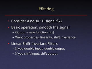
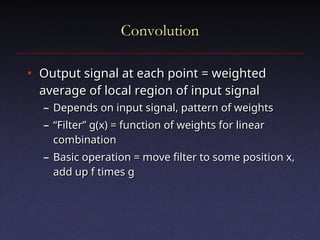
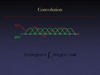
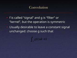
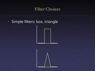
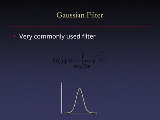
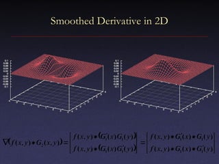
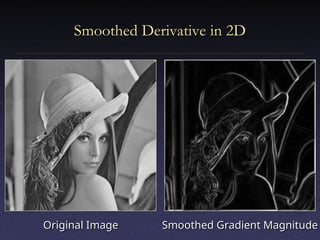
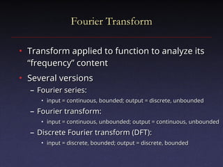
The document discusses digital signal processing, emphasizing concepts like filtering, convolution, and sampling to manage noisy signals. It explains the properties of linear shift-invariant filters and introduces Gaussian filters, highlighting their applications and advantages in smoothing signals. Additionally, the document covers Fourier transforms, detailing their role in analyzing frequency content and simplifying convolutions in signal processing.

1. Signal Processing
Signal Processing
COS 323
COS 323

2. Digital “Signals”
Digital “Signals”
• 1D: functions of space or time (e.g., sound)
1D: functions of space or time (e.g., sound)
• 2D: often functions of 2 spatial dimensions
2D: often functions of 2 spatial dimensions
(e.g. images)
(e.g. images)
• 3D: functions of 3 spatial dimensions
3D: functions of 3 spatial dimensions
(CAT, MRI scans) or 2 space, 1 time (video)
(CAT, MRI scans) or 2 space, 1 time (video)

3. Digital Signal Processing
Digital Signal Processing
1.
1. Understand analogues of
Understand analogues of filters
filters
2.
2. Understand nature of
Understand nature of sampling
sampling

4. Filtering
Filtering
• Consider a noisy 1D signal f(x)
Consider a noisy 1D signal f(x)
• Basic operation: smooth the signal
Basic operation: smooth the signal
– Output = new function h(x)
Output = new function h(x)
– Want properties: linearity, shift invariance
Want properties: linearity, shift invariance
• Linear Shift-Invariant Filters
Linear Shift-Invariant Filters
– If you double input, double output
If you double input, double output
– If you shift input, shift output
If you shift input, shift output

5. Convolution
Convolution
• Output signal at each point = weighted
Output signal at each point = weighted
average of local region of input signal
average of local region of input signal
– Depends on input signal, pattern of weights
Depends on input signal, pattern of weights
– “
“Filter” g(x) = function of weights for linear
Filter” g(x) = function of weights for linear
combination
combination
– Basic operation = move filter to some position x,
Basic operation = move filter to some position x,
add up f times g
add up f times g

6. Convolution
Convolution






 dt
t
x
g
t
f
x
g
x
f )
(
)
(
)
(
)
(
f(x)
f(x)
g(x)
g(x)

7. Convolution
Convolution
• f is called “signal” and g is “filter” or
f is called “signal” and g is “filter” or
“kernel”, but the operation is symmetric
“kernel”, but the operation is symmetric
• Usually desirable to leave a constant signal
Usually desirable to leave a constant signal
unchanged: choose g such that
unchanged: choose g such that
1
)
( 




dt
t
g

8. Filter Choices
Filter Choices
• Simple filters: box, triangle
Simple filters: box, triangle

9. Gaussian Filter
Gaussian Filter
• Very commonly used filter
Very commonly used filter
2
2
2
2
1
)
( 


x
e
x
G



10. Gaussian Filters
Gaussian Filters
• Gaussians are used because:
Gaussians are used because:
– Smooth (infinitely differentiable)
Smooth (infinitely differentiable)
– Decay to zero rapidly
Decay to zero rapidly
– Simple analytic formula
Simple analytic formula
– Separable: multidimensional Gaussian =
Separable: multidimensional Gaussian =
product of Gaussians in each dimension
product of Gaussians in each dimension
– Convolution of 2 Gaussians = Gaussian
Convolution of 2 Gaussians = Gaussian
– Limit of applying multiple filters is Gaussian
Limit of applying multiple filters is Gaussian
(Central limit theorem)
(Central limit theorem)

11. 2D Gaussian Filter
2D Gaussian Filter

12. Sampled Signals
Sampled Signals
• Can’t store continuous signal: instead store
Can’t store continuous signal: instead store
“samples”
“samples”
– Usually evenly sampled:
Usually evenly sampled:
f
f0
0=f(x
=f(x0
0), f
), f1
1=f(x
=f(x0
0+
+
x), f
x), f2
2=f(x
=f(x0
0+2
+2
x), f
x), f3
3=f(x
=f(x0
0+3
+3
x), …
x), …
• Instantaneous measurements of continuous
Instantaneous measurements of continuous
signal
signal
– This can lead to problems
This can lead to problems



13. Aliasing
Aliasing
• Reconstructed signal might be very
Reconstructed signal might be very
different from original: “aliasing”
different from original: “aliasing”
• Solution: smooth the signal
Solution: smooth the signal before
before sampling
sampling

 


14. Discrete Convolution
Discrete Convolution
• Integral becomes sum over samples
Integral becomes sum over samples
• Normalization condition is
Normalization condition is
 


i
i
x
i g
f
g
f
1


i
i
g

15. Computing Discrete Convolutions
Computing Discrete Convolutions
• What happens near edges of signal?
What happens near edges of signal?
– Ignore (Output is smaller than input)
Ignore (Output is smaller than input)
– Pad with zeros (edges get dark)
Pad with zeros (edges get dark)
– Replicate edge samples
Replicate edge samples
– Wrap around
Wrap around
– Reflect
Reflect
– Change filter
Change filter
 


i
i
x
i g
f
g
f

16. Computing Discrete Convolutions
Computing Discrete Convolutions
• If f has
If f has n
n samples and g has
samples and g has m
m nonzero
nonzero
samples,
samples,
straightforward computation takes time
straightforward computation takes time
O(
O(nm
nm)
)
• OK for small filter kernels, bad for large ones
OK for small filter kernels, bad for large ones
 


i
i
x
i g
f
g
f

17. Example: Smoothing
Example: Smoothing
Original image
Original image Smoothed with
Smoothed with
2D Gaussian kernel
2D Gaussian kernel

18. Example: Smoothed Derivative
Example: Smoothed Derivative
• Derivative of noisy signal = more noisy
Derivative of noisy signal = more noisy
• Solution: smooth with a Gaussian
Solution: smooth with a Gaussian
before
before taking derivative
taking derivative
• Differentiation and convolution both linear
Differentiation and convolution both linear
operators: they “commute”
operators: they “commute”
 
dx
dg
f
g
dx
df
g
f
dx
d






19. Example: Smoothed Derivative
Example: Smoothed Derivative
• Result: good way of finding derivative =
Result: good way of finding derivative =
convolution with derivative of Gaussian
convolution with derivative of Gaussian

20. Smoothed Derivative in 2D
Smoothed Derivative in 2D
• What is “derivative” in 2D? Gradient:
What is “derivative” in 2D? Gradient:
• Gaussian is separable!
Gaussian is separable!
• Combine smoothing, differentiation:
Combine smoothing, differentiation:














y
f
x
f
y
x
f ,
)
,
(
 
 
  

























)
(
)
(
)
,
(
)
(
)
(
)
,
(
)
(
)
(
)
,
(
)
(
)
(
)
,
(
)
,
(
)
,
(
1
1
1
1
1
1
1
1
2
y
G
x
G
y
x
f
y
G
x
G
y
x
f
y
G
x
G
y
x
f
y
G
x
G
y
x
f
y
x
G
y
x
f
)
(
)
(
)
,
( 1
1
2 y
G
x
G
y
x
G 

21. Smoothed Derivative in 2D
Smoothed Derivative in 2D
 
 
  

























)
(
)
(
)
,
(
)
(
)
(
)
,
(
)
(
)
(
)
,
(
)
(
)
(
)
,
(
)
,
(
)
,
(
1
1
1
1
1
1
1
1
2
y
G
x
G
y
x
f
y
G
x
G
y
x
f
y
G
x
G
y
x
f
y
G
x
G
y
x
f
y
x
G
y
x
f

22. Smoothed Derivative in 2D
Smoothed Derivative in 2D
Original Image
Original Image Smoothed Gradient Magnitude
Smoothed Gradient Magnitude

23. Canny Edge Detector
Canny Edge Detector
• Smooth
Smooth
• Find derivative
Find derivative
• Find maxima
Find maxima
• Threshold
Threshold

24. Canny Edge Detector
Canny Edge Detector
Original Image
Original Image Edges
Edges

25. Fourier Transform
Fourier Transform
• Transform applied to function to analyze its
Transform applied to function to analyze its
“frequency” content
“frequency” content
• Several versions
Several versions
– Fourier series:
Fourier series:
• input = continuous, bounded; output = discrete, unbounded
input = continuous, bounded; output = discrete, unbounded
– Fourier transform:
Fourier transform:
• input = continuous, unbounded; output = continuous, unbounded
input = continuous, unbounded; output = continuous, unbounded
– Discrete Fourier transform (DFT):
Discrete Fourier transform (DFT):
• input = discrete, bounded; output = discrete, bounded
input = discrete, bounded; output = discrete, bounded

26. Fourier Series
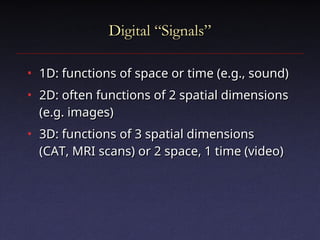
Fourier Series
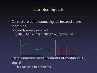
• Periodic function f(x) defined over [–
Periodic function f(x) defined over [–
 ..
.. 
 ]
]
where
where






1
0
2
1
)
sin(
)
cos(
)
(
n
n
n nx
b
nx
a
a
x
f












dx
nx
x
f
b
dx
nx
x
f
a
n
n
)
sin(
)
(
)
cos(
)
(
1
1

27. Fourier Series
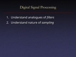
Fourier Series
• This works because sines, cosines are
This works because sines, cosines are
orthonormal over [–
orthonormal over [–
 ..
.. 
 ]:
]:
• Kronecker delta:
Kronecker delta:


 










otherwise
0
if
1
0
)
cos(
)
sin(
)
sin(
)
sin(
)
cos(
)
cos(
1
1
1
n
m
dx
nx
mx
dx
nx
mx
dx
nx
mx
mn
mn
mn













28. Fourier Transform
Fourier Transform
• Continuous Fourier transform:
Continuous Fourier transform:
• Discrete Fourier transform:
Discrete Fourier transform:
• F is a function of frequency – describes how much
F is a function of frequency – describes how much
of each frequency
of each frequency f
f contains
contains
• Fourier transform is invertible
Fourier transform is invertible
  dx
e
x
f
k x
ik
x
f 




 
2
)
(
)
(
F )
(
F




1
0
2
k
F
n
x
x
i
x
n
k
e
f


29. Fourier Transform and Convolution
Fourier Transform and Convolution
• Fourier transform turns convolution
Fourier transform turns convolution
into multiplication:
into multiplication:
F
F (
(f
f(
(x
x)
) *
* g
g(
(x
x)
))
) =
= F
F (
(f
f(
(x
x)
))
) F
F (
(g
g(
(x
x)
))
)
(and vice versa):
(and vice versa):
F
F (
(f
f(
(x
x)
) g
g(
(x
x)
))
) =
= F
F (
(f
f(
(x
x)
))
) *
* F
F (
(g
g(
(x
x)
))
)

30. Fourier Transform and Convolution
Fourier Transform and Convolution
• Useful application #1: Use frequency space
Useful application #1: Use frequency space
to understand effects of filters
to understand effects of filters
– Example: Fourier transform of a Gaussian
Example: Fourier transform of a Gaussian
is a Gaussian
is a Gaussian
– Thus: attenuates high frequencies
Thus: attenuates high frequencies

 =
=
Frequency
Frequency
Amplitude
Amplitude
Frequency
Frequency
Amplitude
Amplitude
Frequency
Frequency
Amplitude
Amplitude

31. Fourier Transform and Convolution
Fourier Transform and Convolution
• Box function?
Box function?
• In frequency space:
In frequency space:
sinc function
sinc function
– sinc(x) = sin(x) / x
sinc(x) = sin(x) / x
– Not as good at attenuating
Not as good at attenuating
high frequencies
high frequencies

32. Fourier Transform and Convolution
Fourier Transform and Convolution
• Fourier transform of derivative:
Fourier transform of derivative:
• Blows up for high frequencies!
Blows up for high frequencies!
– After Gaussian smoothing, doesn’t blow up
After Gaussian smoothing, doesn’t blow up
 
)
(
)
( 2 x
f
x
f
dx
d
k
i F
F 










33. Fourier Transform and Convolution
Fourier Transform and Convolution
• Useful application #2: Efficient
Useful application #2: Efficient
computation
computation
– Fast Fourier Transform (FFT) takes time
Fast Fourier Transform (FFT) takes time
O(
O(n
n log
log n
n)
)
– Thus, convolution can be performed in time
Thus, convolution can be performed in time
O(
O(n
n log
log n
n +
+ m
m log
log m
m)
)
– Greatest efficiency gains for large filters
Greatest efficiency gains for large filters