Downloaded 30 times
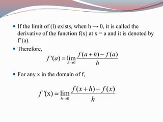
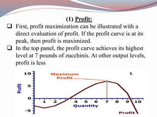
![ f’(x) is called the derivative of f(x) with respect to x.
If y= f (x), then the derivative of f is also denoted by dy /
dx or d / dx [f (x)].](https://image.slidesharecdn.com/bba-i-bm-u-3-150116235357-conversion-gate01/85/Bba-i-bm-u-3-2-differentiation-4-320.jpg)
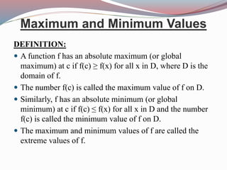
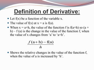
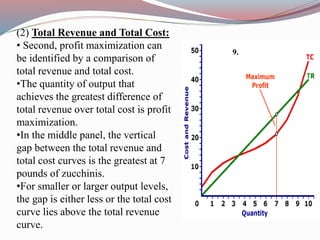
![DEFINITION:
A function f has a local maximum (or relative maximum)
at c if f(c) ≥ f(x) when x is near c.
[This means that f(c) ≥ f(x) for all x in some open interval
containing c.]
Similarly, f has a local minimum (or relative minimum) at
c if f(c) ≤ f(x) when x is near c.](https://image.slidesharecdn.com/bba-i-bm-u-3-150116235357-conversion-gate01/85/Bba-i-bm-u-3-2-differentiation-26-320.jpg)
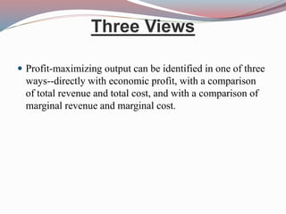


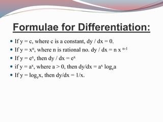
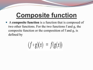
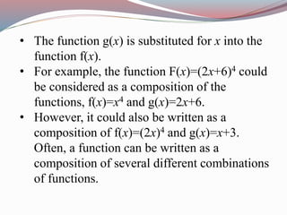
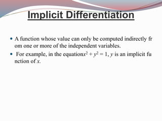
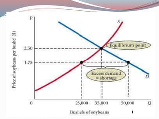
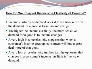
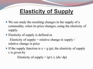
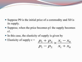
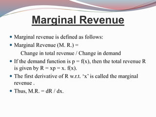
This document defines key concepts in business mathematics including derivatives, differentiation formulas, composite functions, implicit differentiation, marginal revenue, price elasticity, income elasticity, elasticity of supply, market equilibrium, cost minimization, and profit maximization. It provides formulas and explanations for each concept. Profit maximization is discussed as occurring at the level of output where marginal revenue equals marginal cost, where the difference between total revenue and total cost is highest, or at the peak of the profit curve. Cost minimization strategies include eliminating waste, simplifying processes, and negotiating better supplier prices.