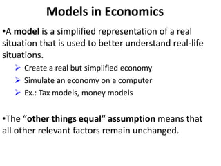
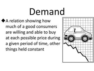
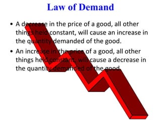
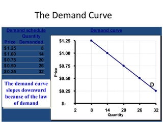
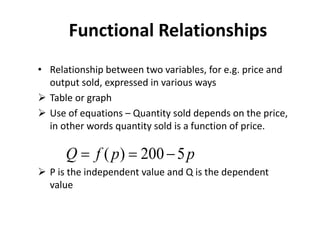
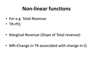
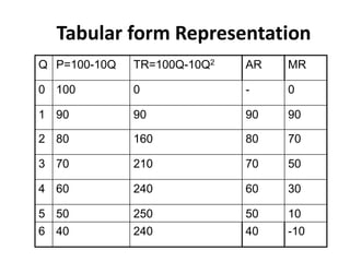
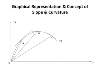
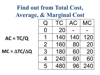
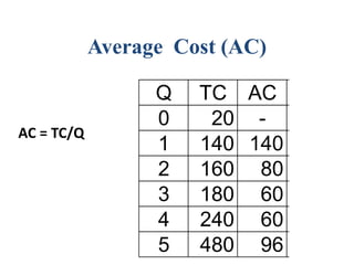
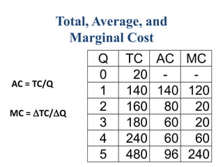
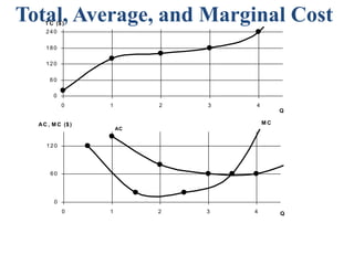
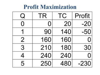
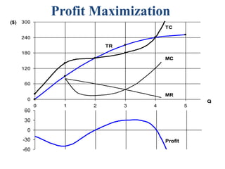
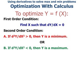
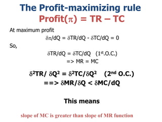
Economic Models:
Basic Mathematical Tools applied in
economics
 Simplified representations of reality play a crucial role
in economics.
Why models?
Models in Economics
•A model is a simplified representation of a real
situation that is used to better understand real-life
situations.
 Create a real but simplified economy
 Simulate an economy on a computer
 Ex.: Tax models, money models
•The “other things equal” assumption means that
all other relevant factors remain unchanged.
Demand
A relation showing how
much of a good consumers
are willing and able to buy
at each possible price during
a given period of time, other
things held constant
Law of Demand
• A decrease in the price of a good, all other
things held constant, will cause an increase in
the quantity demanded of the good.
• An increase in the price of a good, all other
things held constant, will cause a decrease in
the quantity demanded of the good.
Demand schedule Demand curve
Price
Quantity
Demanded
1.25
$ 8
1.00
$ 14
0.75
$ 20
0.50
$ 26
0.25
$ 32
$-
$0.25
$0.50
$0.75
$1.00
$1.25
2 8 14 20 26 32
Quantity
Price
D
The Demand Curve
The demand curve
slopes downward
because of the law
of demand
Functional Relationships
• Relationship between two variables, for e.g. price and
output sold, expressed in various ways
 Table or graph
 Use of equations – Quantity sold depends on the price,
in other words quantity sold is a function of price.
 P is the independent value and Q is the dependent
value
p
p
f
Q 5
200
)
( 


Linear Demand Function
QX = a0 + a1PX + a2N + a3I + a4PY + a5T
PX
QX
Intercept:
a0 + a2N + a3I + a4PY + a5T = 200
Slope:
QX/PX = a1 =-5
Non-linear functions
• For e.g. Total Revenue
• TR=PQ
• Marginal Revenue (Slope of Total revenue)
• MR=Change in TR associated with change in Q
Tabular form Representation
Q P=100-10Q TR=100Q-10Q2 AR MR
0 100 0 - 0
1 90 90 90 90
2 80 160 80 70
3 70 210 70 50
4 60 240 60 30
5 50 250 50 10
6 40 240 40 -10
Graphical Representation & Concept of
Slope & Curvature
TR
TR
Q
O
A
B
C
• Slope of TR Curve at a particular point
represents MR at a particular output, i.e.,
change in TR for an infinitesimal change in
output level
• Implication of slope for any variable implies
marginal value of the same variable
• Curvature depends on changes in slope or
changes in marginal value
Changes in Slope
Changes in Curvature
• Linear Curve – Marginal value constant, no
change in curvature
• Curve Convex to the origin – Marginal value
(Slope) changing at an increasing rate
• Curve Concave to the origin – Marginal value (
Slope) changing at a decreasing rate
Average and Marginal
• Graphically Average value can be derived from the total value
curve.
• Average at a point on the Total value curve is equal to the
slope of the ray from the origin to that particular point
• To increase (decrease) the average value, Average value
should be less (more) than the Marginal value
• Average Value constant implies its equality with Marginal
Revenue
Find out from Total Cost,
Average, & Marginal Cost
Q TC AC MC
0 20 - -
1 140 140 120
2 160 80 20
3 180 60 20
4 240 60 60
5 480 96 240
AC = TC/Q
MC = TC/Q
Average Cost (AC)
Q TC AC MC
0 20 - -
1 140 140 120
2 160 80 20
3 180 60 20
4 240 60 60
5 480 96 240
AC = TC/Q
Total, Average, and
Marginal Cost
Q TC AC MC
0 20 - -
1 140 140 120
2 160 80 20
3 180 60 20
4 240 60 60
5 480 96 240
AC = TC/Q
MC = TC/Q
Total, Average, and Marginal Cost
0
60
120
180
240
0 1 2 3 4
Q
T C ($)
0
60
120
0 1 2 3 4 Q
AC , M C ($)
AC
M C
Optimization Techniques
• In Economics different optimization techniques as a solution
to decision making problems
• Optimization implies either a variable is maximized or
minimized whichever is required for efficiency purposes,
subject to different constraints imposed on other variables
• E.g. Profit Maximization, Cost Minimization, Revenue
Maximization, Output Maximization
• A problem of maxima & minima requires the help of
differential calculus
Profit Maximization
Q TR TC Profit
0 0 20 -20
1 90 140 -50
2 160 160 0
3 210 180 30
4 240 240 0
5 250 480 -230
Profit Maximization
0
60
120
180
240
300
0 1 2 3 4 5
Q
($)
MC
MR
TC
TR
-60
-30
0
30
60
Profit
Marginal Analysis to profit maximization
• Marginal Analysis requirement for profit
Maximization,
Marginal Revenue = Marginal Cost
(MR) (MC)
• Marginal Value represents slope of Total value
curves,
• Thus slopes of TR &TC should be equal
Conditions of Profit Maximization
• MR=MC is a necessary condition for Maximization, not a
sufficient one as this condition also hold for loss maximization
• Sufficient condition requires that reaching a point of
maximization, profit should start declining with any further
rise in output, i.e. Slope of TC should rise & Slope of TR must
fall after reaching the point of Maximization,
• Change in MC>Change in MR
Concept of the Derivative
The derivative of Y with respect to X
is equal to the limit of the ratio
Y/X as X approaches zero.
Rules of Differentiation
Constant Function Rule: The derivative of a
constant, Y = f(X) = a, is zero for all values of a
(the constant).
( )
Y f X a
 
0
dY
dX

Rules of Differentiation
Power Function Rule: The derivative of
a power function, where a and b are
constants, is defined as follows.
( ) b
Y f X aX
 
1
b
dY
b aX
dX

 
Rules of Differentiation
Sum-and-Differences Rule: The derivative
of the sum or difference of two functions U
and V, is defined as follows.
( )
U g X
 ( )
V h X

dY dU dV
dX dX dX
 
Y U V
 
Rules of Differentiation
Product Rule: The derivative of the product
of two functions U and V, is defined as
follows.
( )
U g X
 ( )
V h X

dY dV dU
U V
dX dX dX
 
Y U V
 
Rules of Differentiation
Quotient Rule: The derivative of the ratio
of two functions U and V, is defined as
follows.
( )
U g X
 ( )
V h X

U
Y
V

   
2
dU dV
V U
dY dX dX
dX V


Rules of Differentiation
Logarithmic Function:
The derivative of a log function of X is defined as
follows.
d(log X)/dX= 1/X
Rules of Differentiation
Chain Rule: The derivative of a function that is a
function of X is defined as follows.
( )
U g X

( )
Y f U

dY dY dU
dX dU dX
 
Using derivatives to solve max and min problems
Optimization With Calculus
To optimize Y = f (X):
First Order Condition:
Find X such that dY/dX = 0
Second Order Condition:
A. If d2Y/dX2 > 0, then Y is a minimum.
OR
B. If d2Y/dX2 < 0, then Y is a maximum.
CENTRAL POINT
The dependent variable is maximized when its
marginal value shifts from positive to
negative, and vice versa
The Profit-maximizing rule
Profit(p) = TR – TC
At maximum profit
dp/dQ = dTR/dQ - dTC/dQ = 0
So,
dTR/dQ = dTC/dQ (1st.O.C.)
=> MR = MC
d2TR/ dQ2 = d2TC/dQ2 (2nd O.C.)
==> dMR/dQ < dMC/dQ
This means
slope of MC is greater than slope of MR function
Constrained Optimization
To optimize a function given a
single constraint, imbed the
constraint in the function and
optimize as previously defined

Mathematical Tools in Economics.pptx

  • 1.
    Economic Models: Basic MathematicalTools applied in economics
  • 2.
     Simplified representationsof reality play a crucial role in economics. Why models?
  • 3.
    Models in Economics •Amodel is a simplified representation of a real situation that is used to better understand real-life situations.  Create a real but simplified economy  Simulate an economy on a computer  Ex.: Tax models, money models •The “other things equal” assumption means that all other relevant factors remain unchanged.
  • 4.
    Demand A relation showinghow much of a good consumers are willing and able to buy at each possible price during a given period of time, other things held constant
  • 5.
    Law of Demand •A decrease in the price of a good, all other things held constant, will cause an increase in the quantity demanded of the good. • An increase in the price of a good, all other things held constant, will cause a decrease in the quantity demanded of the good.
  • 6.
    Demand schedule Demandcurve Price Quantity Demanded 1.25 $ 8 1.00 $ 14 0.75 $ 20 0.50 $ 26 0.25 $ 32 $- $0.25 $0.50 $0.75 $1.00 $1.25 2 8 14 20 26 32 Quantity Price D The Demand Curve The demand curve slopes downward because of the law of demand
  • 7.
    Functional Relationships • Relationshipbetween two variables, for e.g. price and output sold, expressed in various ways  Table or graph  Use of equations – Quantity sold depends on the price, in other words quantity sold is a function of price.  P is the independent value and Q is the dependent value p p f Q 5 200 ) (   
  • 8.
    Linear Demand Function QX= a0 + a1PX + a2N + a3I + a4PY + a5T PX QX Intercept: a0 + a2N + a3I + a4PY + a5T = 200 Slope: QX/PX = a1 =-5
  • 9.
    Non-linear functions • Fore.g. Total Revenue • TR=PQ • Marginal Revenue (Slope of Total revenue) • MR=Change in TR associated with change in Q
  • 10.
    Tabular form Representation QP=100-10Q TR=100Q-10Q2 AR MR 0 100 0 - 0 1 90 90 90 90 2 80 160 80 70 3 70 210 70 50 4 60 240 60 30 5 50 250 50 10 6 40 240 40 -10
  • 11.
    Graphical Representation &Concept of Slope & Curvature TR TR Q O A B C
  • 12.
    • Slope ofTR Curve at a particular point represents MR at a particular output, i.e., change in TR for an infinitesimal change in output level • Implication of slope for any variable implies marginal value of the same variable • Curvature depends on changes in slope or changes in marginal value Changes in Slope
  • 13.
    Changes in Curvature •Linear Curve – Marginal value constant, no change in curvature • Curve Convex to the origin – Marginal value (Slope) changing at an increasing rate • Curve Concave to the origin – Marginal value ( Slope) changing at a decreasing rate
  • 14.
    Average and Marginal •Graphically Average value can be derived from the total value curve. • Average at a point on the Total value curve is equal to the slope of the ray from the origin to that particular point • To increase (decrease) the average value, Average value should be less (more) than the Marginal value • Average Value constant implies its equality with Marginal Revenue
  • 15.
    Find out fromTotal Cost, Average, & Marginal Cost Q TC AC MC 0 20 - - 1 140 140 120 2 160 80 20 3 180 60 20 4 240 60 60 5 480 96 240 AC = TC/Q MC = TC/Q
  • 16.
    Average Cost (AC) QTC AC MC 0 20 - - 1 140 140 120 2 160 80 20 3 180 60 20 4 240 60 60 5 480 96 240 AC = TC/Q
  • 17.
    Total, Average, and MarginalCost Q TC AC MC 0 20 - - 1 140 140 120 2 160 80 20 3 180 60 20 4 240 60 60 5 480 96 240 AC = TC/Q MC = TC/Q
  • 18.
    Total, Average, andMarginal Cost 0 60 120 180 240 0 1 2 3 4 Q T C ($) 0 60 120 0 1 2 3 4 Q AC , M C ($) AC M C
  • 19.
    Optimization Techniques • InEconomics different optimization techniques as a solution to decision making problems • Optimization implies either a variable is maximized or minimized whichever is required for efficiency purposes, subject to different constraints imposed on other variables • E.g. Profit Maximization, Cost Minimization, Revenue Maximization, Output Maximization • A problem of maxima & minima requires the help of differential calculus
  • 20.
    Profit Maximization Q TRTC Profit 0 0 20 -20 1 90 140 -50 2 160 160 0 3 210 180 30 4 240 240 0 5 250 480 -230
  • 21.
    Profit Maximization 0 60 120 180 240 300 0 12 3 4 5 Q ($) MC MR TC TR -60 -30 0 30 60 Profit
  • 22.
    Marginal Analysis toprofit maximization • Marginal Analysis requirement for profit Maximization, Marginal Revenue = Marginal Cost (MR) (MC) • Marginal Value represents slope of Total value curves, • Thus slopes of TR &TC should be equal
  • 23.
    Conditions of ProfitMaximization • MR=MC is a necessary condition for Maximization, not a sufficient one as this condition also hold for loss maximization • Sufficient condition requires that reaching a point of maximization, profit should start declining with any further rise in output, i.e. Slope of TC should rise & Slope of TR must fall after reaching the point of Maximization, • Change in MC>Change in MR
  • 24.
    Concept of theDerivative The derivative of Y with respect to X is equal to the limit of the ratio Y/X as X approaches zero.
  • 25.
    Rules of Differentiation ConstantFunction Rule: The derivative of a constant, Y = f(X) = a, is zero for all values of a (the constant). ( ) Y f X a   0 dY dX 
  • 26.
    Rules of Differentiation PowerFunction Rule: The derivative of a power function, where a and b are constants, is defined as follows. ( ) b Y f X aX   1 b dY b aX dX   
  • 27.
    Rules of Differentiation Sum-and-DifferencesRule: The derivative of the sum or difference of two functions U and V, is defined as follows. ( ) U g X  ( ) V h X  dY dU dV dX dX dX   Y U V  
  • 28.
    Rules of Differentiation ProductRule: The derivative of the product of two functions U and V, is defined as follows. ( ) U g X  ( ) V h X  dY dV dU U V dX dX dX   Y U V  
  • 29.
    Rules of Differentiation QuotientRule: The derivative of the ratio of two functions U and V, is defined as follows. ( ) U g X  ( ) V h X  U Y V      2 dU dV V U dY dX dX dX V  
  • 30.
    Rules of Differentiation LogarithmicFunction: The derivative of a log function of X is defined as follows. d(log X)/dX= 1/X
  • 31.
    Rules of Differentiation ChainRule: The derivative of a function that is a function of X is defined as follows. ( ) U g X  ( ) Y f U  dY dY dU dX dU dX  
  • 32.
    Using derivatives tosolve max and min problems Optimization With Calculus To optimize Y = f (X): First Order Condition: Find X such that dY/dX = 0 Second Order Condition: A. If d2Y/dX2 > 0, then Y is a minimum. OR B. If d2Y/dX2 < 0, then Y is a maximum.
  • 33.
    CENTRAL POINT The dependentvariable is maximized when its marginal value shifts from positive to negative, and vice versa
  • 34.
    The Profit-maximizing rule Profit(p)= TR – TC At maximum profit dp/dQ = dTR/dQ - dTC/dQ = 0 So, dTR/dQ = dTC/dQ (1st.O.C.) => MR = MC d2TR/ dQ2 = d2TC/dQ2 (2nd O.C.) ==> dMR/dQ < dMC/dQ This means slope of MC is greater than slope of MR function
  • 35.
    Constrained Optimization To optimizea function given a single constraint, imbed the constraint in the function and optimize as previously defined