Naïve Bayes is a probabilistic classifier that applies Bayes' theorem with a strong (naive) independence assumption. It estimates the probability of a class given an instance by calculating the product of the prior probability of the class and the conditional probability of each attribute value given the class. This allows easy and fast training by separately estimating attribute probabilities in each class from training data. Classification is done by looking up these probabilities to find the class with the highest posterior probability for a new instance. Naïve Bayes works surprisingly well in practice despite its independence assumption often being violated.

1. Naïve Bayes Classifier
Ke Chen
http://intranet.cs.man.ac.uk/mlo/comp20411/
Modified and extended by Longin Jan Latecki
latecki@temple.edu

2. 2
Outline
• Background
• Probability Basics
• Probabilistic Classification
• Naïve Bayes
• Example: Play Tennis
• Relevant Issues
• Conclusions

3. 3
Background
• There are three methods to establish a classifier
a) Model a classification rule directly
Examples: k-NN, decision trees, perceptron, SVM
b) Model the probability of class memberships given input data
Example: multi-layered perceptron with the cross-entropy cost
c) Make a probabilistic model of data within each class
Examples: naive Bayes, model based classifiers
• a) and b) are examples of discriminative classification
• c) is an example of generative classification
• b) and c) are both examples of probabilistic classification

4. 4
Probability Basics
• Prior, conditional and joint probability
– Prior probability:
– Conditional probability:
– Joint probability:
– Relationship:
– Independence:
• Bayesian Rule
)
|
,
)
( 1
2
1 X
P(X
X
|
X
P 2
)
(
)
(
)
(
)
(
X
X
X
P
C
P
C
|
P
|
C
P 
)
(X
P
)
)
(
),
,
( 2
2 ,X
P(X
P
X
X 1
1 
 X
X
)
(
)
|
(
)
(
)
|
(
) 2
2
1
1
1
2
2 X
P
X
X
P
X
P
X
X
P
,X
P(X1 

)
(
)
(
)
),
(
)
|
(
),
(
)
|
( 2
1
2
1
2
1
2
1
2 X
P
X
P
,X
P(X
X
P
X
X
P
X
P
X
X
P 1 


Evidence
Prior
Likelihood
Posterior



5. Example by Dieter Fox

8. 8
Probabilistic Classification
• Establishing a probabilistic model for classification
– Discriminative model
– Generative model
• MAP classification rule
– MAP: Maximum A Posterior
– Assign x to c* if
• Generative classification with the MAP rule
– Apply Bayesian rule to convert:
)
,
,
,
)
( 1 n
1
L X
(X
c
,
,
c
C
|
C
P 






 X
X
)
,
,
,
)
( 1 n
1
L X
(X
c
,
,
c
C
C
|
P 






 X
X
L
c
,
,
c
c
c
c
|
c
C
P
|
c
C
P 








 1
*
*
,
)
(
)
( x
X
x
X
)
(
)
(
)
(
)
(
)
(
)
( C
P
C
|
P
P
C
P
C
|
P
|
C
P X
X
X
X 


9. Feature Histograms
x
C1
C2
P(x)
Slide by Stephen Marsland

10. Posterior Probability
x
P(C|x)
1
0
Slide by Stephen Marsland

11. 11
Naïve Bayes
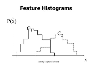
• Bayes classification
Difficulty: learning the joint probability
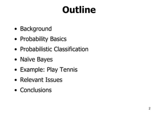
• Naïve Bayes classification
– Making the assumption that all input attributes are independent
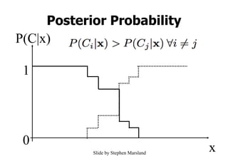
– MAP classification rule
)
(
)
|
,
,
(
)
(
)
(
)
( 1 C
P
C
X
X
P
C
P
C
|
P
|
C
P n




 X
X
)
|
,
,
( 1 C
X
X
P n



)
|
(
)
|
(
)
|
(
)
|
,
,
(
)
|
(
)
|
,
,
(
)
;
,
,
|
(
)
|
,
,
,
(
2
1
2
1
2
2
1
2
1
C
X
P
C
X
P
C
X
P
C
X
X
P
C
X
P
C
X
X
P
C
X
X
X
P
C
X
X
X
P
n
n
n
n
n


















L
n
n c
c
c
c
c
c
P
c
x
P
c
x
P
c
P
c
x
P
c
x
P ,
,
,
),
(
)]
|
(
)
|
(
[
)
(
)]
|
(
)
|
(
[ 1
*
1
*
*
*
1 












12. 12
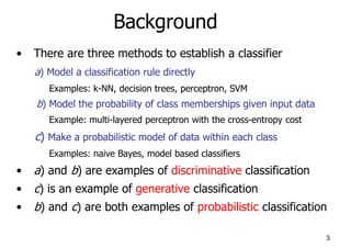
Naïve Bayes
• Naïve Bayes Algorithm (for discrete input attributes)
– Learning Phase: Given a training set S,
Output: conditional probability tables; for elements
– Test Phase: Given an unknown instance ,
Look up tables to assign the label c* to X’ if
;
in
examples
with
)
|
(
estimate
)
|
(
ˆ
)
,
1
;
,
,
1
(
attribute
each
of
value
attribute
every
For
;
in
examples
with
)
(
estimate
)
(
ˆ
of
value
target
each
For 1
S
S
i
jk
j
i
jk
j
j
j
jk
i
i
L
i
i
c
C
a
X
P
c
C
a
X
P
N
,
k
n
j
x
a
c
C
P
c
C
P
)
c
,
,
c
(c
c




















L
n
n c
c
c
c
c
c
P
c
a
P
c
a
P
c
P
c
a
P
c
a
P ,
,
,
),
(
ˆ
)]
|
(
ˆ
)
|
(
ˆ
[
)
(
ˆ
)]
|
(
ˆ
)
|
(
ˆ
[ 1
*
1
*
*
*
1 















)
,
,
( 1 n
a
a 






X
L
N
x j
j 
,

13. 13
Example
• Example: Play Tennis

14. 14
Learning Phase
Outlook Play=Yes Play=No
Sunny 2/9 3/5
Overcast 4/9 0/5
Rain 3/9 2/5
Temperature Play=Yes Play=No
Hot 2/9 2/5
Mild 4/9 2/5
Cool 3/9 1/5
Humidity Play=Yes Play=No
High 3/9 4/5
Normal 6/9 1/5
Wind Play=Yes Play=No
Strong 3/9 3/5
Weak 6/9 2/5
P(Play=Yes) = 9/14 P(Play=No) = 5/14
P(Outlook=o|Play=b) P(Temperature=t|Play=b)
P(Humidity=h|Play=b) P(Wind=w|Play=b)

15. 15
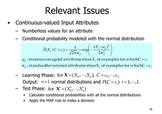
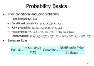
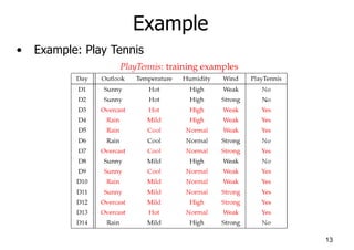
Example
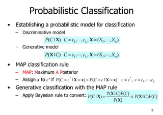
• Test Phase
– Given a new instance,
x’=(Outlook=Sunny, Temperature=Cool, Humidity=High, Wind=Strong)
– Look up tables
– MAP rule
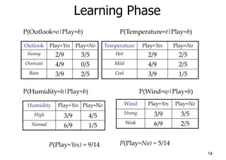
P(Outlook=Sunny|Play=No) = 3/5
P(Temperature=Cool|Play==No) = 1/5
P(Huminity=High|Play=No) = 4/5
P(Wind=Strong|Play=No) = 3/5
P(Play=No) = 5/14
P(Outlook=Sunny|Play=Yes) = 2/9
P(Temperature=Cool|Play=Yes) = 3/9
P(Huminity=High|Play=Yes) = 3/9
P(Wind=Strong|Play=Yes) = 3/9
P(Play=Yes) = 9/14
P(Yes|x’): [P(Sunny|Yes)P(Cool|Yes)P(High|Yes)P(Strong|Yes)]P(Play=Yes) = 0.0053
P(No|x’): [P(Sunny|No) P(Cool|No)P(High|No)P(Strong|No)]P(Play=No) = 0.0206
Given the fact P(Yes|x’) < P(No|x’), we label x’ to be “No”.

16. 16
Relevant Issues
• Violation of Independence Assumption
– For many real world tasks,
– Nevertheless, naïve Bayes works surprisingly well anyway!
• Zero conditional probability Problem
– If no example contains the attribute value
– In this circumstance, during test
– For a remedy, conditional probabilities estimated with Laplace
smoothing:
)
|
(
)
|
(
)
|
,
,
( 1
1 C
X
P
C
X
P
C
X
X
P n
n 






0
)
|
(
ˆ
, 


 i
jk
j
jk
j c
C
a
X
P
a
X
0
)
|
(
ˆ
)
|
(
ˆ
)
|
(
ˆ
1 





 i
n
i
jk
i c
x
P
c
a
P
c
x
P
)
1
examples,
virtual"
"
of
(number
prior
to
weight
:
)
of
values
possible
for
/
1
(usually,
estimate
prior
:
which
for
examples
training
of
number
:
C
and
which
for
examples
training
of
number
:
)
|
(
ˆ










m
m
X
t
t
p
p
c
C
n
c
a
X
n
m
n
mp
n
c
C
a
X
P
j
i
i
jk
j
c
c
i
jk
j

17. Homework
• Redo the test on Slide 15 using the formula on Slide 16
with m=1.
• Compute P(Play=Yes|x’) and P(Play=No|x’) with m=0
and with m=1 for
x’=(Outlook=Overcast, Temperature=Cool, Humidity=High, Wind=Strong)
Does the result change?
17

18. 18
Relevant Issues
• Continuous-valued Input Attributes
– Numberless values for an attribute
– Conditional probability modeled with the normal distribution
– Learning Phase:
Output: normal distributions and
– Test Phase:
• Calculate conditional probabilities with all the normal distributions
• Apply the MAP rule to make a decision
i
j
ji
i
j
ji
ji
ji
j
ji
i
j
c
C
c
X
X
c
C
X
P









 



which
for
examples
of
X
values
attribute
of
deviation
standard
:
C
which
for
examples
of
values
attribute
of
(avearage)
mean
:
2
)
(
exp
2
1
)
|
(
ˆ
2
2






L
n c
c
C
X
X ,
,
),
,
,
(
for 1
1 







X
L
n
)
,
,
(
for 1 n
X
X 






X
L
i
c
C
P i ,
,
1
)
( 





19. 19
Conclusions
• Naïve Bayes based on the independence assumption
– Training is very easy and fast; just requiring considering each
attribute in each class separately
– Test is straightforward; just looking up tables or calculating
conditional probabilities with normal distributions
• A popular generative model
– Performance competitive to most of state-of-the-art classifiers
even in presence of violating independence assumption
– Many successful applications, e.g., spam mail filtering
– Apart from classification, naïve Bayes can do more…