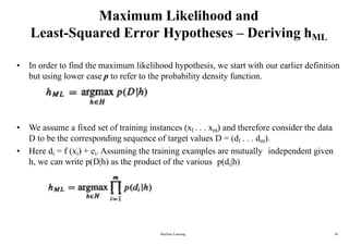
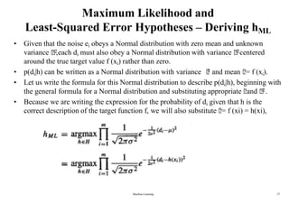
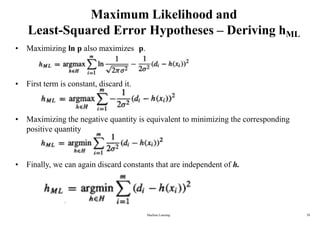
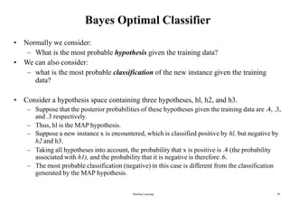
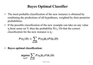
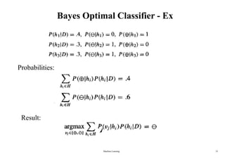
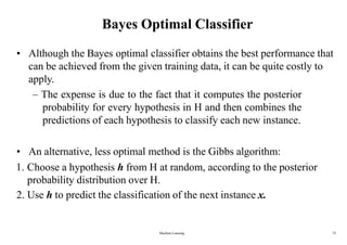
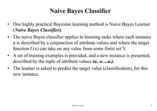
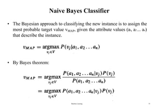
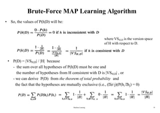
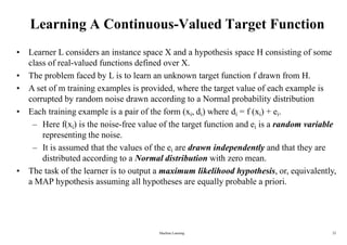
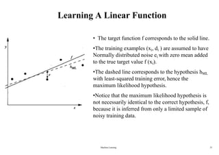
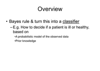
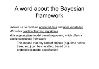
1. Bayesian learning methods are relevant to machine learning for two reasons: they provide practical classification algorithms like naive Bayes, and provide a useful perspective for understanding many learning algorithms. 2. Bayesian learning allows combining observed data with prior knowledge to determine the probability of hypotheses. It provides optimal decision making and can accommodate probabilistic predictions. 3. While Bayesian methods may require estimating probabilities and have high computational costs, they provide a standard for measuring other practical methods.

1. Introduction
Bayesian learning methods are relevant to study of machine learning for
two different reasons
• First ,Bayesian learning algorithms that calculate explicit probabilities
for hypothesis ,such as the naïve Bayes classifier ,are among the most
practical approaches to certain types of learning problems.
• The second reason is that they provide a useful perspective for
understanding many learning algorithms that do not explicitly
manipulate probabilities.

2. Overview
• Bayes rule & turn this into a classifier
–E.g. How to decide if a patient is ill or healthy,
based on
•A probabilistic model of the observed data
•Prior knowledge

3. • Training data: examples of the form (d,h(d))
– where d are the data objects to classify (inputs)
– and h(d) are the correct class info for d, h(d){1,…K}
• Goal: given dnew, provide h(dnew)
Classification problem

4. A word about the Bayesian
framework
•Allows us to combine observed data and prior knowledge
•Provides practical learning algorithms
•It is a generative (model based) approach, which offers a
useful conceptual framework
– This means that any kind of objects (e.g. time series,
trees, etc.) can be classified, based on a
probabilistic model specification

5. Bayesian Learning
Features of Bayesian learning methods:
• Each observed training example can incrementally decrease or increase the estimated
probability that a hypothesis is correct.
– This provides a more flexible approach to learning than algorithms that completely
eliminate a hypothesis if it is found to be inconsistent with any single example.
• Prior knowledge can be combined with observed data to determine the final
probability of a hypothesis. In Bayesian learning, prior knowledge is provided by
asserting
– a prior probability for each candidate hypothesis, and
– a probability distribution over observed data for each possible hypothesis.
• Bayesian methods can accommodate hypotheses that make probabilistic predictions
• New instances can be classified by combining the predictions of multiple hypotheses,
weighted by their probabilities.
• Even in cases where Bayesian methods prove computationally intractable, they can
provide a standard of optimal decision making against which other practical methods
can be measured.
Machine Learning 5

6. Machine Learning 6
Difficulties with Bayesian Methods
• Require initial knowledge of many probabilities
– When these probabilities are not known in advance they are often estimated based
on background knowledge, previously available data, and assumptions about the
form of the underlying distributions.
• Significant computational cost is required to determine the Bayes
optimal hypothesis in the general case (linear in the number of
candidate hypotheses).
– In certain specialized situations, this computational cost can be significantly
reduced.

7. Machine Learning 7
Bayes Theorem
• In machine learning, we try to determine the best hypothesis from some
hypothesis space H, given the observed training data D.
• In Bayesian learning, the best hypothesis means the most probable
hypothesis, given the data D plus any initial knowledge about the prior
probabilities of the various hypotheses in H.
• Bayes theorem provides a way to calculate the probability of a
hypothesis based on its prior probability, the probabilities of observing
various data given the hypothesis, and the observed data itself.

8. Machine Learning 8
Bayes Theorem
P(h) is prior probability of hypothesis h
– P(h) to denote the initial probability that hypothesis h holds, before observing training data.
– P(h) may reflect any background knowledge we have about the chance that h is correct. If
we have no such prior knowledge, then each candidate hypothesis might simply get the
same prior probability.
P(D) is prior probability of training data D
– The probability of D given no knowledge about which hypothesis holds
P(h|D) is posterior probability of h given D
– P(h|D) is called the posterior probability of h, because it reflects our confidence that h
holds after we have seen the training data D.
– The posterior probability P(h|D) reflects the influence of the training data D, in contrast to
the prior probability P(h), which is independent of D.
P(D|h) is posterior probability of D given h
– The probability of observing data D given some world in which hypothesis h holds.
– Generally, we write P(xly) to denote the probability of event x given event y.

9. Bayes Theorem
• In ML problems, we are interested in the probability P(h|D) that h
holds given the observed training data D.
• Bayes theorem provides a way to calculate the posterior probability
P(h|D), from the prior probability P(h), together with P(D) and P(D|h).
Bayes Theorem:
• P(h|D) increases with P(h) and P(D|h) according to Bayes theorem.
• P(h|D) decreases as P(D) increases, because the more probable it is
that D will be observed independent of h, the less evidence D provides
in support of h.
P(D)
Machine Learning 9
P(D | h) P(h)
P(h | D) =

10. Machine Learning 10
Bayes Theorem - Example
Sample Space for
events A and B
P(A) = 4/7 P(B) = 3/ 7
Is Bayes Theorem correct?
P(B|A) = 2/4 P(A|B) = 2/3
P(B|A) = P(A|B)P(B) / P(A) = ( 2/3 * 3/7 ) / 4/7 = 2/4  CORRECT
P(A|B) = P(B|A)P(A) / P(B) = ( 2/4 * 4/7 ) / 3/7 = 2/3  CORRECT
A holds T T F F T F T
B holds T F T F T F F

11. Maximum A Posteriori (MAP) Hypothesis, hMAP
• The learner considers some set of candidate hypotheses H and it is
interested in finding the most probable hypothesis h H given the
observed data D
• Any such maximally probable hypothesis is called a maximum a
posteriori (MAP) hypothesis hMAP.
• We can determine the MAP hypotheses by using Bayes theorem to
calculate the posterior probability of each candidate hypothesis.
Machine Learning 11

12. Maximum Likelihood (ML) Hypothesis, hML
• If we assume that every hypothesis in H is equally probable
i.e. P(hi) = P(hj) for all hi and hj in H
We can only consider P(D|h) to find the most probable hypothesis.
• P(D|h) is often called the likelihood of the data D given h
• Any hypothesis that maximizes P(D|h) is called a maximum likelihood
(ML) hypothesis, hML.
Machine Learning 12

13. Machine Learning 13
Example - Does patient have cancer or not?
• The test returns a correct positive result in only 98% of the cases in which the disease
is actually present, and a correct negative result in only 97% of the cases in which the
disease is not present.
• Furthermore, .008 of the entire population have cancer.
P(cancer) = .008
P(+|cancer) = .98
P(+|notcancer) = .03
P(notcancer) = .992
P(-|cancer) = .02
P(-|notcancer) = .97
• A patient takes a lab test and the result comes back positive.
P(+|cancer) P(cancer) = .98 * .008 = .0078
P(+|notcancer) P(notcancer) = .03 * .992 = .0298
• Since P(cancer|+) + P(notcancer|+) must be 1
P(cancer|+) = .0078 / (.0078+.0298) = .21
P(notcancer|+) = .0298 / (.0078+.0298) = .79
 hMAP is notcancer

14. Basic Formulas for Probabilities
Machine Learning 14

15. Machine Learning 15
Brute-Force Bayes Concept Learning
• A Concept-Learning algorithm considers a finite hypothesis space H
defined over an instance space X
• The task is to learn the target concept (a function) c : X {0,1}.
• The learner gets a set of training examples ( <x1,dl> . . . <xm,dm> )
where xi is an instance from X and di is its target value (i.e. c(xi) = di ).
• Brute-Force Bayes Concept Learning Algorithm finds the maximum a
posteriori hypothesis (hMAP), based on Bayes theorem.

16. Brute-Force MAP Learning Algorithm
• This algorithm may require significant computation, because it applies Bayes theorem
to each hypothesis in H to calculate P(h|D ) .
– While this is impractical for large hypothesis spaces,
– The algorithm is still of interest because it provides a standard against which we
may judge the performance of other concept learning algorithms.
1. For each hypothesis h in H, calculate the posterior probability
P(h|D)=
P(D|h)P(h)
P(D)
2. Output the hypothesis hMAP with the highest posterior probability
Machine Learning 16

17. Brute-Force MAP Learning Algorithm
• BF MAP learning algorithm must specify values for P(h) and P(D|h).
• P(h) and P(D|h) must be chosen to be consistent with the assumptions:
1. The training data D is noise free (i.e., di = c(xi)).
2. The target concept c is contained in the hypothesis space H
3. We have no a priori reason to believe that any hypothesis is more probable than any other.
• With these assumptions:
Machine Learning 17

18. Brute-Force MAP Learning Algorithm
• So, the values of P(h|D) will be:
• P(D) = |VSH,D| / |H| because
- the sum over all hypotheses of P(h|D) must be one and
the number of hypotheses from H consistent with D is |VSH,D| , or
- we can derive P(D) from the theorem of total probability and
the fact that the hypotheses are mutually exclusive (i.e., ( i≠ j)(P(hi hj) = 0)
where VSH,D is the version space
of H with respect to D.
Machine Learning 18

19. Evolution of posterior probabilities P(h|D)
with increasing training data.
(a) Uniform priors assign equal probability to each hypothesis.
As training data increases first to Dl (b), then to Dl D2 (c),
the posterior probability of inconsistent hypotheses becomes zero, while posterior
probabilities increase for hypotheses remaining in the version space.
Machine Learning 19

20. Machine Learning 20
MAP Hypotheses and Consistent Learners
• A learning algorithm is a consistent learner if it outputs a hypothesis that commits
zero errors over the training examples.
• Every consistent learner outputs a MAP hypothesis, if we assume
– a uniform prior probability distribution over H (i.e., P(hi) = P(hj) for all i, j), and
– deterministic, noise free training data (i.e., P(D|h) =1 if D and h are consistent, and
0 otherwise).
• Because FIND-S outputs a consistent hypothesis, it will output a MAP hypothesis
under the probability distributions P(h) and P(D|h) defined above.
• Are there other probability distributions for P(h) and P(D|h) under which FIND-S
outputs MAP hypotheses? Yes.
– Because FIND-S outputs a maximally specific hypothesis from the version space, its output
hypothesis will be a MAP hypothesis relative to any prior probability distribution that
favors more specific hypotheses.
– More precisely, suppose we have a probability distribution P(h) over H that assigns
P(h1) ≥ P(h2) if hl is more specific than h2.

21. Machine Learning 21
Maximum Likelihood and
Least-Squared Error Hypotheses
• Many learning approaches such as neural network learning, linear
regression, and polynomial curve fitting try to learn a continuous-valued
target function.
• Under certain assumptions any learning algorithm that minimizes
the squared error between the output hypothesis predictions and
the training data will output a MAXIMUM LIKELIHOOD
HYPOTHESIS.
• The significance of this result is that it provides a Bayesian justification
(under certain assumptions) for many neural network and other curve
fitting methods that attempt to minimize the sum of squared errors over
the training data.

22. Machine Learning 22
Learning A Continuous-Valued Target Function
• Learner L considers an instance space X and a hypothesis space H consisting of some
class of real-valued functions defined over X.
• The problem faced by L is to learn an unknown target function f drawn from H.
• A set of m training examples is provided, where the target value of each example is
corrupted by random noise drawn according to a Normal probability distribution
• Each training example is a pair of the form (xi, di) where di = f (xi) + ei.
– Here f(xi) is the noise-free value of the target function and ei is a random variable
representing the noise.
– It is assumed that the values of the ei are drawn independently and that they are
distributed according to a Normal distribution with zero mean.
• The task of the learner is to output a maximum likelihood hypothesis, or, equivalently,
a MAP hypothesis assuming all hypotheses are equally probable a priori.

23. Learning A Linear Function
• The target function f corresponds to the solid line.
•The training examples (xi, di ) are assumed to have
Normally distributed noise ei with zero mean added
to the true target value f (xi).
•The dashed line corresponds to the hypothesis hML
with least-squared training error, hence the
maximum likelihood hypothesis.
•Notice that the maximum likelihood hypothesis is
not necessarily identical to the correct hypothesis, f,
because it is inferred from only a limited sample of
noisy training data.
Machine Learning 23

24. Basic Concepts from Probability Theory
• Before showing why a hypothesis that minimizes the sum of squared errors in this setting is also
a maximum likelihood hypothesis, let us quickly review basic concepts from probability theory
Machine Learning 24

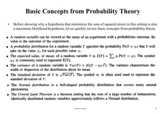
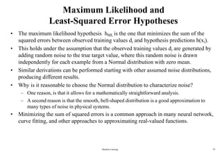
25. Basic Concepts from Probability Theory
ANormal Distribution (Gaussian Distribution)
is a bell-shaped distribution defined by the
probability density function
• ANormal distribution is fully determined by two parameters in the formula: and .
• If the random variable X follows a normal distribution:
- The probability that X will fall into the interval (a, b) is
- The expected, or mean value of X, E[X] =
- The variance of X, Var(X) = 2
- The standard deviation of X, x =
•The Central Limit Theorem states that the sum of a large number of independent, identically
distributed random variables follows a distribution that is approximately Normal.
Machine Learning 25

26. Maximum Likelihood and
Least-Squared Error Hypotheses – Deriving hML
• In order to find the maximum likelihood hypothesis, we start with our earlier definition
but using lower case p to refer to the probability density function.
• We assume a fixed set of training instances (xl . . . xm) and therefore consider the data
D to be the corresponding sequence of target values D = (dl . . . dm).
• Here di = f (xi) + ei. Assuming the training examples are mutually independent given
h, we can write p(D|h) as the product of the various p(di|h)
Machine Learning 26

27. Maximum Likelihood and
Least-Squared Error Hypotheses – Deriving hML
• Given that the noise ei obeys a Normal distribution with zero mean and unknown
variance 2
,each di must also obey a Normal distribution with variance 2centered
around the true target value f (xi) rather than zero.
• p(di|h) can be written as a Normal distribution with variance 2 and mean = f (xi).
• Let us write the formula for this Normal distribution to describe p(di|h), beginning with
the general formula for a Normal distribution and substituting appropriate and 2.
• Because we are writing the expression for the probability of di given that h is the
correct description of the target function f, we will also substitute = f (xi) = h(xi),
Machine Learning 27

28. Maximum Likelihood and
Least-Squared Error Hypotheses – Deriving hML
Machine Learning 28
• Maximizing ln p also maximizes p.
• First term is constant, discard it.
• Maximizing the negative quantity is equivalent to minimizing the corresponding
positive quantity
• Finally, we can again discard constants that are independent of h.

29. Machine Learning 29
Maximum Likelihood and
Least-Squared Error Hypotheses
• The maximum likelihood hypothesis hML is the one that minimizes the sum of the
squared errors between observed training values di and hypothesis predictions h(xi).
• This holds under the assumption that the observed training values di are generated by
adding random noise to the true target value, where this random noise is drawn
independently for each example from a Normal distribution with zero mean.
• Similar derivations can be performed starting with other assumed noise distributions,
producing different results.
• Why is it reasonable to choose the Normal distribution to characterize noise?
– One reason, is that it allows for a mathematically straightforward analysis.
– A second reason is that the smooth, bell-shaped distribution is a good approximation to
many types of noise in physical systems.
• Minimizing the sum of squared errors is a common approach in many neural network,
curve fitting, and other approaches to approximating real-valued functions.

30. Machine Learning 30
Bayes Optimal Classifier
• Normally we consider:
– What is the most probable hypothesis given the training data?
• We can also consider:
– what is the most probable classification of the new instance given the training
data?
• Consider a hypothesis space containing three hypotheses, hl, h2, and h3.
– Suppose that the posterior probabilities of these hypotheses given the training data are .4, .3,
and .3 respectively.
– Thus, hl is the MAP hypothesis.
– Suppose a new instance x is encountered, which is classified positive by hl, but negative by
h2 and h3.
– Taking all hypotheses into account, the probability that x is positive is .4 (the probability
associated with h1), and the probability that it is negative is therefore .6.
– The most probable classification (negative) in this case is different from the classification
generated by the MAP hypothesis.

31. Bayes Optimal Classifier
• The most probable classification of the new instance is obtained by
combining the predictions of all hypotheses, weighted by their posterior
probabilities.
• If the possible classification of the new example can take on any value
vj from some set V, then the probability P(vj | D) that the correct
classification for the new instance is vj :
• Bayes optimal classification:
Machine Learning 31

32. Bayes Optimal Classifier - Ex
Probabilities:
Machine Learning 32
Result:

33. Machine Learning 33
Bayes Optimal Classifier
• Although the Bayes optimal classifier obtains the best performance that
can be achieved from the given training data, it can be quite costly to
apply.
– The expense is due to the fact that it computes the posterior
probability for every hypothesis in H and then combines the
predictions of each hypothesis to classify each new instance.
• An alternative, less optimal method is the Gibbs algorithm:
1. Choose a hypothesis h from H at random, according to the posterior
probability distribution over H.
2. Use h to predict the classification of the next instance x.

34. Machine Learning 34
Naive Bayes Classifier
• One highly practical Bayesian learning method is Naive Bayes Learner
(Naive Bayes Classifier).
• The naive Bayes classifier applies to learning tasks where each instance
x is described by a conjunction of attribute values and where the target
function f (x) can take on any value from some finite set V.
• A set of training examples is provided, and a new instance is presented,
described by the tuple of attribute values (al, a2 ...an).
• The learner is asked to predict the target value (classification), for this
new instance.

35. Naive Bayes Classifier
• The Bayesian approach to classifying the new instance is to assign the
most probable target value vMAP, given the attribute values (al, a2 ... an)
that describe the instance.
• By Bayes theorem:
Machine Learning 35

36. Naive Bayes Classifier
• It is easy to estimate each of the P(vj) simply by counting the frequency with which
each target value vj occurs in the training data.
• However, estimating the different P(al,a2…an | vj) terms is not feasible unless we have
a very, very large set of training data.
– The problem is that the number of these terms is equal to the number of possible instances
times the number of possible target values.
– Therefore, we need to see every instance in the instance space many times in order to obtain
reliable estimates.
• The naive Bayes classifier is based on the simplifying assumption that the attribute
values are conditionally independent given the target value.
• For a given the target value of the instance, the probability of observing conjunction
al,a2...an, is just the product of the probabilities for the individual attributes:
• Naive Bayes classifier:
Machine Learning 36

37. Naive Bayes Classifier - Ex
CS464 IntroMduaccthioinet
L
o
e
M
a
r
a
n
c
i
n
h
g
in
e Learning
Day Outlook Temp. Humidity Wind Play Tennis
D1 Sunny Hot High Weak No
D2 Sunny Hot High Strong No
D3 Overcast Hot High Weak Yes
D4 Rain Mild High Weak Yes
D5 Rain Cool Normal Weak Yes
D6 Rain Cool Normal Strong No
D7 Overcast Cool Normal Weak Yes
D8 Sunny Mild High Weak No
D9 Sunny Cold Normal Weak Yes
D10 Rain Mild Normal Strong Yes
D11 Sunny Mild Normal Strong Yes
D12 Overcast Mild High Strong Yes
D13 Overcast Hot Normal Weak Yes
D14 Rain Mild High Strong No
33

38. Naive Bayes Classifier -Ex
• New instance to classify:
(Outlook=sunny, Temperature=cool, Humidity=high, Wind=strong)
• Our task is to predict the target value (yes or no) of the target concept
PlayTennis for this new instance.
P(Outlook=sunny|vj) P(Temperature=cool|vj)
P(Humidity=high|vj) P(Wind=strong|vj)
Machine Learning 38

39. Naive Bayes Classifier -Ex
• P(P1ayTennis = yes) = 9/14 = .64
• P(P1ayTennis = no) = 5/14 = .36
 Thus, the naive Bayes classifier assigns the target value PlayTennis = no to this new
instance, based on the probability estimates learned from the training data.
• Furthermore, by normalizing the above quantities to sum to one we can calculate the
conditional probability that the target value is no, given the observed attribute values.
.0206 / (.0206 + .0053) = .795
Machine Learning 39

40. Machine Learning 40
Estimating Probabilities
• P(Wind=strong | PlayTennis=no) by the fraction nc/n where n = 5 is the total number
of training examples for which PlayTennis=no, and nc = 3 is the number of these for
which Wind=strong.
• When nc is zero
– nc/n will be zero too
– this probability term will dominate
• To avoid this difficulty we can adopt a Bayesian approach to estimating the
probability, using the m-estimate defined as follows.
m-estimate of probability: (nc+ m*p) / (n + m)
• if an attribute has k possible values we set p = 1/k .
– p=0.5 because Wind has two possible values.
• m is called the equivalent sample size
– augmenting the n actual observations by an additional m virtual samples
distributed according to p.

41. Machine Learning 41
Learning To Classify Text
LEARN_NAIVE_BAYES_TEXT(Examples,V)
• Examples is a set of text documents along with their target values. V is
the set of all possible target values.
• This function learns the probability terms P(wk|vj), describing the
probability that a randomly drawn word from a document in class vj
will be the English word wk.
• It also learns the class prior probabilities P(vj).
1. collect all words, punctuation, and other tokens that occur in
Examples
– Vocabulary the set of all distinct words and other tokens
occurring in any text document from Examples

42. Machine Learning 42
LEARN_NAIVE_BAYES_TEXT(Examples,V)
2. calculate the required P(vj) and P(wk|vj) probability terms
For each target value vj in V do
– docsj  the subset of documents from Examples for which the
target value is vj
– P(vj)  |docsj| / |Examples|
– Textj  a single document created by concatenating all members of
docsj
– n  total number of distinct word positions in Examples
– for each word wk in Vocabulary
• nk  number of times word wk occurs in Textj
• P(wk|vj)  (nk + 1) / (n + |Vocabulary|)

43. CLASSIFY_NAIVE_BAYES_TEXT(Doc)
• Return the estimated target value for the document Doc.
• ai denotes the word found in the ith position within Doc.
– positions  all word positions in Doc that contain tokens found in
Vocabulary
– Return VNB, where
Machine Learning 43