Download to read offline

![Groundwater Flow Analysis Using Visual Modflow
DOI: 10.9790/1684-12270509 www.iosrjournals.org 9 | Page
IV. Conclusions
The study area, a part of Jakkur River Basin, Karnataka State was chosen for ground water modeling in
Visual MODFLOW Pro with the objective to understand the ground water system and to quantify the input
and output stresses.
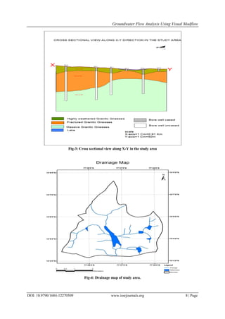
The external and internal boundaries of the model domain were demarcated. No flow, constant head and
river boundary were demarcated. Input parameters like hydraulic conductivity, storage, recharge, draft,
evapotranspiration and initial heads were assigned to the model.
The model was run both in steady state and transient flow conditions.
The model was calibrated by changing the hydraulic conductivity values by using Trial and Error Method.
The calculated vs. Observed head indicates the RMS error is 19%, 14 wells falling within the 95%
confidence interval.
Sample Hydrographs of observation wells shows the calculated heads almost ( in 50-60% of the wells)
matching the observed heads
The zone budget (recharge versus draft relationship) is obtained from the model shows at the end of stress
period 1 the ground water available is – 399 m3
/ day and at the end of stress period 12 (after 720 days) is –
49m3
/day.
Refrences
[1]. Anthony D (2002) “Preliminary surface water – groundwater interaction modelling: water balances” Technical Report No 22/02
CSIRO Land and Water Private Bag No 5 Western Australia 6913.
[2]. Bedekar. V (2011) “Abstracts of Papers & Presentations of Modflow-Surface and MODHMS” HGL Software Systems Hydro
GeoLogic, Inc.1107 Sunset Hills Road Ste. 400Reston VA 20190.
[3]. DevathaChella(2009) “Analysis of Flow Pattern between Hill and Lake” ARPN Journal of Engineering and Applied Sciences.
[4]. Elango .L (2001) “Modelling the effect of subsurface barrier on groundwater flow regime” Department of Geology,Anna
University, Chennai,Tamilnadu,India.
[5]. Fatema Akram (2012), “A Comparative View of Groundwater Flow Simulation Using Two Modelling Software - Modflow and
MIKE SHE” 18th Australasian Fluid Mechanics Conference Launceston, Australia.
[6]. Florian Werner “Groundwater Surface Water Interaction of a Post Lignite Mining Lake in Germany and its Relevance for the Local
Water Management”.
[7]. Henk M (2005) “Modeling Lake-Groundwater interactions in GFLOW”
[8]. Hoaglund(2012) “Surface-ground water interaction: From watershed process to hyporheicexchange” Kumamoto University.
[9]. Howard W (2010) “Linking MODFLOW with an Agent-Based Land-Use Model to Support Decision Making” Vol. 48, No. 5–
Ground Water (pages 649–660).
[10]. Jayaprakash. J.P (2011) “Impact Assessment and Ground Water Modelling Studies of Vented Dam at Tumbe, Dakshina Kannada
District, Karnataka” Central Ground Water Board, Bangalore.
[11]. Jay Thomas Aber (2007) “Modeling Groundwater Flow using PMWIN and ArcGIS” Water Resources Research Lab Kansas State
University.
[12]. Jairo E. Hernández1 (2012) “Modeling Groundwater Levels on the Calera Aquifer Region in Central Mexico Using ModFlow”
Journal of Agricultural Science and Technology B 2 (2012) 52-61.](https://image.slidesharecdn.com/b012270509-160711051500/85/B012270509-5-320.jpg)

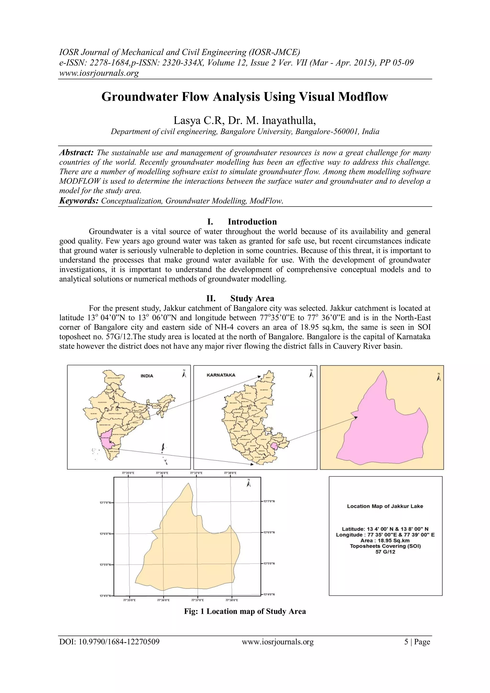
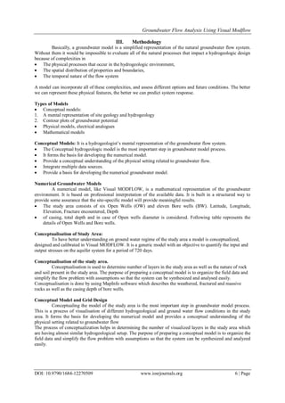
This document summarizes a study analyzing groundwater flow in the Jakkur catchment area of Bangalore, India using the Visual MODFLOW software. The study area was conceptualized as having two layers - an upper weathered and fractured layer and a lower fractured hard rock layer. Field data on open wells and borewells in the area was collected. A numerical groundwater model was developed in Visual MODFLOW using a 1km by 1km grid. The model was run in steady state and transient conditions and calibrated by adjusting hydraulic conductivity values. Sample results showed calculated heads matched observed heads in 50-60% of wells. The zone budget analysis indicated decreasing groundwater availability over time. The modeling helped quantify inputs, outputs