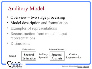
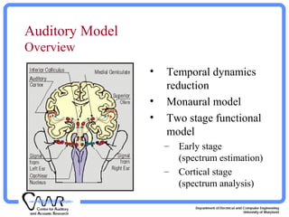
The document presents a computational auditory model detailing a two-stage processing framework for sound analysis, which includes spectrum estimation and cortical stage analysis. It describes the mathematical formulation and implementation using MATLAB, along with various auditory representations and their reconstruction from model outputs. The model aims to simulate auditory perception through a structured approach involving monaural and cortical processing stages.

1. Computational Spectro-
temporal Auditory Model
Taishih Chi
June 29, 2003

2. Auditory Model
• Overview – two stage processing
• Model description and formulation
• Examples of representations
• Reconstruction from model output
representations
• Discussions
Spectral
Estimation
Early Auditory
Spectral
Analysis
Primary Cortex (A1)
Sound
Auditory
Spectrum
Cortical
Representation

3. Auditory Model
Overview
• Temporal dynamics
reduction
• Monaural model
• Two stage functional
model
– Early stage
(spectrum estimation)
– Cortical stage
(spectrum analysis)

4. Early stage
Mathematical Formulation

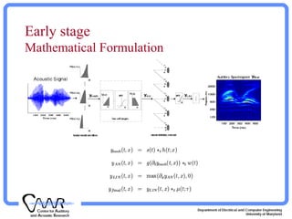
5. Early Stage MATLAB Implementation
Matlab ToolBox Usage:
yfinal = wav2aud(s, [frmlen, tc, fac, shft], filt);
s : acoustic input signal
yfinal: auditory spectrogram; N(time) x M(freq.)
CF = 440 * 2 .^ ((-31:97)/24 + shft);

6. Cortical stage
Spectrotemporal Receptive Field
4
0.125
4
0.125
4
0.125
4
0.125
4 4
0.125
C
Frequency(kHz)Frequency(kHz)
Frequency(kHz)
Frequency(kHz)
Frequency(kHz)Frequency(kHz)
Time (ms) Time (ms) Time (ms)
Time (ms) Time (ms) Time (ms)
250 250 250
250250250
0 0 0
000
0.125
D E F
BA

7. (a)
Time (ms)
Log.Frequency
Downward; Ω:1 cyc/oct, ω:4 Hz
500 1000
0.25 CF
0.5 CF
1 CF
2 CF
4 CF
(b)
-1.25 0 1.25
0
Log. Frequency (octave)
hs
0 1 2 3 4 5
0
Time (sec)
ht
Cortical stage
Model Implementation

8. Cortical stage
Mathematical Formulation
where
then the spectrotemporal cortical response:

9. Cortical stage
Mathematical Formulation (cont’d)
Consider the complex wavelet transform
where
then

10. Cortical stage
Cortical Representation of Speech
Frequency(Hz)
Time (ms)
100 200 300 400 500 600 700 800 900 1000
125
250
500
1000
2000
Multiresolution Cortical Filters and Outputs
Upward Downward
Slow Rate
Coarse Scale
Slow Rate
Fine Scale
Fast Rate
Coarse Scale
Fast Rate
Fine Scale
Slow Rate
Coarse Scale
Slow Rate
Fine Scale
Fast Rate
Coarse Scale
Fast Rate
Fine Scale

11. Cortical Magnitude Representation of Speech
Frequency(Hz)
Time (ms)
Auditory Spectrogram
100 200 300 400 500 600 700 800 900 1000
125
250
500
1000
2000
Multiresolution Cortical Filters and Outputs
Upward Downward
Slow Rate
Coarse Scale
Slow Rate
Fine Scale
Fast Rate
Coarse Scale
Fast Rate
Fine Scale
Slow Rate
Coarse Scale
Slow Rate
Fine Scale
Fast Rate
Coarse Scale
Fast Rate
Fine Scale

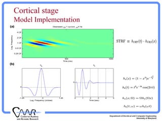
12. Cortical Stage MATLAB Implementation
Matlab ToolBox Usage:
cr = aud2cor(y, para1, rv, sv, fname, DISP);
cr: 4D cortical representation (scale-rate(up-
down)-time-freq.)
y : auditory spectrogram, N(time) x M(freq.)
para1 = [paras FULLT FULLX BP],paras:see WAV2AUD
FULLT (FULLX): fullness of temporal (spectral)
margin.
BP: pure bandpass indicator.
rv: rate vector in Hz, e.g., 2.^(1:.5:5).
sv: scale vector in cyc/oct, e.g., 2.^(-2:.5:3).