Download as PDF, PPTX

![Where we are
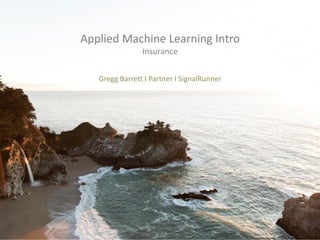
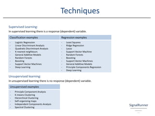
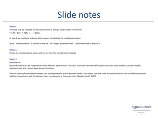
Value Proposition:
You should understand the importance of Data Science in insurance and be familiar with the
value proposition. [1]
Strategy:
The Data Science strategy covering people, process and technology is being executed.
Now:
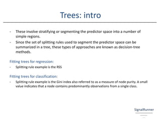
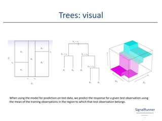
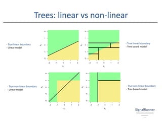
The application of a machine learning approach to classification and regression.
[1] A report on the value proposition of analytics in P&C insurance
https://1drv.ms/b/s!AnGNabcctTWNhC7AE6hW_qtJar9i](https://image.slidesharecdn.com/appliedmachinelearning-insurance-180530074437/85/Applied-machine-learning-Insurance-5-320.jpg)
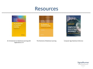
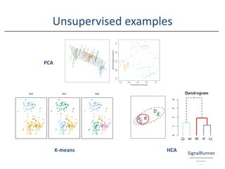
![“People learn a bunch of python and they call it a day and say, ‘Now I’m a data scientist.’ They’re not, there’s a big difference,”
“That’s what employers need to be more cognizant of. You need to hire people that have this holistic skill set that’s effective at solving
business problems.” [2]
Vasant Dhar
Professor, Stern School of Business and Center for Data Science at New York University
Founder of SCT Capital Management
[2] New Breed of Super Quants at NYU Prep for Wall Street: https://bloom.bg/2xfvN65
A reminder
The application of
modeling techniques
is not done in
isolation.](https://image.slidesharecdn.com/appliedmachinelearning-insurance-180530074437/85/Applied-machine-learning-Insurance-6-320.jpg)
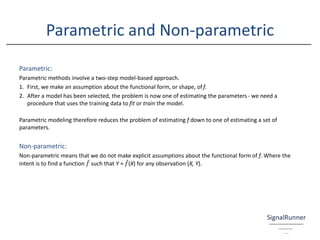
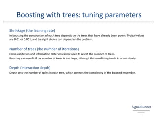
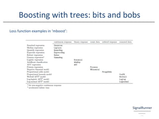
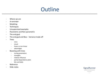
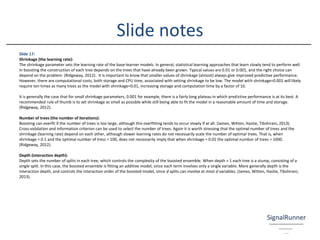
![Boosting with trees: bits and bobs
Stopping criteria for the number of trees (the number of iterations)
Various possibilities to determine the stopping iteration exist. AIC is usually not recommended as AIC-based
stopping tends to overshoot the optimal stopping dramatically. (Hofner, Mayr, Robinzonovz, Schmid, 2014)
Feature selection:
Randomised feature selection combined with backward elimination (also called recursive feature elimination)
where the least important variables are removed until out-of-bag prediction accuracy drops [3]
R Packages for boosting with trees:
XGBoost
https://cran.r-project.org/web/packages/xgboost/vignettes/xgboostPresentation.html
mboost
https://cran.r-project.org/web/packages/mboost/index.html
gbm
https://cran.r-project.org/web/packages/gbm/index.html
[3] Feature selection for ranking using boosted trees
http://bit.ly/2gukenW](https://image.slidesharecdn.com/appliedmachinelearning-insurance-180530074437/85/Applied-machine-learning-Insurance-23-320.jpg)
![Reference
Slide 5, 6:
CRISP-DM. (2000). Generic tasks (bold) and outputs (italic) of the CRISP-DM reference model. (figure). Retrieved from CRISP-DM. (2000). CRISP-DM 1.0. [pdf]. Retrieved from https://the-
modeling-agency.com/crisp-dm.pdf
Slide 8, 11, 13, 14, 27:
James, G., Witten, D., Hastie, T., Tibshirani, R. (2013). Introduction to statistical learning with applications in R. [ebook]. Retrieved from
http://www-bcf.usc.edu/~gareth/ISL/getbook.html
Slide 20:
Hastie, T., Tibshirani, R., and Friedman, J. (2009). The elements of statistical learning. data mining, inference, and prediction. Second edition. Springer Series in Statistics.
Springer. Retrieved from https://web.stanford.edu/~hastie/Papers/ESLII.pdf
Slide 21, 28:
Hofner, B., Mayr, A., Robinzonovz, N., Schmid, M. (2014). An overview on the currently implemented families in mboost. [table]. Retrieved from Hofner, B., Mayr, A., Robinzonovz, N., Schmid,
M. (2014). Model-based boosting in r: a hands-on tutorial using the r package mboost. [pdf]. Retrieved from https://cran.r-project.org/web/packages/mboost/vignettes/mboost_tutorial.pdf
Slide 22:
Hofner, B., Mayr, A., Robinzonovz, N., Schmid, M. (2014). Model-based boosting in r: a hands-on tutorial using the r package mboost. [pdf]. Retrieved from https://cran.r-
project.org/web/packages/mboost/vignettes/mboost_tutorial.pdf
Slide 25, 26:
Natekin, A., Knoll, A. (2013). Gradient boosting machines tutorial. [pdf]. Retrieved from http://www.ncbi.nlm.nih.gov/pmc/articles/PMC3885826/
Slide 26:
Yang, Y., Qian, W., Zou, H. (2014). A boosted nonparametric tweedie model for insurance premium. [pdf]. Retrieved from https://people.rit.edu/wxqsma/papers/paper4
Slide 27:
Ridgeway, G. (2012). Generalized boosted models: a guide to the gbm package. [pdf]. Retrieved from https://cran.r-project.org/web/packages/gbm/gbm.pdf
Slide 28:
Geurts, P., Irrthum, A., Wehenkel, L. (2009). Supervised learning with decision tree-based methods in computational and systems biology. [pdf]. Retrieved from
http://www.montefiore.ulg.ac.be/~geurts/Papers/geurts09-molecularbiosystems.pdf](https://image.slidesharecdn.com/appliedmachinelearning-insurance-180530074437/85/Applied-machine-learning-Insurance-24-320.jpg)

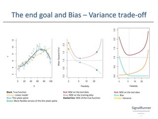
The document provides an introductory overview of the application of machine learning in insurance, emphasizing the importance of data science and various modeling techniques such as supervised and unsupervised learning. It discusses concepts like classification, regression, and the use of decision trees and boosting in modeling, along with the associated challenges such as the bias-variance trade-off. Additionally, it highlights the significance of understanding the holistic skill set required for effective data science roles in the insurance industry.


![[DSC Europe 25] Josip Saban - Career building for data professionals.pptx](https://cdn.slidesharecdn.com/ss_thumbnails/zroflcttkm1vmli0txea-josip-saban-career-building-for-data-professionals-260123083019-587cdb8c-thumbnail.jpg?width=640&height=640&fit=bounds)


![[DSC Europe 25] Milos Belcevic - Product Professional's Journey to Full-Stack...](https://cdn.slidesharecdn.com/ss_thumbnails/1zovd6fgsycdg4wvgvls-milos-belcevic-product-professionals-journey-to-full-stack-product-developer-260123083019-d993120d-thumbnail.jpg?width=640&height=640&fit=bounds)


