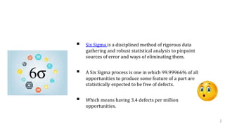
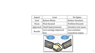
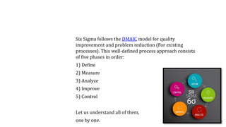
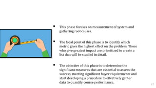
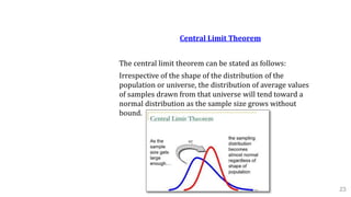
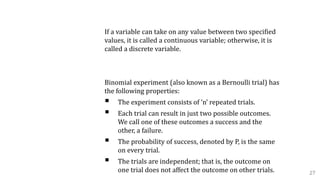
Six Sigma is a data-driven methodology for improving processes by eliminating defects. It aims for nearly flawless processes, with 99.99966% of all opportunities operating without defects. Six Sigma follows the DMAIC model, consisting of five phases - Define, Measure, Analyze, Improve, and Control. The goal is to reduce variation and maintain consistent, high-quality output through a problem-solving approach focused on addressing root causes of defects.

1. SIX SIGMASix Sigma

2. A. Introduction To Six Sigma
 Six Sigma is a disciplined method of rigorous data
gathering and robust statistical analysis to pinpoint
sources of error and ways of eliminating them.
 A Six Sigma process is one in which 99.99966% of all
opportunities to produce some feature of a part are
statistically expected to be free of defects.
 Which means having 3.4 defects per million
opportunities.
2

3. C. Lean Vs. Six Sigma
3
Aspect Lean Six Sigma
Goal Reduce Waste Reduce Variation
Focus Flow focused Problem Focused
Approach Small Improvements Variation root cause
Results
Less wastage improved
flow
Less variation
consistent output

4. B. History
It was developed by Motorola and Bill Smith in the early 1980’s
based on quality management fundamentals, and then became a
popular management approach at General Electric (GE) with Jack
Welch in the early 1990’s.
Following companies have successfully implemented Six Sigma
 Motorola
 Ericsson
 General Electric
 Sony
 Ford Motor
 CITI Bank
4

5. D. Project Selection
Approach
5
Six Sigma Process
Selection
External
Sources
Voice of
Competitor
Voice of
Customer
Voice of
Market
Internal
Sources
Voice of
Process
Voice of
Employees

6. 6

7. E. Implementation Methodology of Six Sigma
Six Sigma follows the DMAIC model for quality
improvement and problem reduction (For existing
processes). This well-defined process approach consists
of five phases in order:
1) Define
2) Measure
3) Analyze
4) Improve
5) Control
Let us understand all of them,
one by one. 7

8. 1. Define Phase
The key objectives within the Define phase are:
 Develop the Project Charter
 Define scope, objectives, and schedule
 Define the process (top-level) and its stakeholders
 Select team members
 Obtain authorization from sponsor
 Assemble and train the team
8

9. 1.1 Project Charter
Key Elements of project charter are
 Problem Statement
 Business Case
 Project scope : Constraints and Boundaries
 Team Members role
 Schedule / Milestones
 Resource Needed
9

10. Problem Statement:
 What this Project is solving in specific measureable
and quantifiable form
 How long the problem existed
 What is the impact of the problem on the company
 What is the gap between now and future
Business Case:
 Why is this worth doing? –Anticipated benefits to
customer, business and stakeholders?
 What happens if we don’t do it?
 Why now?
 What other activities have higher benefits?
 How is this project linked to organization’s strategy?
10

11. Project Scope:
 Are boundaries clear?
 Who all are impacted by this project?
 Is the scope clear and achievable in 3-6 months?
Team Members Role:
 Selection of team members
 Leader defined
 Project sponsor
 Team accountability
 Individual roles clear
11

12. Schedule / Milestones
 Timeline for DMAIC stages is defined
 Gate review between stages
 Team’s agreement and commitment
Resource Needed
 Time commitment of team members
 Management commitment to provide resources
 Who is responsible for providing resources?
12

13. 1.2 Owners and Stakeholders
 Any individual, group or institution that is affected or
is interested in the project
 The poorly managed stakeholders will have negative
effect on the project and this may lead to the project
failing
13
Interest
Power
Low Worker Management
Public CEO
HighLow
High

14. 1.3 Project Scheduling
There are a wide variety of tools and techniques available
to help the project manager develop a realistic project
timetable, to use the timetable to time the allocation of
resources, and to track progress during the
implementation of the project plan.
Following are the tools for project scheduling
 Gantt chart
 Critical Path Method (CPM)
 Program Evaluation and Review Technique (PERT)
14

15. 1.4 Team Dynamics
A team is a group of people working together towards a
common goal.
Good team shows following characteristics:
 Clarity in Team Goals
 Clearly Defined Roles
 Clear Communication
 Well Defined Decision Procedures
 Established Ground Rules
 Balanced Participation
15

16. Stages All teams go through
16
Forming
Leader Directs
Storming
Leader Coach
Norming
Leader Facilitate
Performing
Leader Delegates
Adjourning
Leader Reassure and
communicate
The forming stage
occurs when team
members first come
together as a team
During storming
stage, team
discover that
teamwork is more
difficult than they
expected
This stage begins at
completion of
storming and when
all members begins
to work as a team
When the team
reaches its high
performance stage
Breaking up of the
team, when
required task is
complete

17. 2. Measure Phase
 This phase focuses on measurement of system and
gathering root causes.
 The focal point of this phase is to identify which
metric gives the highest effect on the problem. Those
who give greatest impact are prioritized to create a
list that will be studied in detail.
 The objective of this phase is to determine the
significant measures that are essential to assess the
success, meeting significant buyer requirements and
start developing a procedure to effectively gather
data to quantify course performance.
17

18. 2.1 Statistics
Statistics convert data into information for taking action
which will help in making decisions.
18
Statistics
Descriptive
statistics
Central
Tendancy
Mean
Mode
Median
Variability
Range
Standard
Deviation
Modality
Unimodal
Bimodal
Symmetry
Symmetric
Asymmetric
Positively
Skewed
Negatively
Skiwed
Inferential
statistics

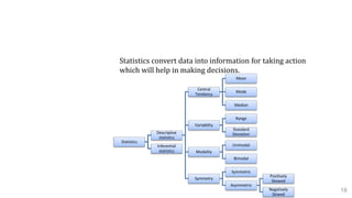
19. Descriptive statistic:
It makes use of data to provide description of the
population, either through numerical calculation or
graphs,
A. Measures of Central Tendency
Mean: Represents the sum of all values in a dataset
divided by the total number of the values. A mean score is
an average score, often denoted by X.
X = (X1 + X2 + X3 + . . . + XN) / N = [Σ Xi ] / N
Mode: The middle value in a dataset that is arranged in
ascending order
Median: Defines the most frequently occurring value in a
dataset.
19

20. B. Variability
Variability (also called spread or dispersion) refers to
how spread out a set of data is.
Range
The range is the amount between your smallest and
largest item in the set.
Range = Maximum value - Minimum value
Variance
A small number for the variance means your data set is
tightly clustered together and a large number means the
values are more spread apart.
20

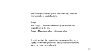
21. B. Variability
Standard Deviation:
The standard deviation tells you how tightly your data is
clustered around the mean (the average).
The standard deviation is a numerical value used to
indicate how widely individuals in a group vary.
σ = sqrt [Σ (Xi - X) 2 / N]
Where σ is the population standard deviation,
X is the population mean,
Xi is the I th element from the population
N is the number of elements in the population. 21

22. C. Modality
Unimodal: when a set of
data has only single mode
showing a single pick of
data, it is called as unimodal
D. Symmetry
Symmetry is an attribute
used to describe the shape
of a data distribution. When
it is graphed, a symmetric
distribution can be divided
at the center so that each
half is a mirror image of the
other.
22

23. 2.2 Central Limit Theorem
The central limit theorem can be stated as follows:
Irrespective of the shape of the distribution of the
population or universe, the distribution of average values
of samples drawn from that universe will tend toward a
normal distribution as the sample size grows without
bound.
23

24. 2.3 Levels of Data Measurements
24
Data
Nominal Ordinal Interval Ratio

25. 3. Analyze Phase
 This is where the statistical study of a problem starts.
 In this phase statistical reviews are done to the
groups of deviation or variation in order for project
owners to identify which are the considerable
contributors to the output.
 The focal point of this phase is to identify and
analyze the root cause/s of imperfection.
25

26. 3.1 Probability Distributions
A probability distribution is a table or an equation that
links each outcome of a statistical experiment with its
probability of occurrence.
26
Probability
Distributions
Continuous
Variables
Normal
Distribution
Discrete
Variables
Binomial
Distribution
Poisson’s
Distribution

27. Continuous Variable vs. Discrete Variable
If a variable can take on any value between two specified
values, it is called a continuous variable; otherwise, it is
called a discrete variable.
A. Binomial Distribution:
Binomial experiment (also known as a Bernoulli trial) has
the following properties:
 The experiment consists of ‘n’ repeated trials.
 Each trial can result in just two possible outcomes.
We call one of these outcomes a success and the
other, a failure.
 The probability of success, denoted by P, is the same
on every trial.
 The trials are independent; that is, the outcome on
one trial does not affect the outcome on other trials. 27

28. B. Poisson distribution
A Poisson experiment has the following properties:
 The experiment results in outcomes that can be
classified as successes or failures.
 The average number of successes (μ) that occurs in a
specified region is known.
 Outcomes are random. Occurrence of one outcome
does not influence the chance of another outcome of
interest.
 The outcomes of interest are rare relative to the
possible outcomes.
28

29. C. Normal Probability Distribution
Normal Distribution has following Characteristics:
 About 68% of the area under the curve falls within 1
standard deviation of the mean.
 About 95% of the area under the curve falls within 2
standard deviations of the mean.
 About 99.7% of the area under the curve falls within
3 standard deviations of the mean.
 The total area under the normal curve = 1.
 The probability of any particular value is 0.
 The probability that X is greater than or less than a
value = area under the normal curve in that direction.
29

30. 3.2 Process Capability
Why to do Process Capability study?
 Understand the behaviors of new/repaired/ adjusted
equipment
 Review of tolerances
 Allocation of equipment
 The ability of the process to meet the required
specifications
Remember Following Notations:
LSL: Lower Specification limit USL: Upper Specification
limit
LCL: Lower Control limit UCL: Upper Control Limit
Cp = Capability index Cpk = Performance index
𝞼 = Standard Deviation. µ= Mean
30

31. ◎
31

32. 3.3 Correlation and Regression
Correlation
Correlation coefficients measure the strength of association between
two variables.
 The value of a correlation coefficient ranges between -1 and 1.
 The greater the absolute value of a correlation coefficient, the
stronger the linear relationship.
 The strongest linear relationship is indicated by a correlation
coefficient of -1 or 1.
 The weakest linear relationship is indicated by a correlation
coefficient equal to 0.
32

33. 3.4 Hypothesis Testing
Hypothesis is a claim, which we have to test.
Null Hypothesis -H0
Default position / currently accepted position / Assumed /
Status
Alternate Hypothesis –Ha
Claim to be tested. Also known as Research Hypothesis or
the other option.
You either reject the null hypothesis or fail to reject. You
never accept Null Hypothesis.
If Null Hypothesis is rejected you proceed to Alternate
Hypothesis. 33

34. 3.4 Hypothesis Testing
Level of Confidence (C):
In most of the cases, if nothing is given we prefer to have
95%
Shows a % of chance when you can wrongly reject the null
hypothesis
Level of Significance α: 1-C,
Types of Errors
34

35. 4. Improve Phase
 The objective of Improve Phase is to identify
improvement breakthroughs, identify high gain
alternatives, select preferred approach, design the
future state.
4.1 Design of Experiments
 The goal is to obtain maximum information with the
minimum number of experiments
 Design of experiments (DOE) is a systematic
method to determine the relationship between
factors affecting a process and the output of that
process.
 In other words, it is used to find cause-and-effect
relationships.
35

36. 4.1 Design of Experiments
What is so special about experiments?
 Experiments allow us to set up a direct comparison
between the treatments of interest.
 We can design experiments to minimize any bias in the
comparison.
 We can design experiments so that the error in the
comparison is small.
 Most important, we are in control of experiments, and
having that control allows us to make stronger
inferences about the nature of differences that we see in
the experiment.
36

37. 5. Control Phase
The main objectives of the Control/Verify stage are to:
 Statistically validate that the new process or design
meets the objectives and benefits sought through the
project
 Develop and implement a control plan to
institutionalize the new process or Design
 Document lessons learned and project findings
37

38. 5.1 Control Chart Tree
38

39. 5.2 Interpreting control charts
39

40. 5.4 Interpreting control charts
40

41. Case Study on Mumbai Dabbawala’s
41