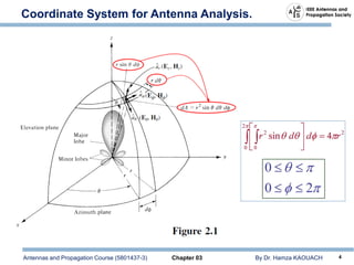
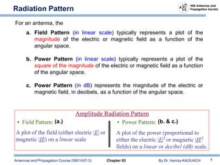
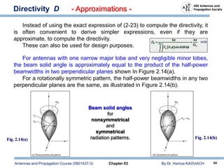
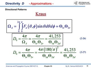
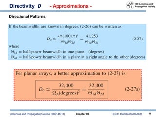
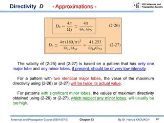
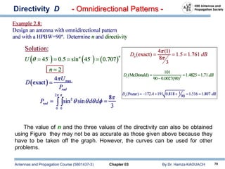
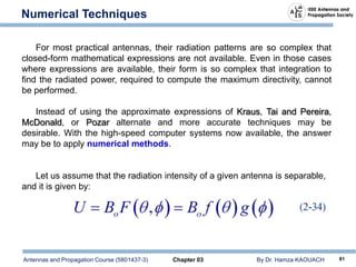
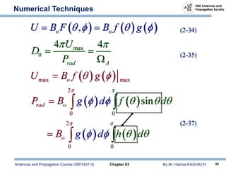
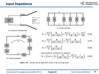
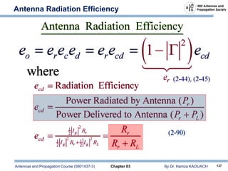
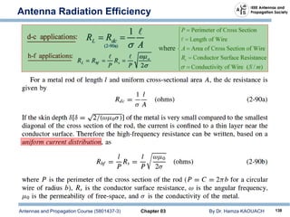
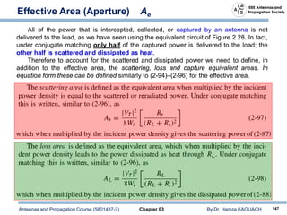
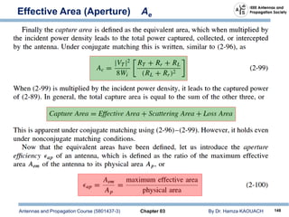
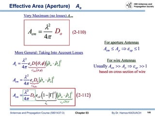
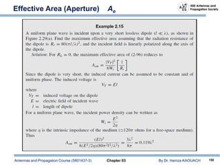
Chapter 3 of Dr. Hamza Kaouach's course on antennas and propagation discusses fundamental parameters needed to describe antenna performance, including radiation patterns, directivity, gain, and efficiency. It covers key concepts such as isotropic and directional patterns, beamwidths, and field regions around antennas, providing definitions and interrelations among these parameters. The chapter also references IEEE standards for definitions and emphasizes the importance of the radiation pattern and its components in characterizing antenna behavior.
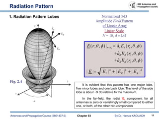
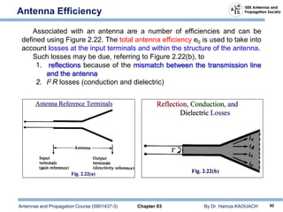


![Antenna lecture course CHapter 2_(2)[1].pdf](https://cdn.slidesharecdn.com/ss_thumbnails/antennach221-240525095938-532f47be-thumbnail.jpg?width=640&height=640&fit=bounds)