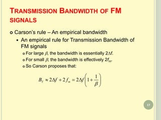
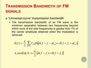
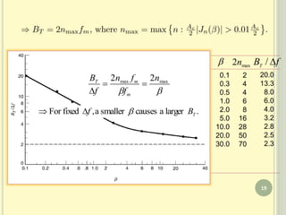
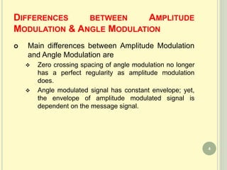
This document discusses angle modulation techniques. It defines angle modulation as varying the angle of the carrier signal in accordance with the baseband signal. The key types of angle modulation are phase modulation and frequency modulation. Frequency modulation provides better noise performance than amplitude modulation at the cost of increased bandwidth. Narrowband FM is approximated using Bessel functions. Carson's rule and the universal bandwidth curve describe how the transmission bandwidth of FM signals depends on the modulation index.

1. ANGLE MODULATION
BY
G.GNANA PRIYA
AP/ECE
RAMCO INSTITUTE OF
TECHNOLOGY

2. 2
ANGLE MODULATION
 Definition
 The angle of the carrier is varied in accordance with the
baseband signal.
 Angle modulation provides us with a practical
means of exchanging channel bandwidth for
improved noise performance.
 So, angle modulation can provide better discrimination
against noise and interference than the amplitude
modulation, at the expense of increased transmission
bandwidth.

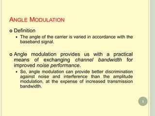
3. ANGLE MODULATION
 Commonly used angle modulation :
 Phase modulation (PM)
 Frequency modulation (FM)
y.sensitivitphaseiswhere)],(2cos[)( ppcc ktmktfAts  
 
 
y.sensitivitfrequencyisrewhe
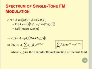
,)(22cos
))((2cos)(
0
0
f
t
fcc
t
fcc
k
dmktfA
dmkfAts






3

4. DIFFERENCES BETWEEN AMPLITUDE
MODULATION & ANGLE MODULATION
 Main differences between Amplitude Modulation
and Angle Modulation are
 Zero crossing spacing of angle modulation no longer
has a perfect regularity as amplitude modulation
does.
 Angle modulated signal has constant envelope; yet,
the envelope of amplitude modulated signal is
dependent on the message signal.
4

5. SIMILARITY BETWEEN PM AND FM
 Similarity between PM and FM is
 PM is simply an FM with in place of m(t).

t
dm
0
)( 



  
t
fccFM dmktfAts
0
)(22cos)( 
)](2cos[)( tmktfAts pccPM  
5

6. FREQUENCY MODULATION (FM)
 s(t) of FM modulation is a non-linear function of
m(t).
 So its general analysis is hard.
 To simplify the analysis, we may assume a single-
tone transmission, where
)2cos()( tfAtm mm 



 



 






t
fcc
t
fcc
t
ic
dmktfA
dmkfAdfAts
0
00
)(22cos
))((2cos)(2cos)(


6

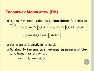
7. From the formula in the previous slide,
deviation.frequencytheiswhere
)2cos(
)2cos(
)()(
mf
mc
mmfc
fci
Akf
tfff
tfAkf
tmkftf











 




 






)2sin(2cos
)]2cos([2cos
)(2cos)(
0
0
tf
f
f
tfA
dfffA
dfAts
m
m
cc
t
mcc
t
ic



signal.FMof
indexmodulationthecalledoftenis/where mff
7

8.  Modulation index  is the largest deviation from 2fct
in FM system.
 As a result,
1. A small  corresponds to a narrowband FM.
2. A large  corresponds to a wideband FM.
 )2sin(2cos)( tftfAts mcc  
mccmcicmc fffftffftfffff   )2cos()(
8

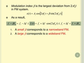
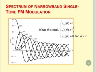
9. NARROWBAND FREQUENCY MODULATION
 
)2sin()2sin()2cos(
)]2sin(sin[)2sin()]2sin(cos[)2cos(
)2sin(2cos)(
tftfAtfA
tftfAtftfA
tftfAts
mcccc
mccmcc
mcc






(Often,  < 0.3.)
9

10. NARROWBAND FREQUENCY MODULATION
 Comparison between approximate narrowband FM
modulation and AM (DSB-C) modulation
))(2cos(
2
))(2cos(
2
)2cos(
)2cos()]2cos(1[
)2cos()](1[)(
tff
Ak
tff
Ak
tfA
tftfAkA
tftmkAts
m
ma
m
ma
cc
cmmac
cacAM






))(2cos(
2
))(2cos(
2
)2cos(
)2sin()2sin()2cos()(
tff
A
tff
A
tfA
tftfAtfAts
mc
c
mc
c
cc
mccccFM








10

11. NARROWBAND FREQUENCY MODULATION
 Represent them in terms of their low-pass
isomorphism.
)]2sin()2[cos(
2
)]2sin()2[cos(
2
)0()(~
tfjtf
Ak
tfjtf
Ak
jAts
mm
ma
mm
ma
cAM




)]2sin()2[cos(
2
)]2sin()2[cos(
2
)0()(~
tfjtf
A
tfjtf
A
jAts
mm
c
mm
c
cFM






11

12. NARROWBAND FREQUENCY MODULATION
 Phasor diagram
)]2sin()2[cos(
2
tfjtf
A
mm
c



)0( jAc 
))2sin(
)2(cos(
2
tfj
tf
A
m
m
c




)(~ tsFM
)]2sin()2[cos(
2
tfjtf
A
mm
c



)(~ tsAM
.Let mac AkA 
12

13. SPECTRUM OF SINGLE-TONE FM
MODULATION
 
   
 )2exp()(~Re
)2sin(2expRe
)2sin(2cos)(
tfjts
tftfjA
tftfAts
c
mcc
mcc






  )2sin(exp)(~ tfjAts mc 




n
ntfj
nc
m
eJAts 
 2
)()(~ )sin(
)(  jx
n
jn
n eexJ 


kind.firsttheoffunctionelorder Bessnththeis)(where nJ
13

14. SPECTRUM OF SINGLE-TONE FM
MODULATION

 
 


























n
mnc
n
tnffj
nc
ftj
n
ntfj
nc
ftj
nffJA
dteJA
dteeJA
dtetsfS
m
m
)()(
)(
)(
)(~)(
~
)(2
22
2






14

15. SPECTRUM OF SINGLE-TONE FM
MODULATION
 
 
 








n
mcmcn
c
n
mcmcn
c
cc
nfffnfffJ
A
nfffnfffJ
A
ffSffSfS
)()()(
2
)()()(
2
)(
~
)(
~
2
1
)( *


Consequently,
15

16. SPECTRUM OF NARROWBAND SINGLE-
TONE FM MODULATION
.
2for0)(
2
)(
1)(
small,isWhen 1
0










nJ
J
J
n 




16

17. TRANSMISSION BANDWIDTH OF FM
SIGNALS
 Carson’s rule – An empirical bandwidth
 An empirical rule for Transmission Bandwidth of
FM signals
 For large , the bandwidth is essentially 2f.
 For small , the bandwidth is effectively 2fm.
 So Carson proposes that:








1
1222 fffB mT
17

18. TRANSMISSION BANDWIDTH OF FM
SIGNALS
 “Universal-curve” transmission bandwidth
 The transmission bandwidth of an FM wave is the
minimum separation between two frequencies beyond
which none of the side frequencies is greater than 1% of
the carrier amplitude obtained when the modulation is
removed.
 



n
mcmcn
c
nfffnfffJ
A
fS )()()(
2
)( 
 )()(
2
)2cos( cc
c
cc ffff
A
tfA  
18

19. 0.1
0.3
0.5
1.0
2.0
5.0
10.0
20.0
30.0
2
4
4
6
8
16
28
50
70
 max2n

maxmax 22 n
f
fn
f
B
m
mT


.largeracausessmallera,fixedFor TBf 
20.0
13.3
8.0
6.0
4.0
3.2
2.8
2.5
2.3
fBT /
19

20. Thank You
20