Download to read offline
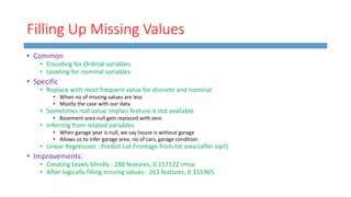

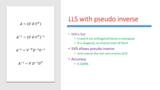
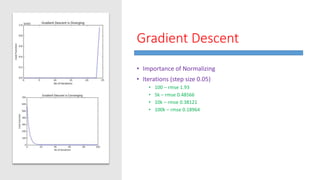
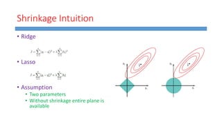
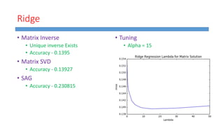
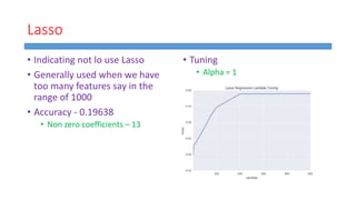
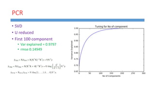
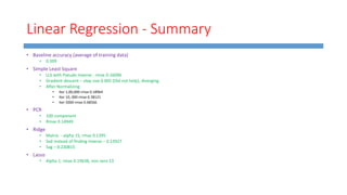
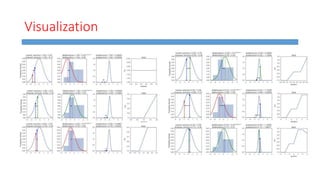
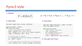
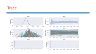
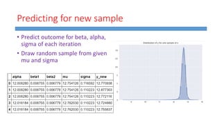
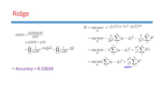
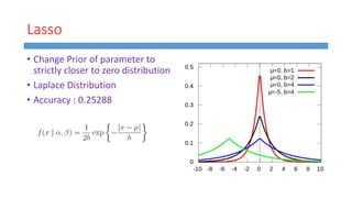
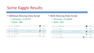


This document summarizes work done on predicting house prices using linear and Bayesian regression models on the Ames housing dataset. It describes data preprocessing like filling missing values, error metrics used, various linear regression techniques tested including least squares, gradient descent, ridge regression, lasso, and PCR. It also covers Bayesian regression using Markov chain Monte Carlo and Metropolis-Hastings sampling to estimate posterior distributions. Visualizations are shown and kaggle results are reported, with the best linear model achieving a RMSE of 0.12664 and Bayesian regression models achieving accuracies of 0.12727 and 0.33020 for ridge and 0.25288 for lasso.


![[DSC Europe 25] Ekaterina Bubenko - Behind the Curtain: How Data Roles Collab...](https://cdn.slidesharecdn.com/ss_thumbnails/anmv6x8dstqbbzchoklr-ekaterina-bubenko-behind-the-curtain-how-data-roles-collaborate-in-the-ai-era-a-260123083019-4b252ec7-thumbnail.jpg?width=640&height=640&fit=bounds)


