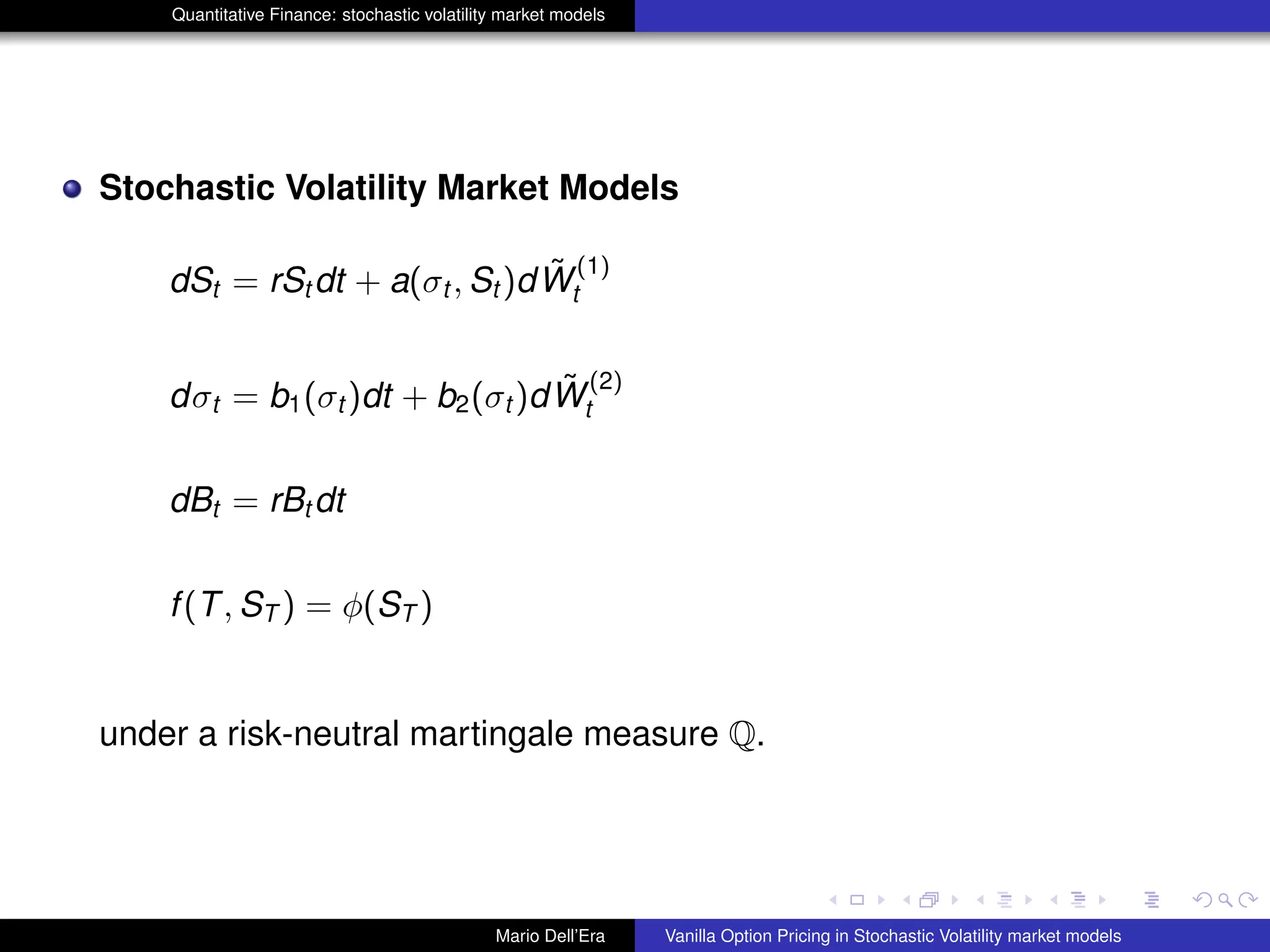
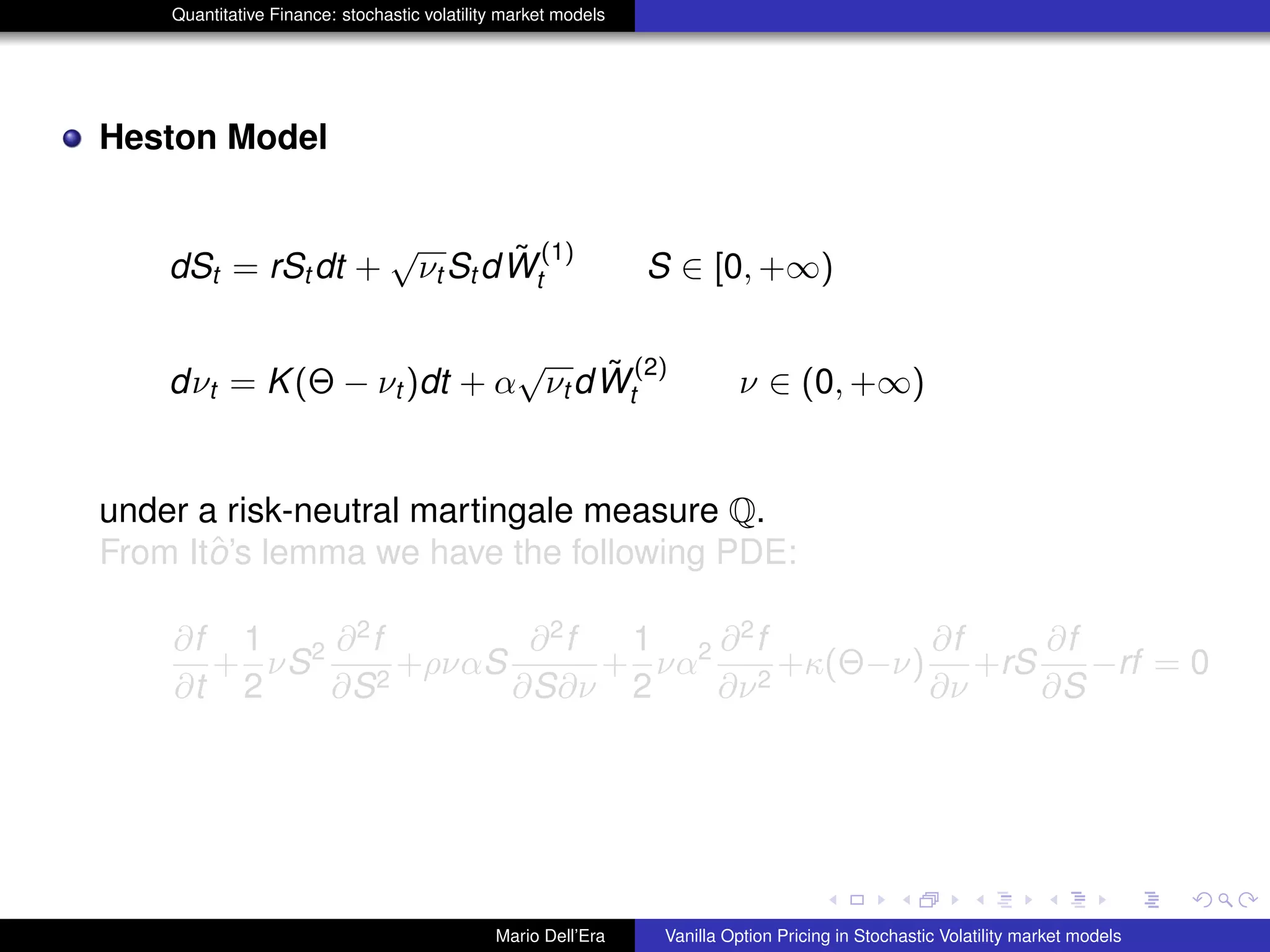
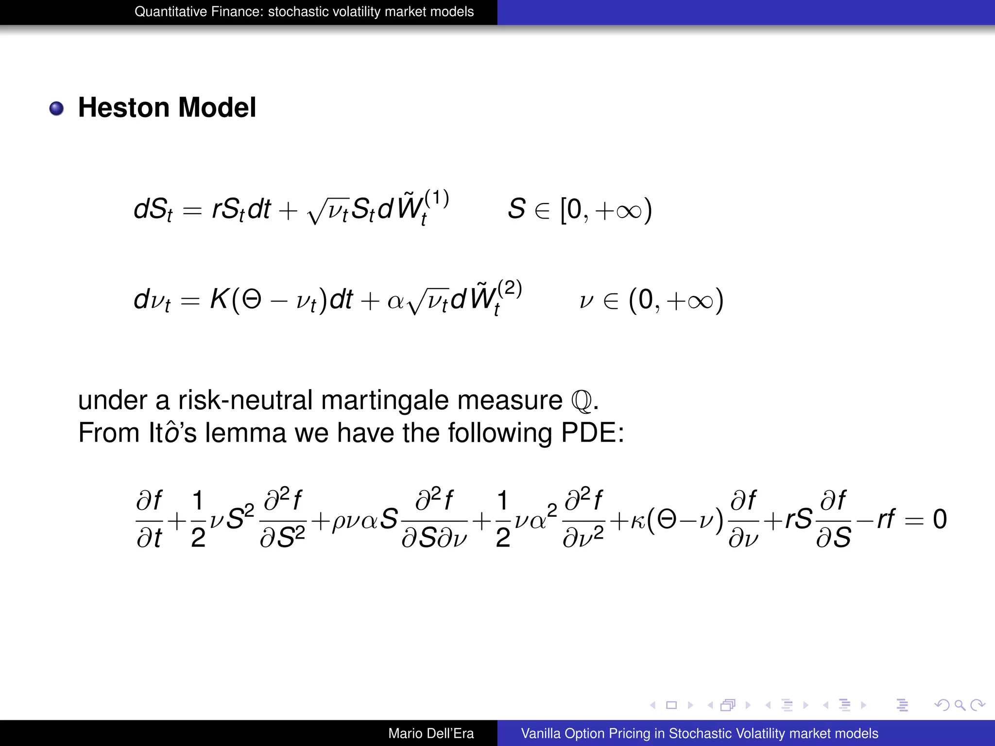
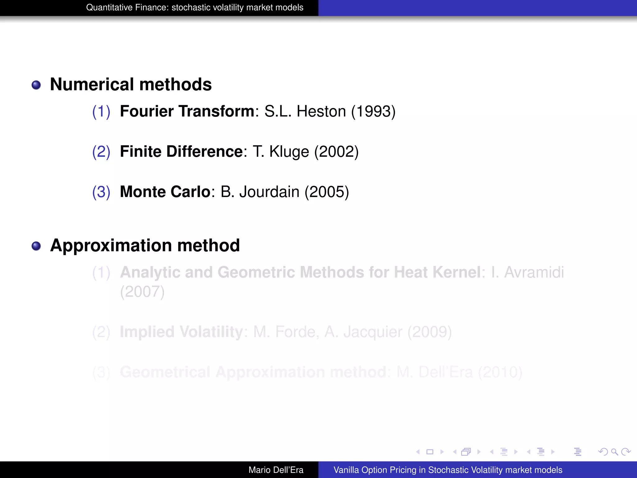
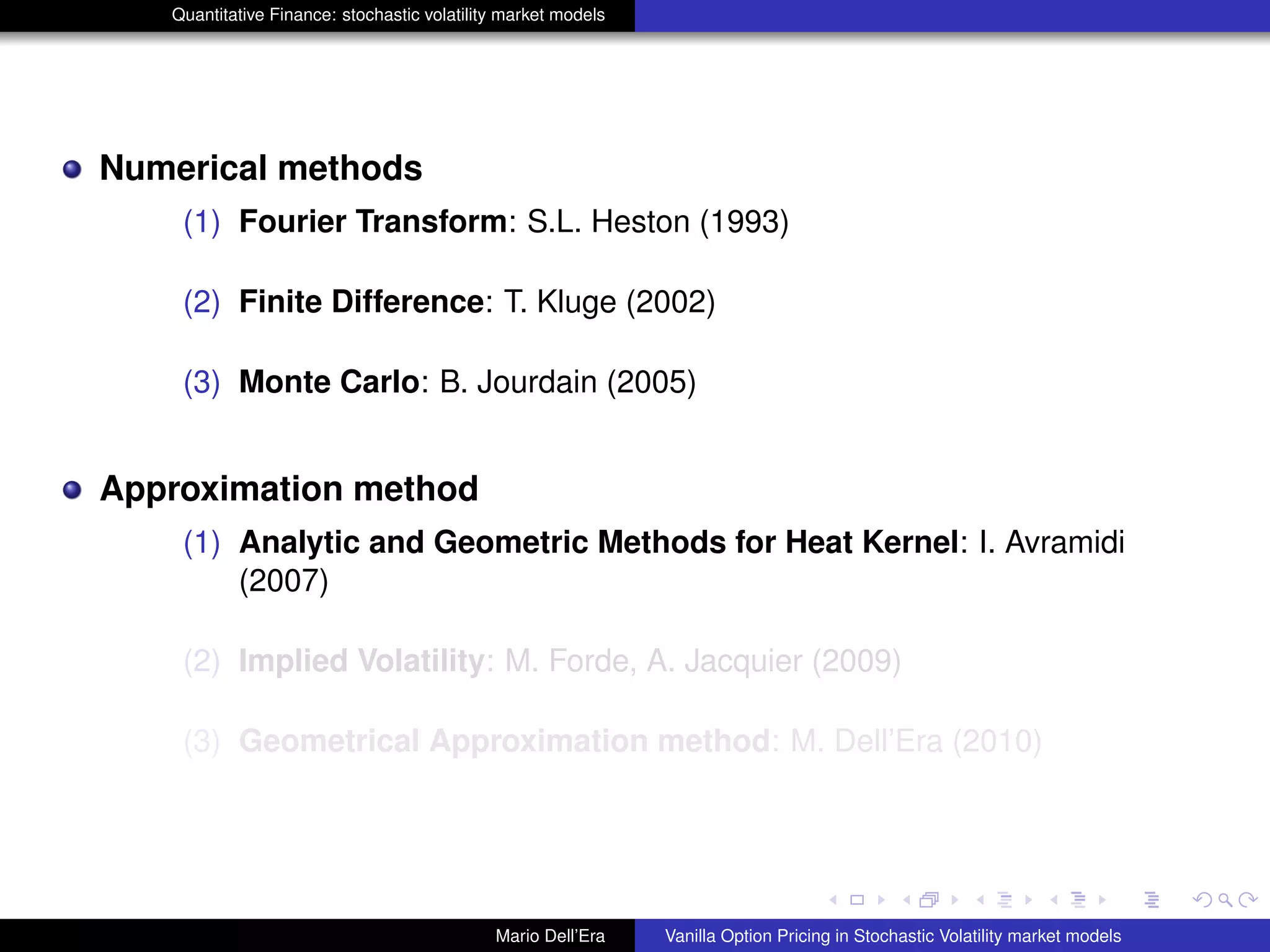
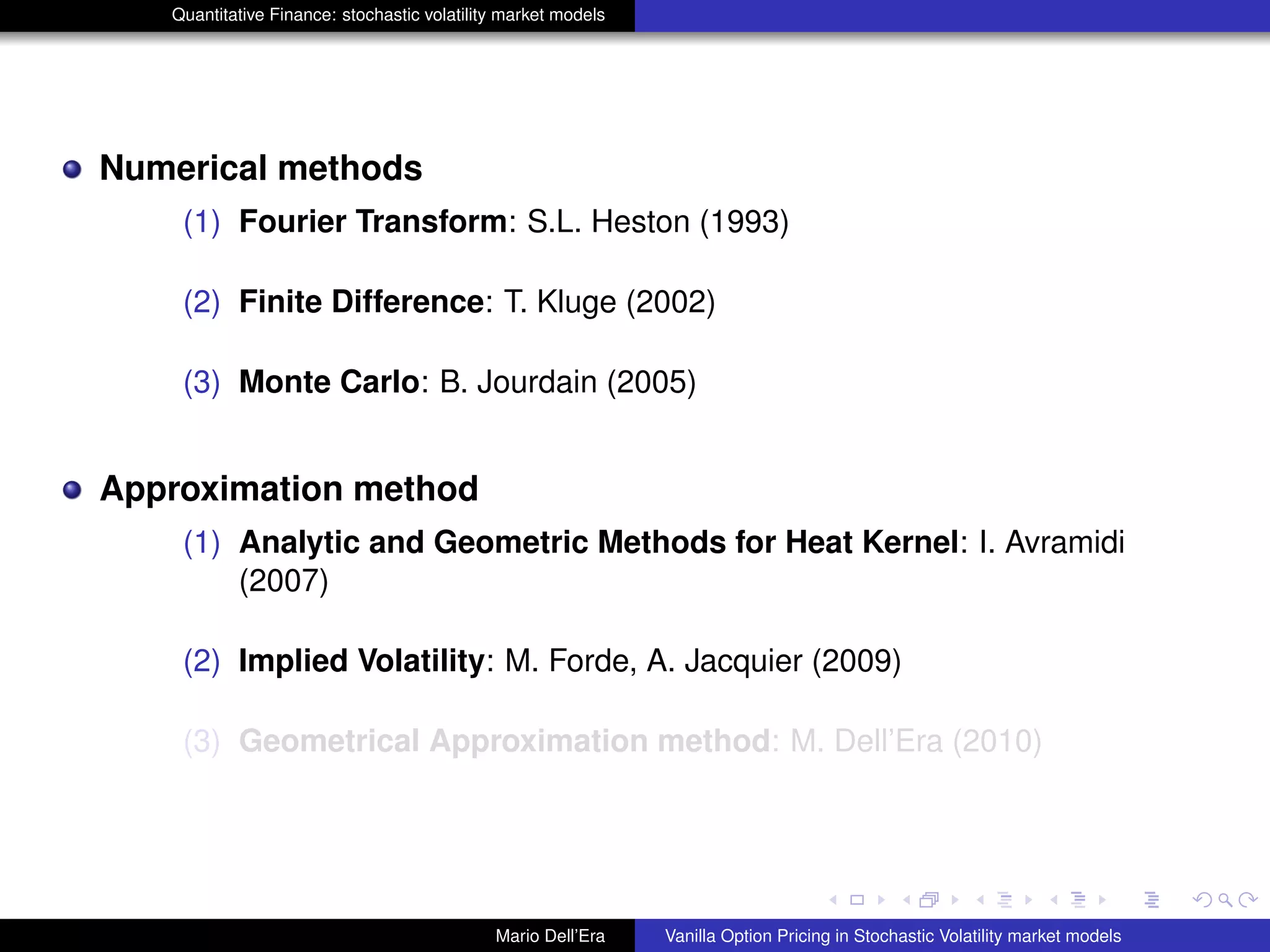
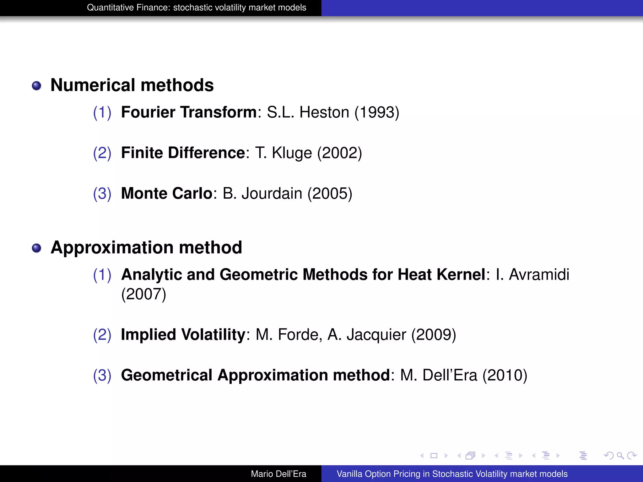
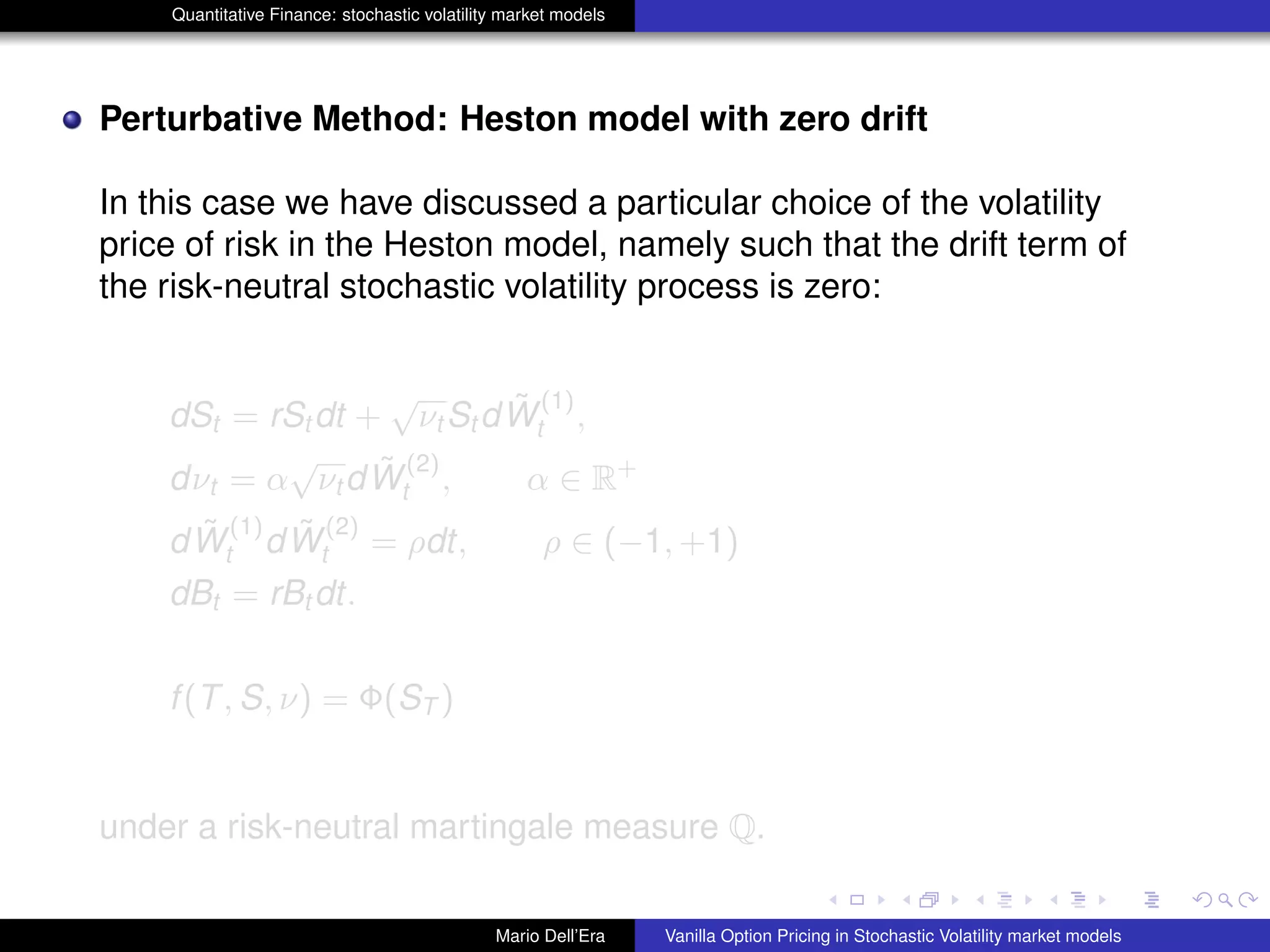
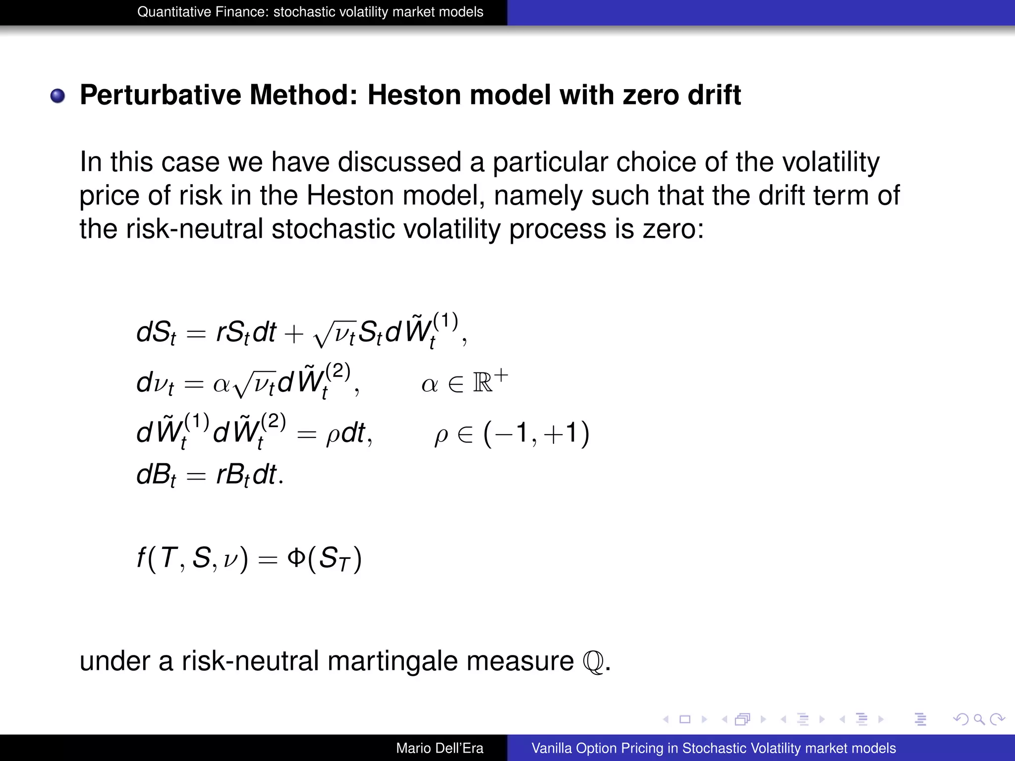
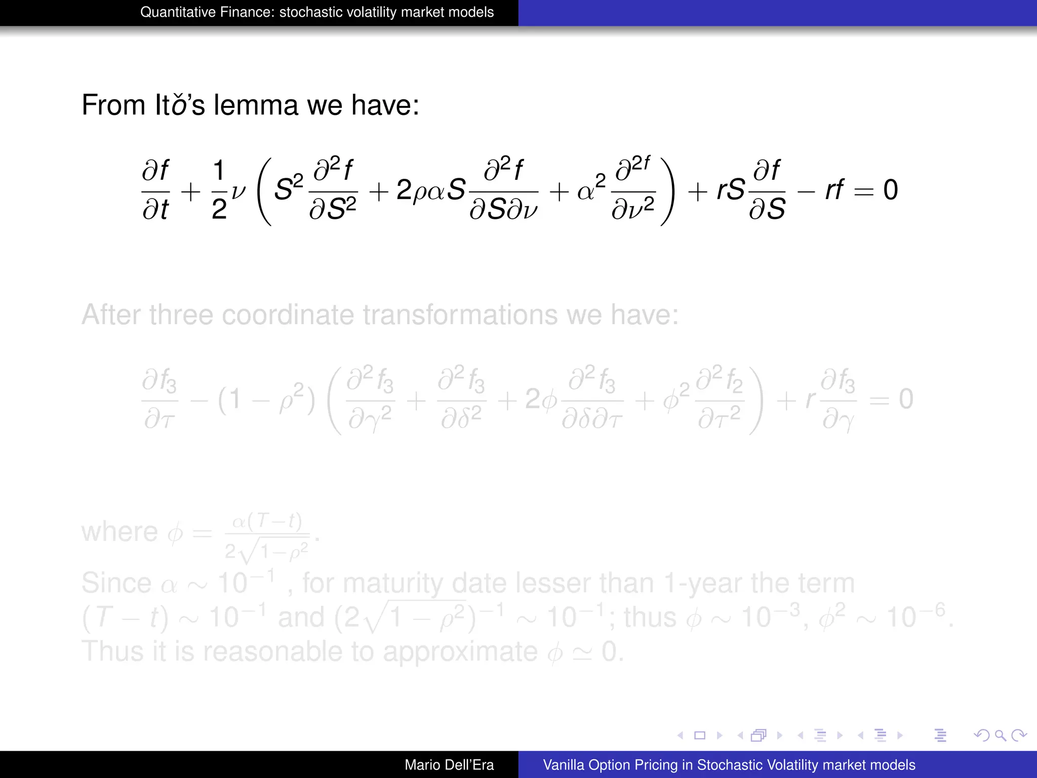
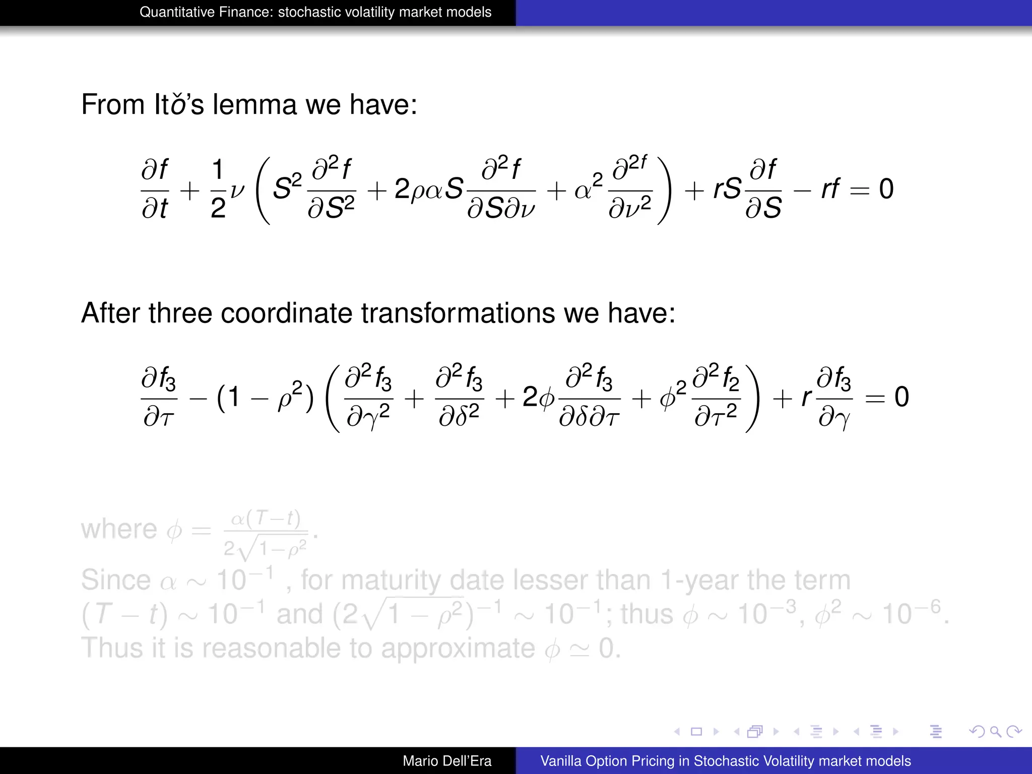
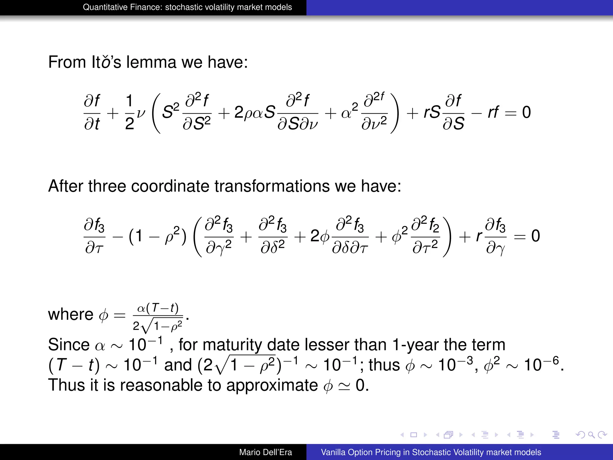
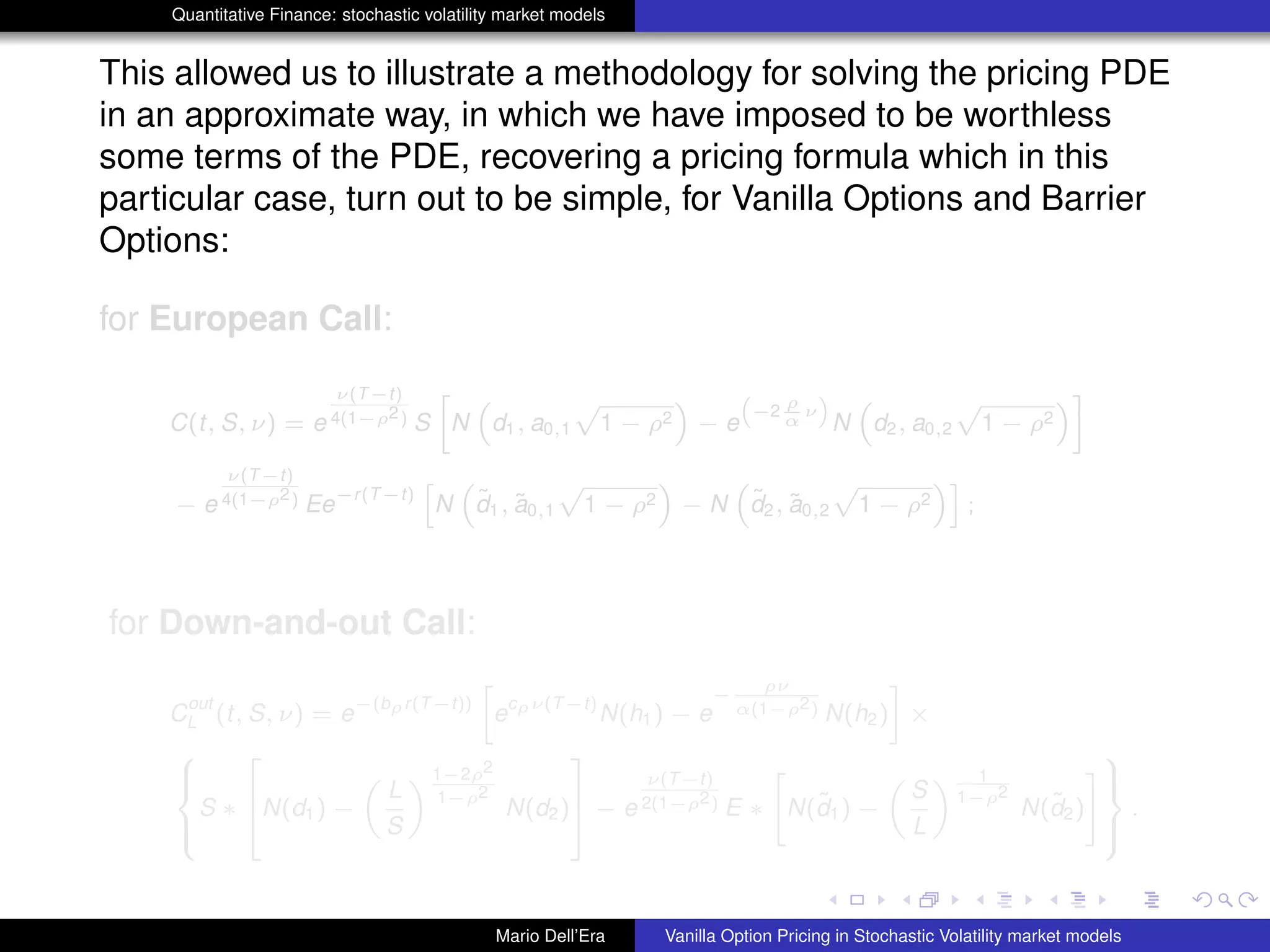
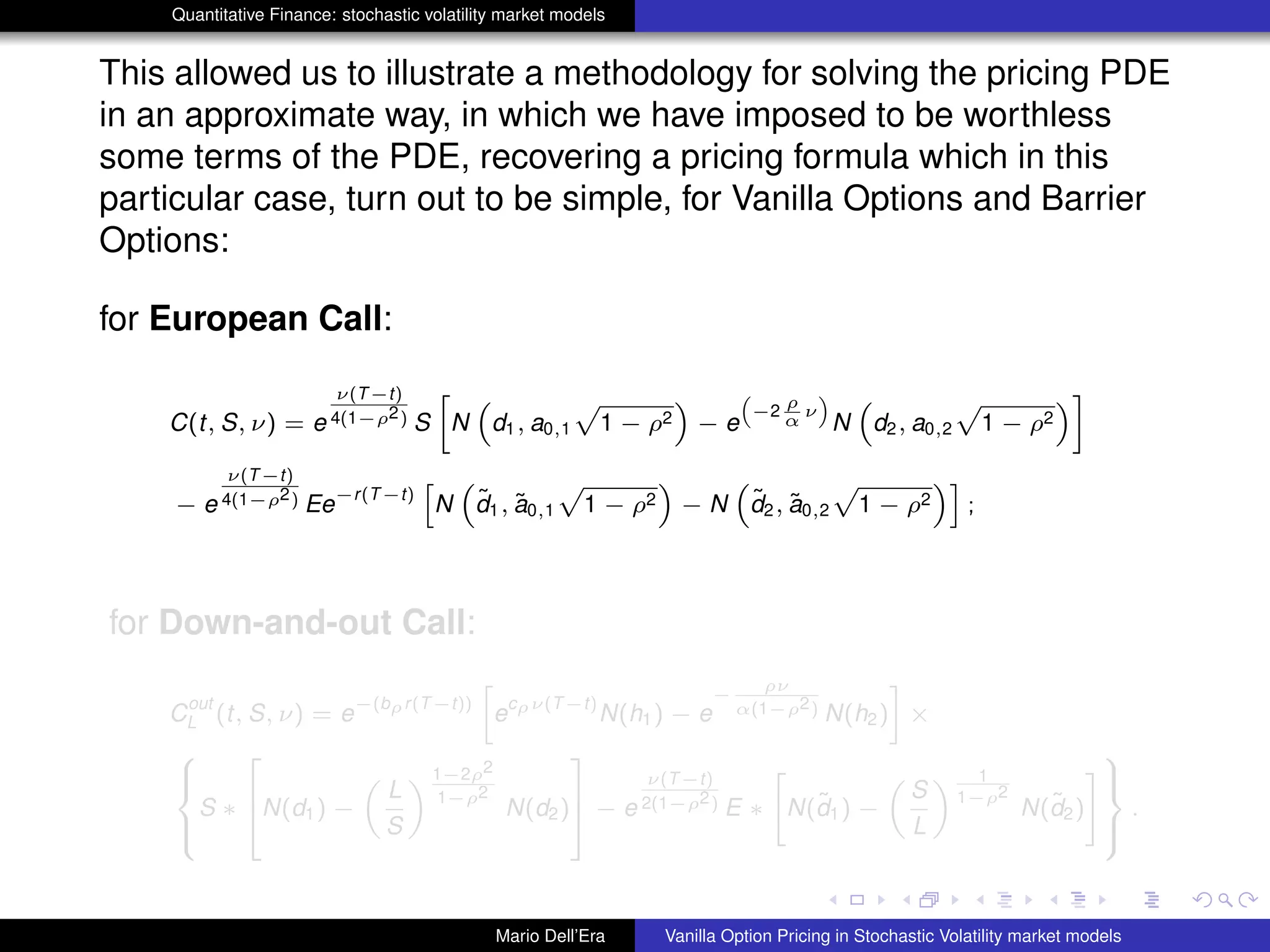
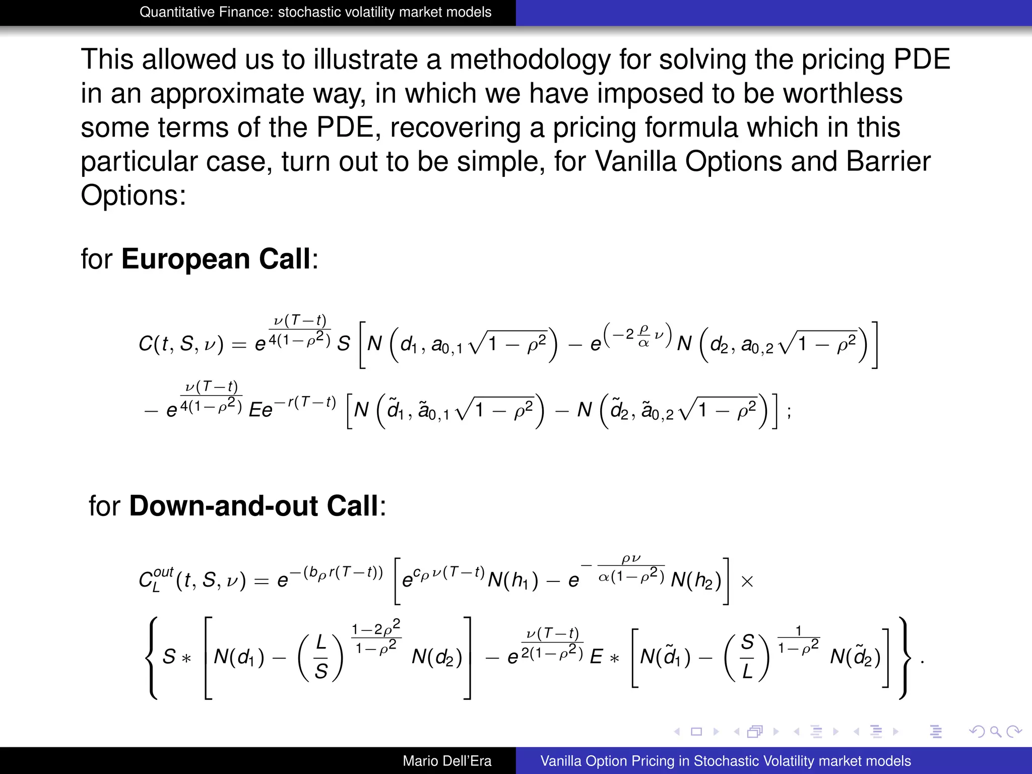
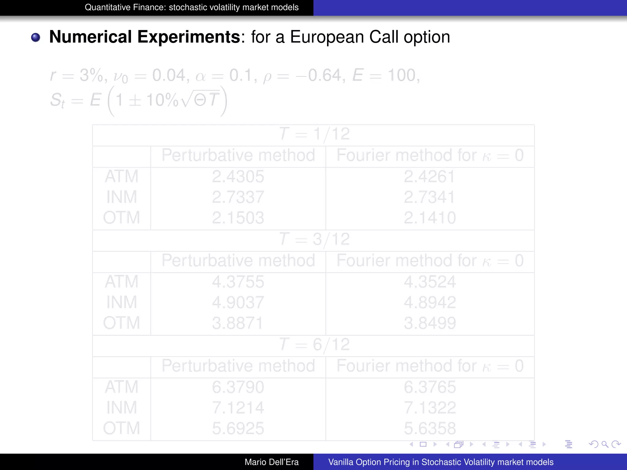
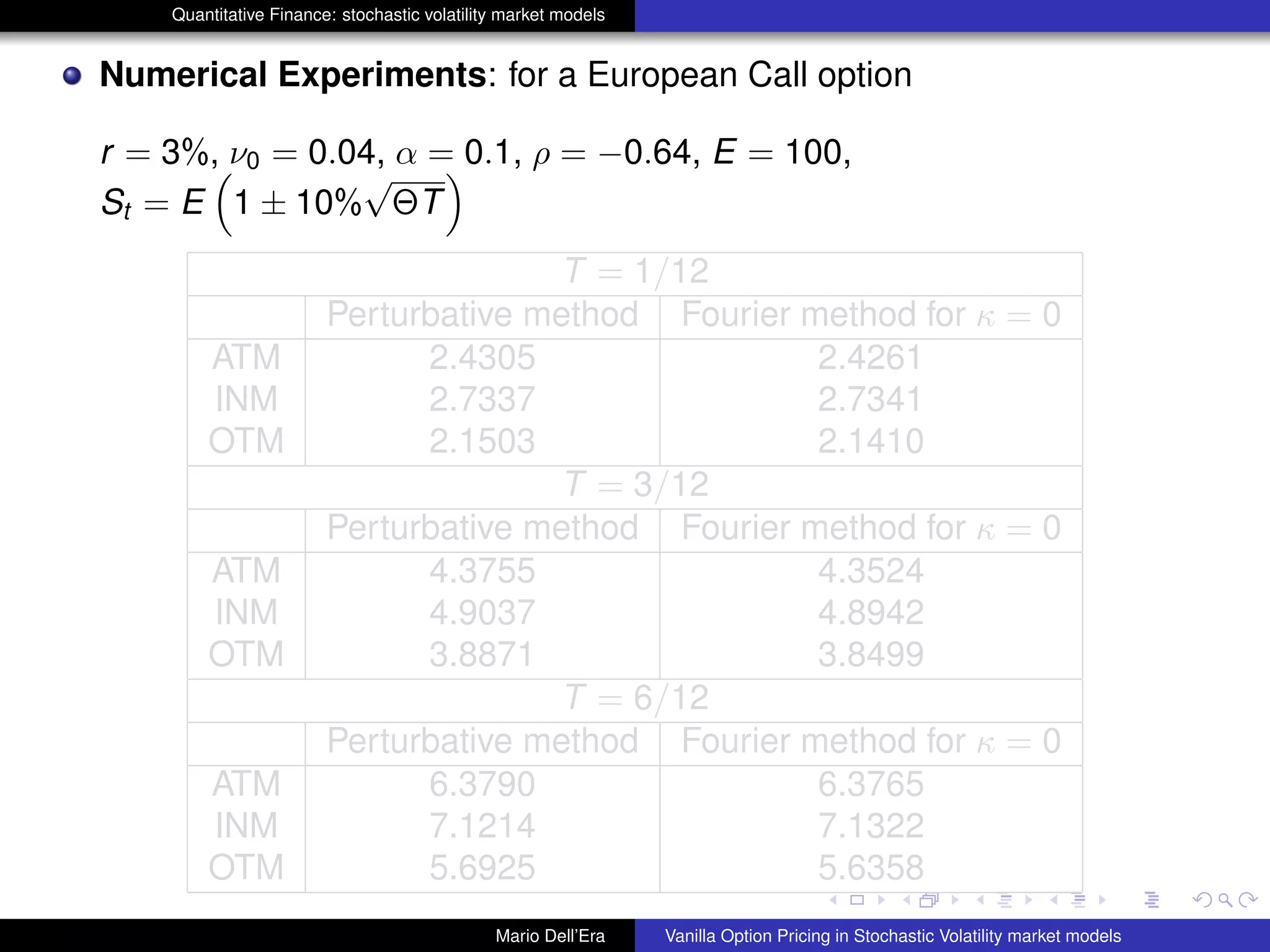
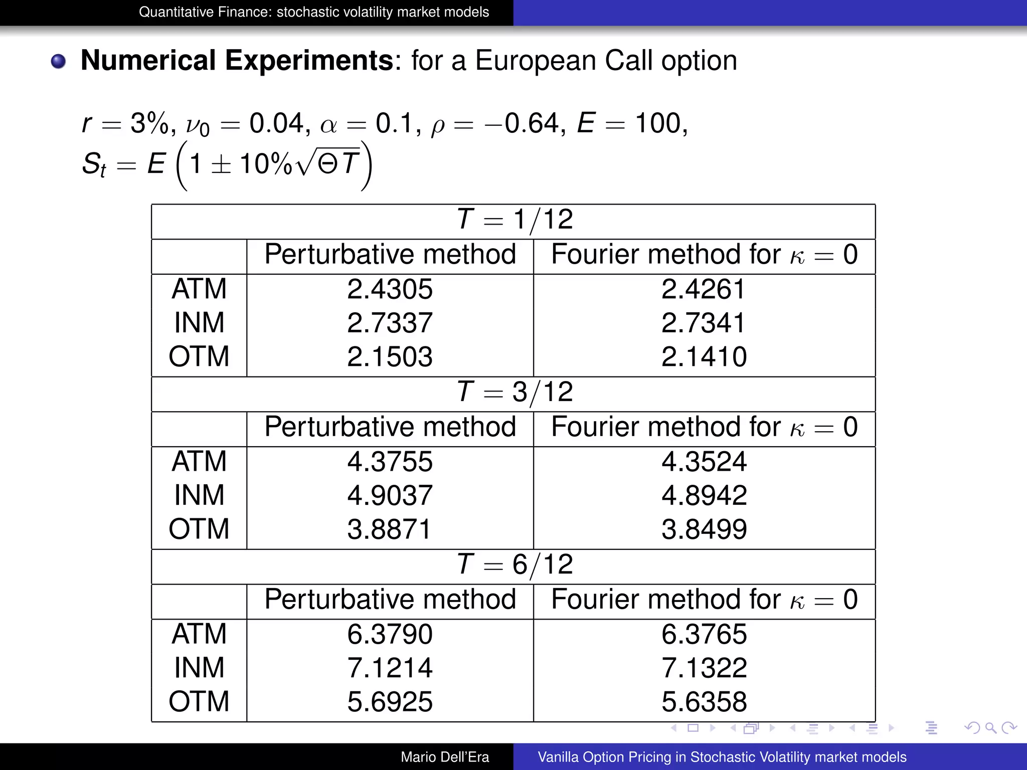
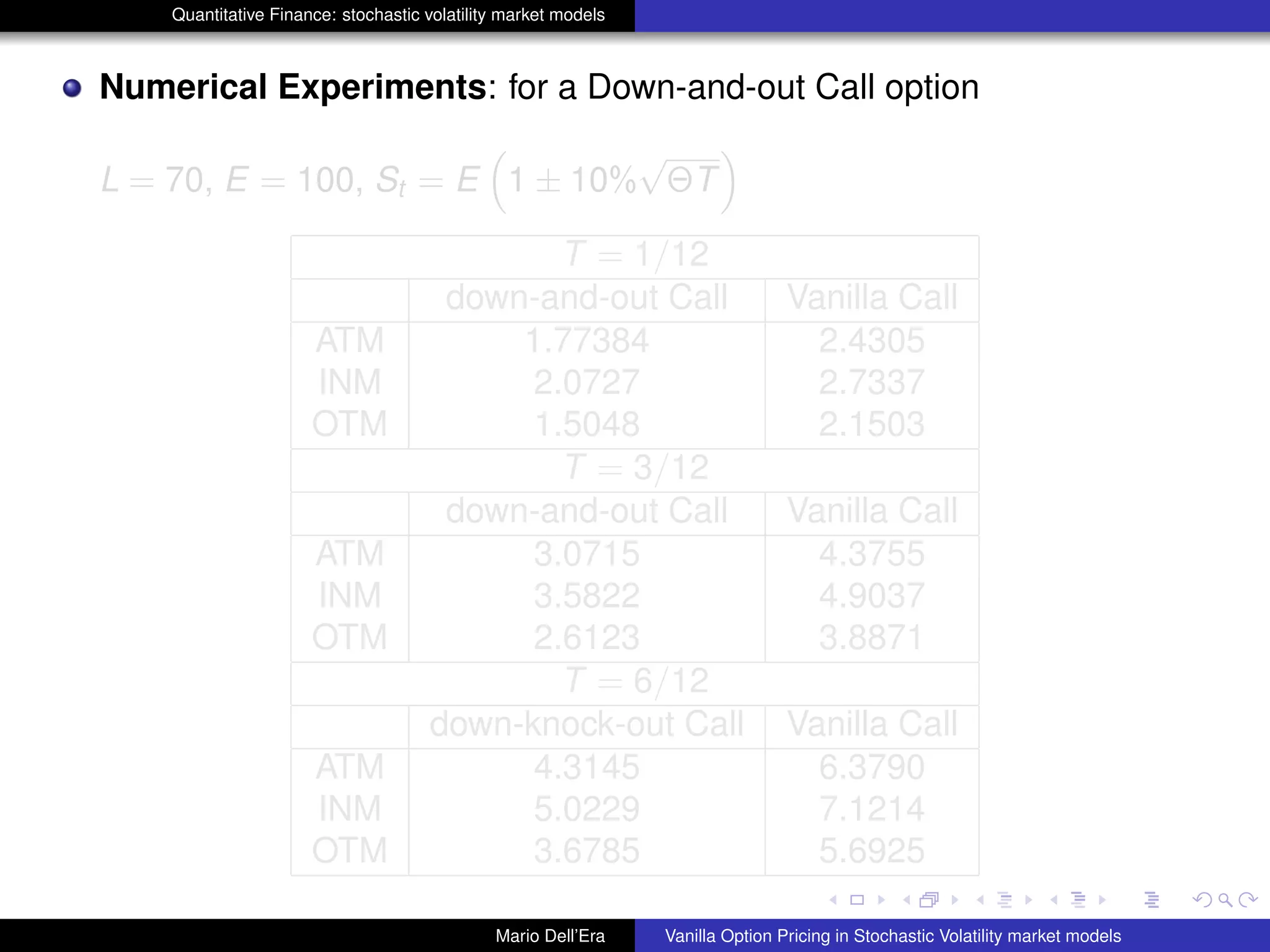
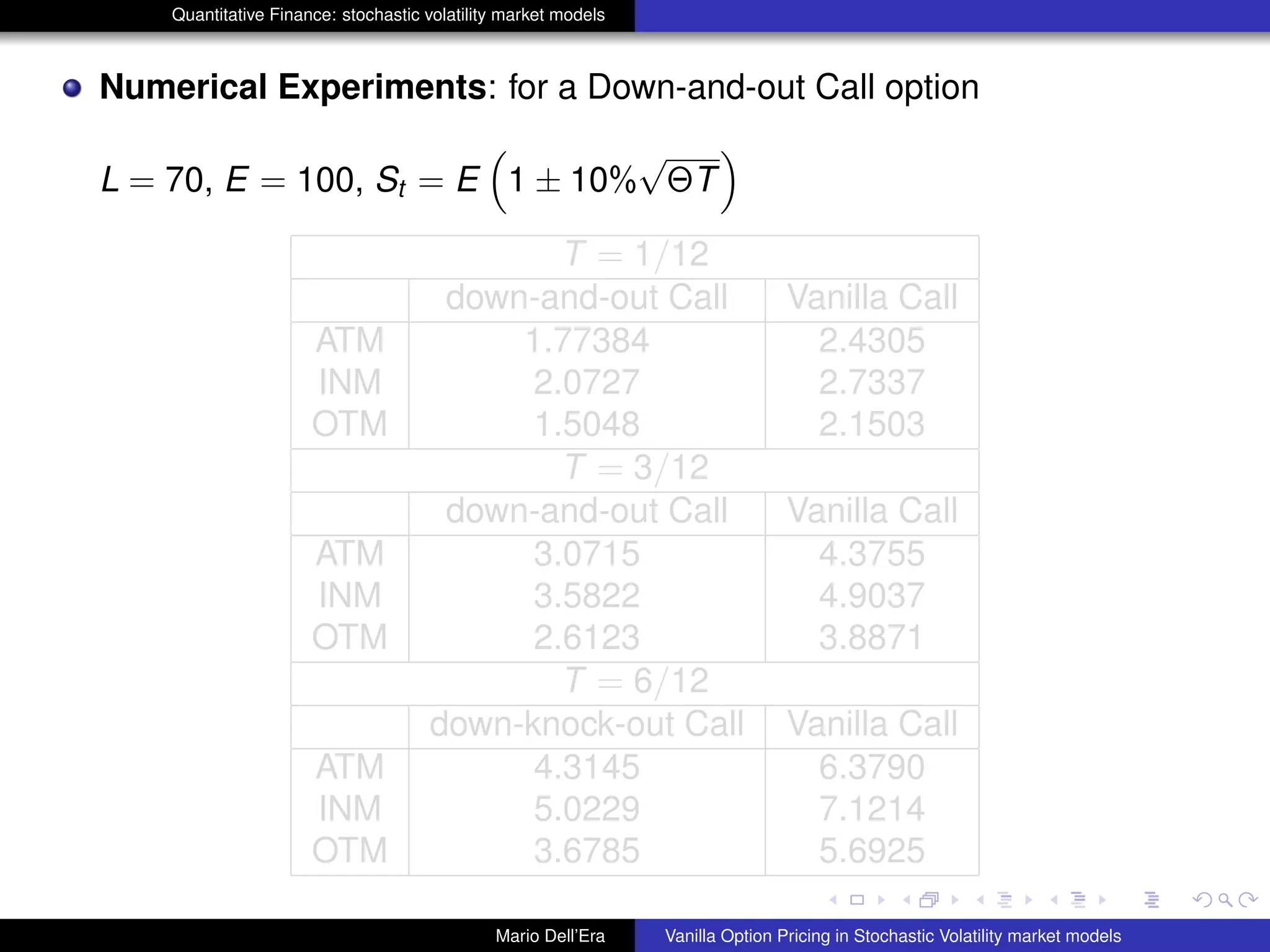
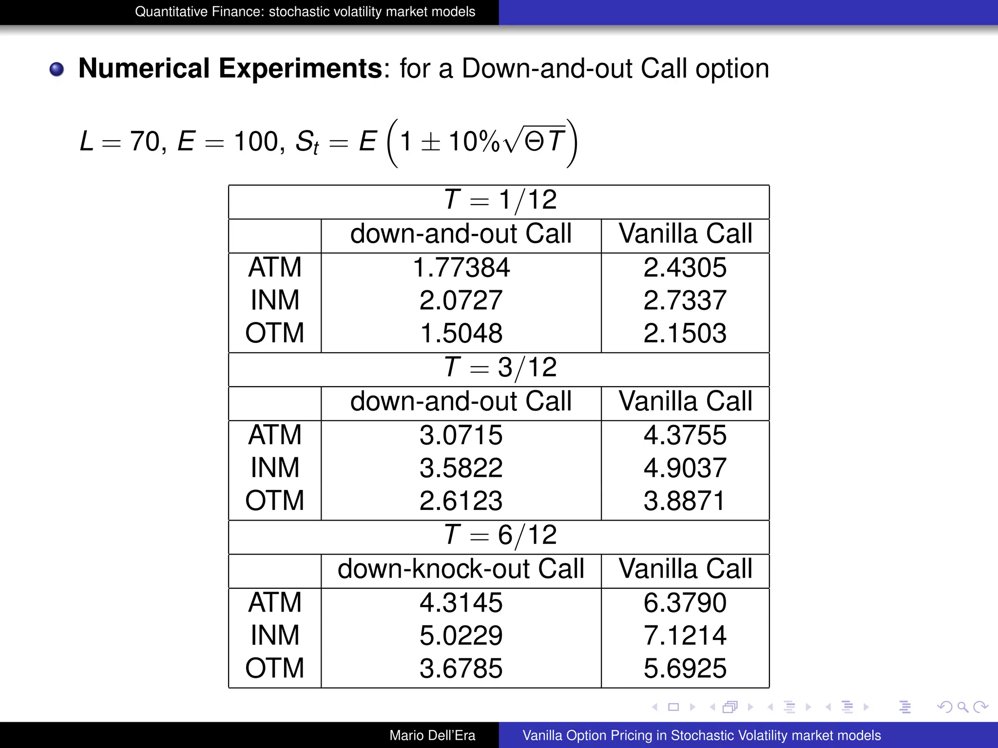
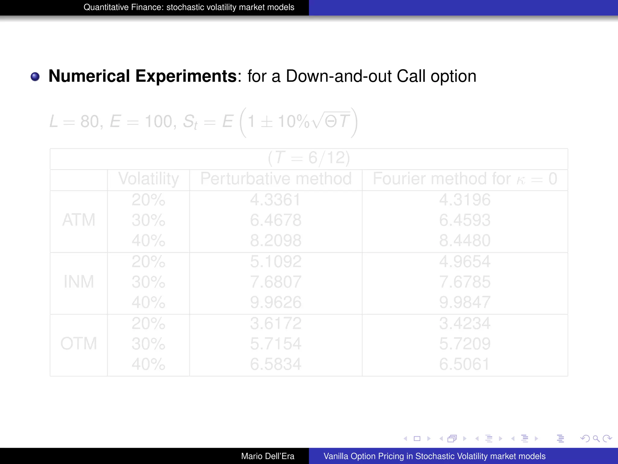
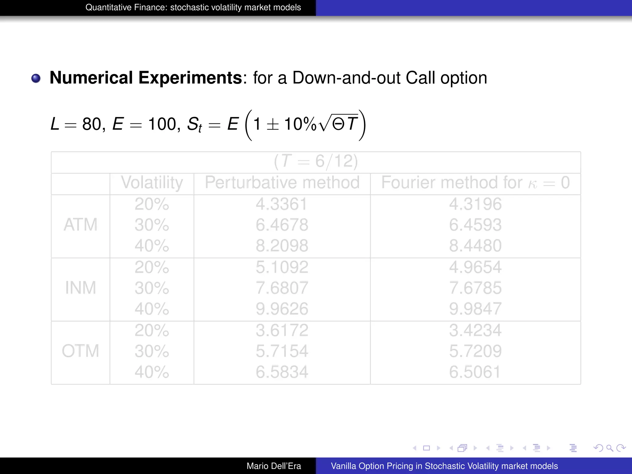
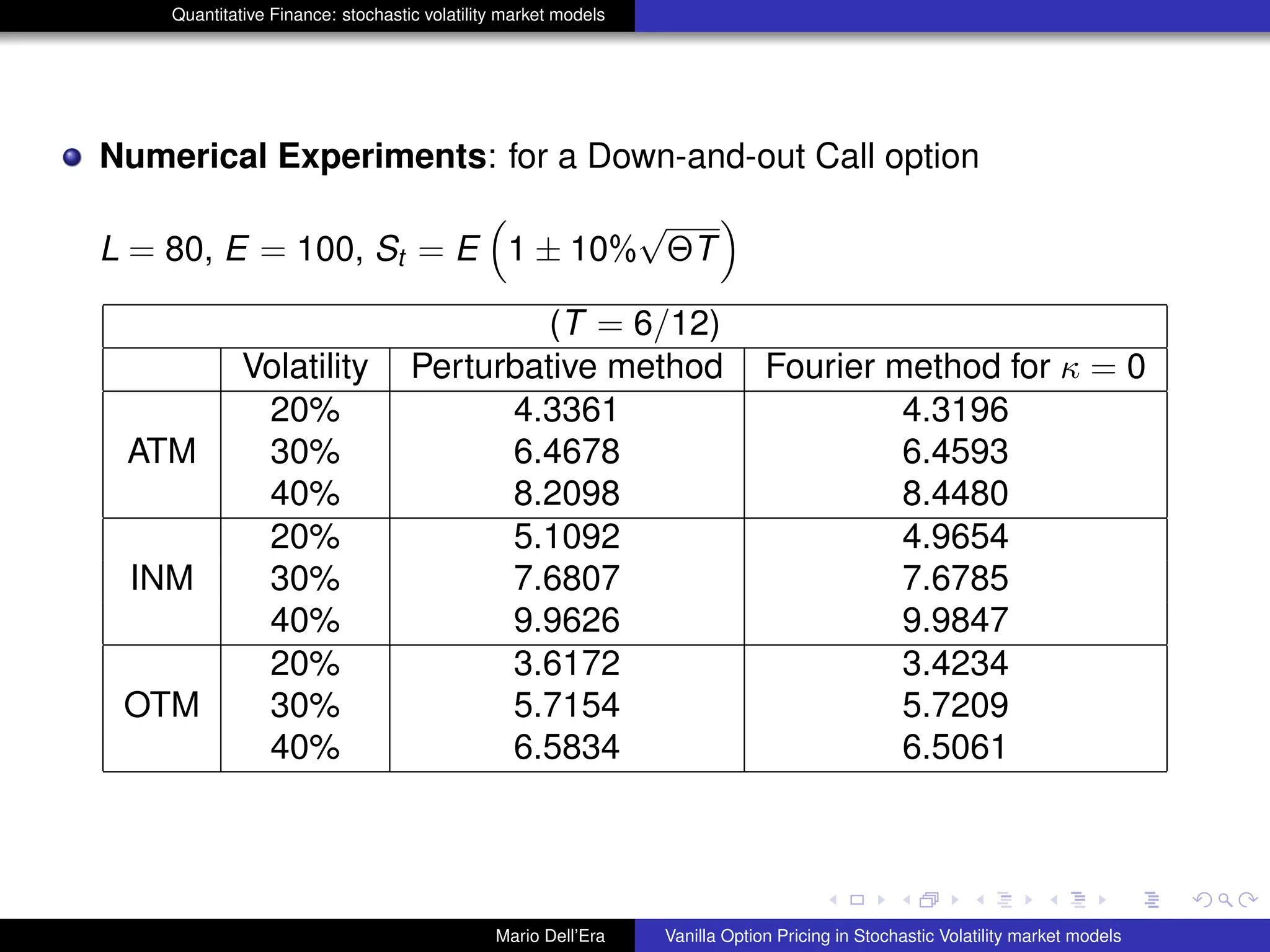
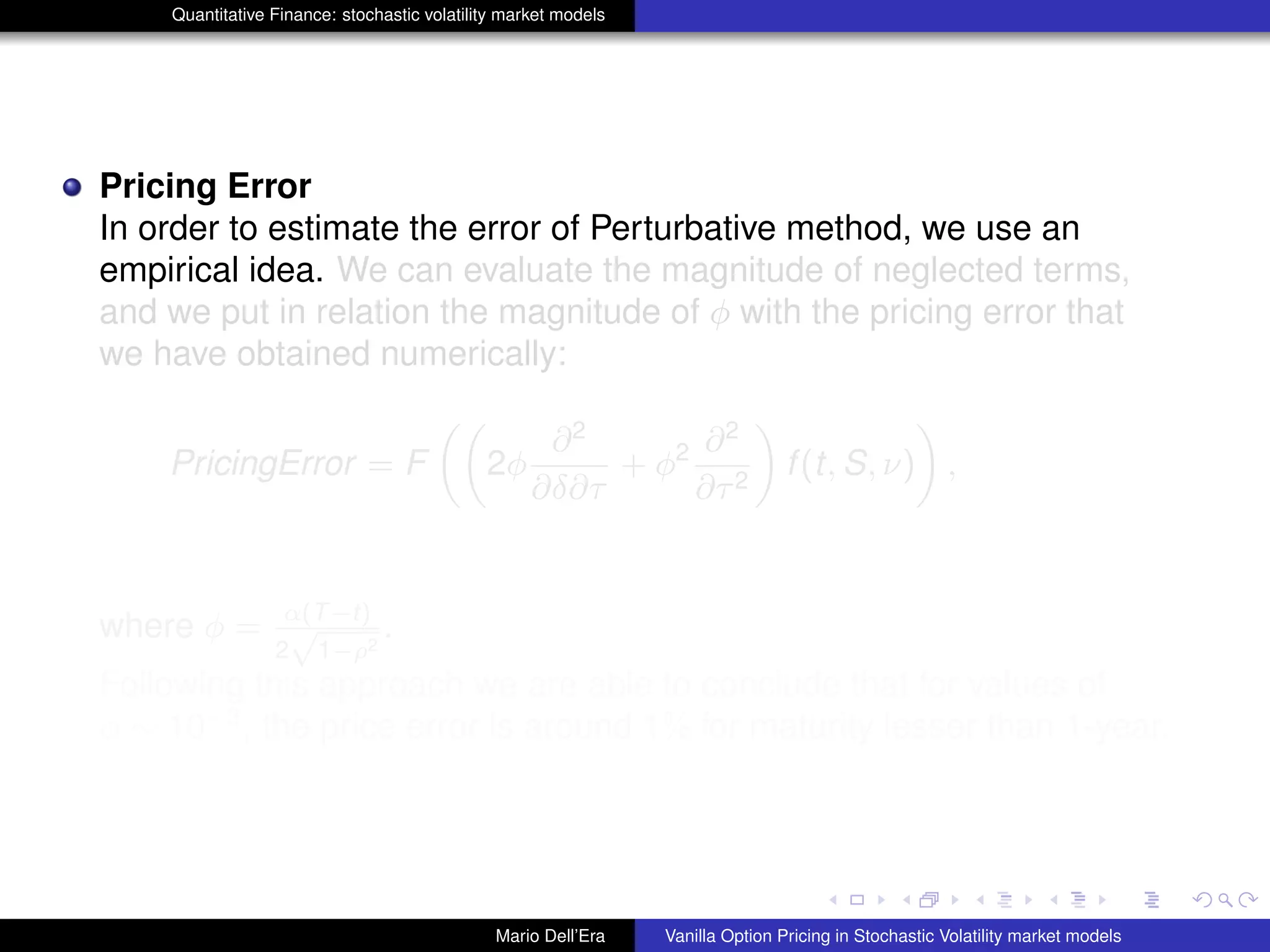
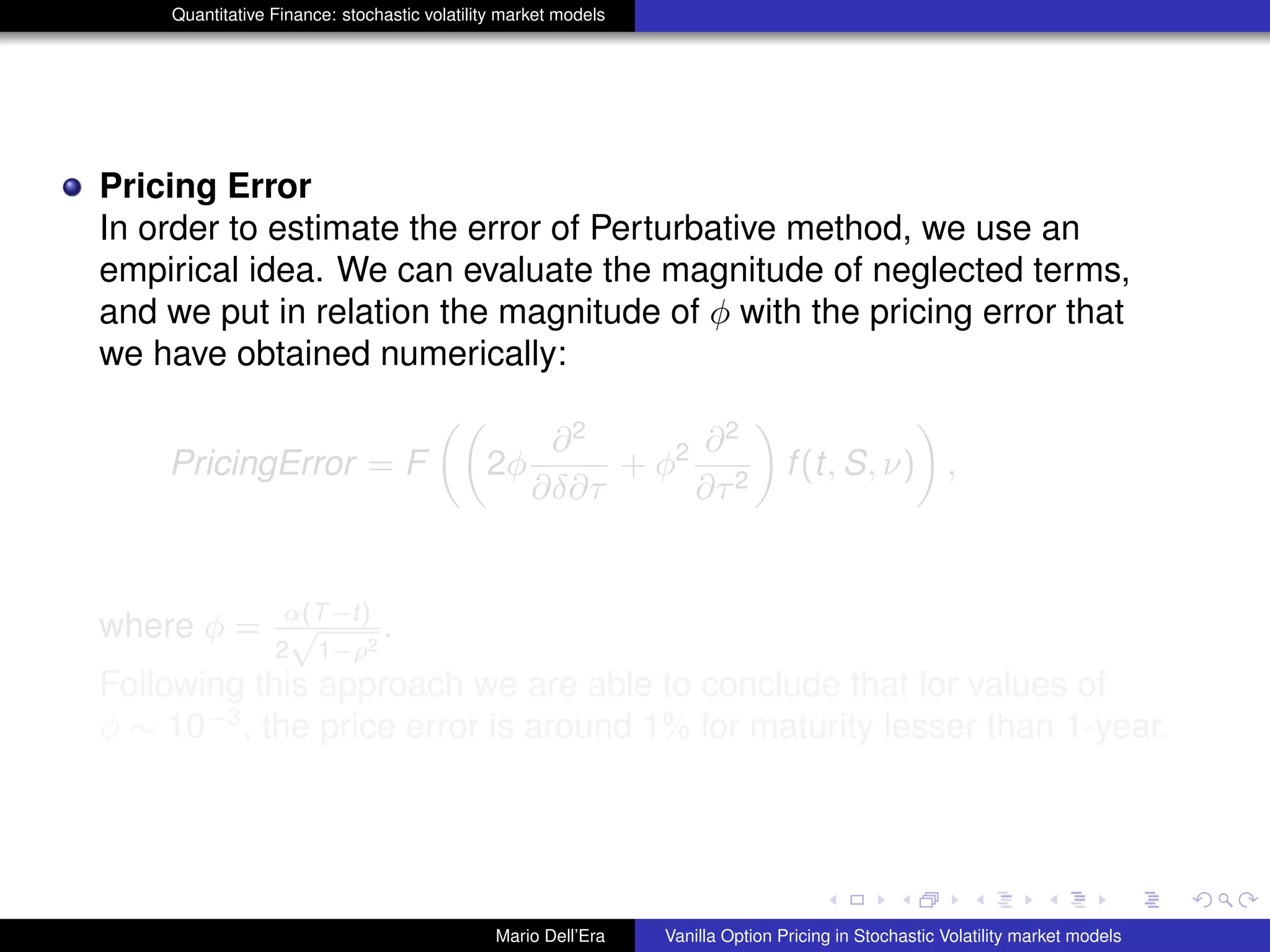
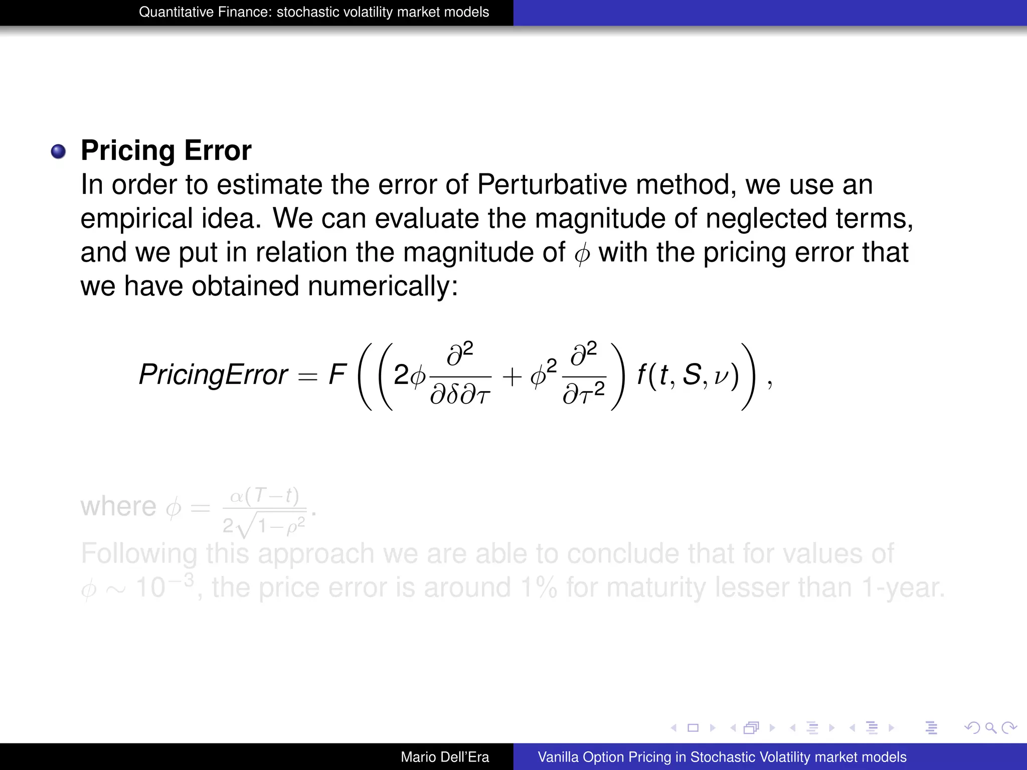
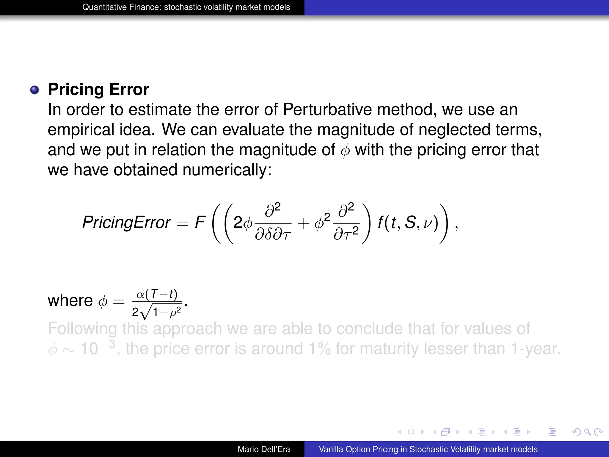
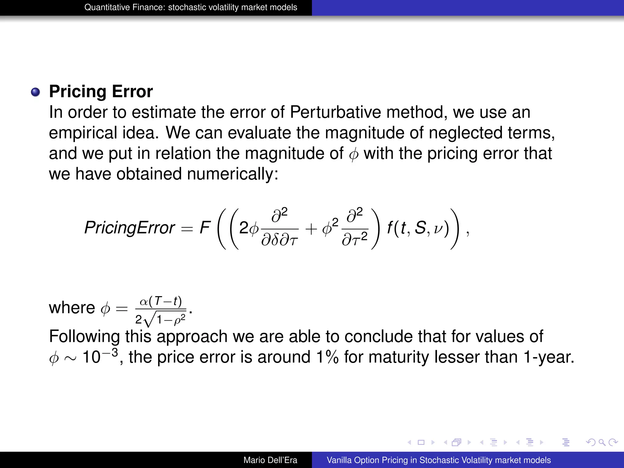
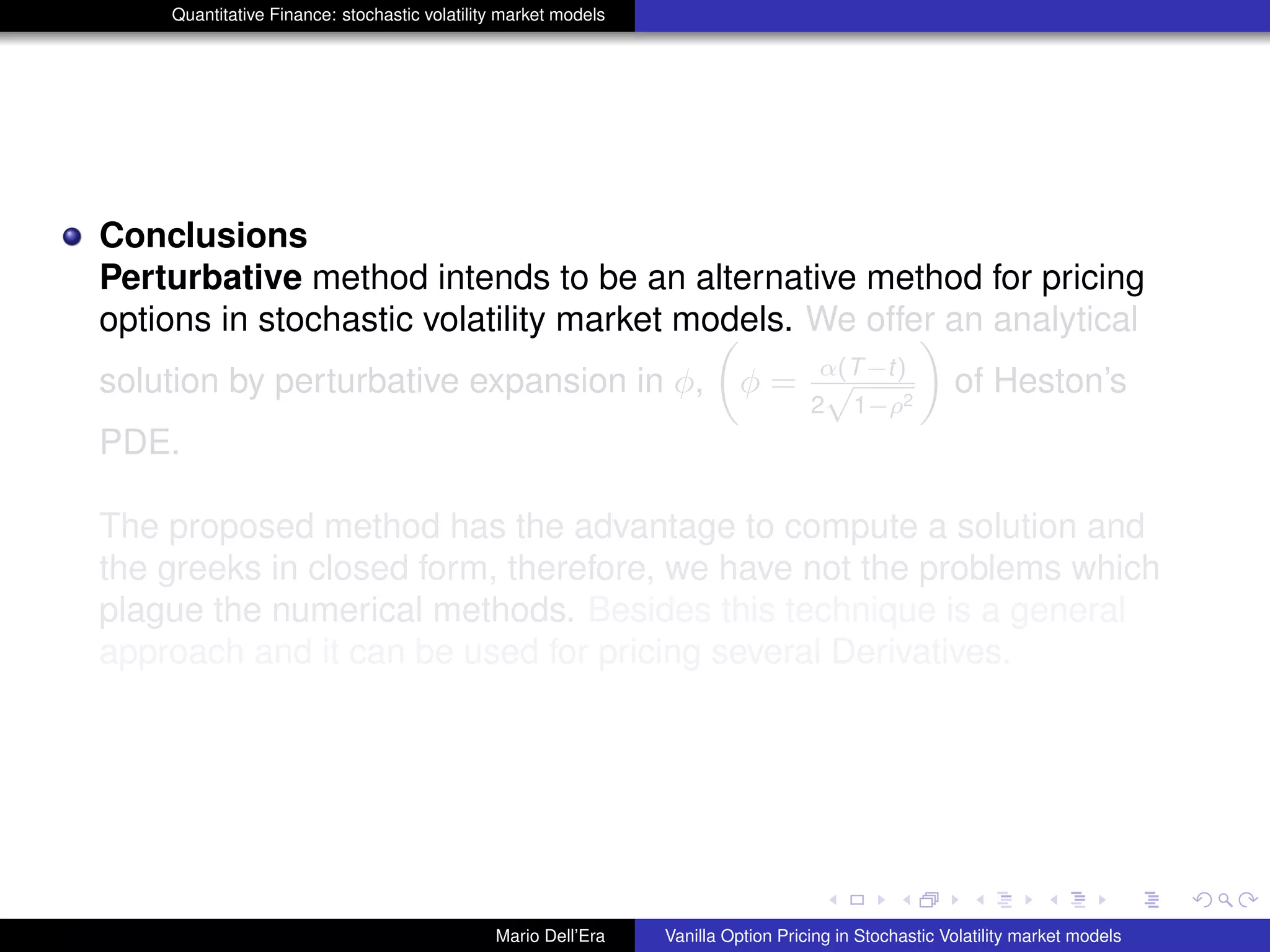
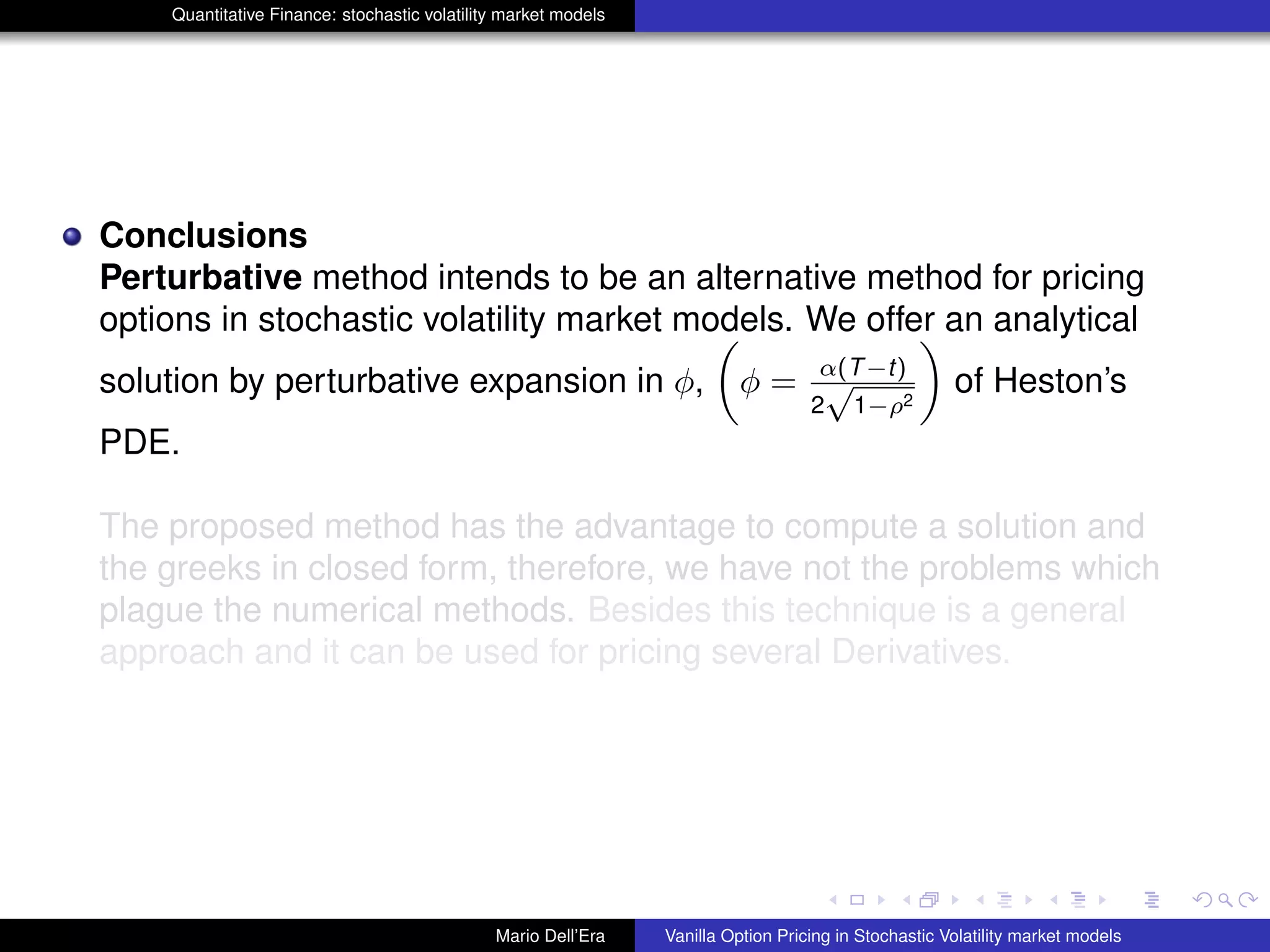
Quantitative Finance: stochastic volatility market models
Vanilla Option Pricing in Stochastic Volatility
market models
XIII WorkShop of Quantitative Finance
Mario Dell’Era
Scuola Superiore Sant’Anna
January 21, 2013
Mario Dell’Era Vanilla Option Pricing in Stochastic Volatility market models
Quantitative Finance: stochastic volatility market models
Stochastic Volatility Market Models
dSt = rSt dt + a(σt , St )d ˜W
(1)
t
dσt = b1(σt )dt + b2(σt )d ˜W
(2)
t
dBt = rBt dt
f(T, ST ) = φ(ST )
under a risk-neutral martingale measure Q.
Mario Dell’Era Vanilla Option Pricing in Stochastic Volatility market models
Quantitative Finance: stochastic volatility market models
Heston Model
dSt = rSt dt +
√
νt St d ˜W
(1)
t S ∈ [0, +∞)
dνt = K(Θ − νt )dt + α
√
νt d ˜W
(2)
t ν ∈ (0, +∞)
under a risk-neutral martingale measure Q.
From Itˆo’s lemma we have the following PDE:
∂f
∂t
+
1
2
νS2 ∂2
f
∂S2
+ρναS
∂2
f
∂S∂ν
+
1
2
να2 ∂2
f
∂ν2
+κ(Θ−ν)
∂f
∂ν
+rS
∂f
∂S
−rf = 0
Mario Dell’Era Vanilla Option Pricing in Stochastic Volatility market models
Quantitative Finance: stochastic volatility market models
Numerical methods
(1) Fourier Transform: S.L. Heston (1993)
(2) Finite Difference: T. Kluge (2002)
(3) Monte Carlo: B. Jourdain (2005)
Approximation method
(1) Analytic and Geometric Methods for Heat Kernel: I. Avramidi
(2007)
(2) Implied Volatility: M. Forde, A. Jacquier (2009)
(3) Geometrical Approximation method: M. Dell’Era (2010)
Mario Dell’Era Vanilla Option Pricing in Stochastic Volatility market models
Quantitative Finance: stochastic volatility market models
Perturbative Method: Heston model with zero drift
In this case we have discussed a particular choice of the volatility
price of risk in the Heston model, namely such that the drift term of
the risk-neutral stochastic volatility process is zero:
dSt = rSt dt +
√
νt St d ˜W
(1)
t ,
dνt = α
√
νt d ˜W
(2)
t , α ∈ R+
d ˜W
(1)
t d ˜W
(2)
t = ρdt, ρ ∈ (−1, +1)
dBt = rBt dt.
f(T, S, ν) = Φ(ST )
under a risk-neutral martingale measure Q.
Mario Dell’Era Vanilla Option Pricing in Stochastic Volatility market models
Quantitative Finance: stochastic volatility market models
From Itˇo’s lemma we have:
∂f
∂t
+
1
2
ν S2 ∂2
f
∂S2
+ 2ραS
∂2
f
∂S∂ν
+ α2 ∂2f
∂ν2
+ rS
∂f
∂S
− rf = 0
After three coordinate transformations we have:
∂f3
∂τ
− (1 − ρ2
)
∂2
f3
∂γ2
+
∂2
f3
∂δ2
+ 2φ
∂2
f3
∂δ∂τ
+ φ2 ∂2
f2
∂τ2
+ r
∂f3
∂γ
= 0
where φ = α(T−t)
2
√
1−ρ2
.
Since α ∼ 10−1
, for maturity date lesser than 1-year the term
(T − t) ∼ 10−1
and (2 1 − ρ2)−1
∼ 10−1
; thus φ ∼ 10−3
, φ2
∼ 10−6
.
Thus it is reasonable to approximate φ 0.
Mario Dell’Era Vanilla Option Pricing in Stochastic Volatility market models
Quantitative Finance: stochastic volatility market models
This allowed us to illustrate a methodology for solving the pricing PDE
in an approximate way, in which we have imposed to be worthless
some terms of the PDE, recovering a pricing formula which in this
particular case, turn out to be simple, for Vanilla Options and Barrier
Options:
for European Call:
C(t, S, ν) = e
ν(T−t)
4(1−ρ2) S
»
N
“
d1, a0,1
p
1 − ρ2
”
− e
“
−2
ρ
α
ν
”
N
“
d2, a0,2
p
1 − ρ2
”–
− e
ν(T−t)
4(1−ρ2) Ee
−r(T−t)
h
N
“
˜d1, ˜a0,1
p
1 − ρ2
”
− N
“
˜d2, ˜a0,2
p
1 − ρ2
”i
;
for Down-and-out Call:
C
out
L (t, S, ν) = e
−(bρr(T−t))
»
e
cρν(T−t)
N(h1) − e
−
ρν
α(1−ρ2) N(h2)
–
×
8
><
>:
S ∗
2
6
4N(d1) −
„
L
S
« 1−2ρ2
1−ρ2
N(d2)
3
7
5 − e
ν(T−t)
2(1−ρ2) E ∗
"
N(˜d1) −
„
S
L
« 1
1−ρ2
N(˜d2)
#
9
>=
>;
.
Mario Dell’Era Vanilla Option Pricing in Stochastic Volatility market models
Quantitative Finance: stochastic volatility market models
Numerical Experiments: for a European Call option
r = 3%, ν0 = 0.04, α = 0.1, ρ = −0.64, E = 100,
St = E 1 ± 10%
√
ΘT
T = 1/12
Perturbative method Fourier method for κ = 0
ATM 2.4305 2.4261
INM 2.7337 2.7341
OTM 2.1503 2.1410
T = 3/12
Perturbative method Fourier method for κ = 0
ATM 4.3755 4.3524
INM 4.9037 4.8942
OTM 3.8871 3.8499
T = 6/12
Perturbative method Fourier method for κ = 0
ATM 6.3790 6.3765
INM 7.1214 7.1322
OTM 5.6925 5.6358
Mario Dell’Era Vanilla Option Pricing in Stochastic Volatility market models
Quantitative Finance: stochastic volatility market models
Numerical Experiments: for a Down-and-out Call option
L = 70, E = 100, St = E 1 ± 10%
√
ΘT
T = 1/12
down-and-out Call Vanilla Call
ATM 1.77384 2.4305
INM 2.0727 2.7337
OTM 1.5048 2.1503
T = 3/12
down-and-out Call Vanilla Call
ATM 3.0715 4.3755
INM 3.5822 4.9037
OTM 2.6123 3.8871
T = 6/12
down-knock-out Call Vanilla Call
ATM 4.3145 6.3790
INM 5.0229 7.1214
OTM 3.6785 5.6925
Mario Dell’Era Vanilla Option Pricing in Stochastic Volatility market models
Quantitative Finance: stochastic volatility market models
Numerical Experiments: for a Down-and-out Call option
L = 80, E = 100, St = E 1 ± 10%
√
ΘT
(T = 6/12)
Volatility Perturbative method Fourier method for κ = 0
20% 4.3361 4.3196
ATM 30% 6.4678 6.4593
40% 8.2098 8.4480
20% 5.1092 4.9654
INM 30% 7.6807 7.6785
40% 9.9626 9.9847
20% 3.6172 3.4234
OTM 30% 5.7154 5.7209
40% 6.5834 6.5061
Mario Dell’Era Vanilla Option Pricing in Stochastic Volatility market models
Quantitative Finance: stochastic volatility market models
Pricing Error
In order to estimate the error of Perturbative method, we use an
empirical idea. We can evaluate the magnitude of neglected terms,
and we put in relation the magnitude of φ with the pricing error that
we have obtained numerically:
PricingError = F 2φ
∂2
∂δ∂τ
+ φ2 ∂2
∂τ2
f(t, S, ν) ,
where φ = α(T−t)
2
√
1−ρ2
.
Following this approach we are able to conclude that for values of
φ ∼ 10−3
, the price error is around 1% for maturity lesser than 1-year.
Mario Dell’Era Vanilla Option Pricing in Stochastic Volatility market models
Quantitative Finance: stochastic volatility market models
Conclusions
Perturbative method intends to be an alternative method for pricing
options in stochastic volatility market models. We offer an analytical
solution by perturbative expansion in φ, φ = α(T−t)
2
√
1−ρ2
of Heston’s
PDE.
The proposed method has the advantage to compute a solution and
the greeks in closed form, therefore, we have not the problems which
plague the numerical methods. Besides this technique is a general
approach and it can be used for pricing several Derivatives.
Mario Dell’Era Vanilla Option Pricing in Stochastic Volatility market models

Workshop 2012 of Quantitative Finance

  • 1.
    Quantitative Finance: stochasticvolatility market models Vanilla Option Pricing in Stochastic Volatility market models XIII WorkShop of Quantitative Finance Mario Dell’Era Scuola Superiore Sant’Anna January 21, 2013 Mario Dell’Era Vanilla Option Pricing in Stochastic Volatility market models
  • 2.
    Quantitative Finance: stochasticvolatility market models Stochastic Volatility Market Models dSt = rSt dt + a(σt , St )d ˜W (1) t dσt = b1(σt )dt + b2(σt )d ˜W (2) t dBt = rBt dt f(T, ST ) = φ(ST ) under a risk-neutral martingale measure Q. Mario Dell’Era Vanilla Option Pricing in Stochastic Volatility market models
  • 3.
    Quantitative Finance: stochasticvolatility market models Heston Model dSt = rSt dt + √ νt St d ˜W (1) t S ∈ [0, +∞) dνt = K(Θ − νt )dt + α √ νt d ˜W (2) t ν ∈ (0, +∞) under a risk-neutral martingale measure Q. From Itˆo’s lemma we have the following PDE: ∂f ∂t + 1 2 νS2 ∂2 f ∂S2 +ρναS ∂2 f ∂S∂ν + 1 2 να2 ∂2 f ∂ν2 +κ(Θ−ν) ∂f ∂ν +rS ∂f ∂S −rf = 0 Mario Dell’Era Vanilla Option Pricing in Stochastic Volatility market models
  • 4.
    Quantitative Finance: stochasticvolatility market models Heston Model dSt = rSt dt + √ νt St d ˜W (1) t S ∈ [0, +∞) dνt = K(Θ − νt )dt + α √ νt d ˜W (2) t ν ∈ (0, +∞) under a risk-neutral martingale measure Q. From Itˆo’s lemma we have the following PDE: ∂f ∂t + 1 2 νS2 ∂2 f ∂S2 +ρναS ∂2 f ∂S∂ν + 1 2 να2 ∂2 f ∂ν2 +κ(Θ−ν) ∂f ∂ν +rS ∂f ∂S −rf = 0 Mario Dell’Era Vanilla Option Pricing in Stochastic Volatility market models
  • 5.
    Quantitative Finance: stochasticvolatility market models Numerical methods (1) Fourier Transform: S.L. Heston (1993) (2) Finite Difference: T. Kluge (2002) (3) Monte Carlo: B. Jourdain (2005) Approximation method (1) Analytic and Geometric Methods for Heat Kernel: I. Avramidi (2007) (2) Implied Volatility: M. Forde, A. Jacquier (2009) (3) Geometrical Approximation method: M. Dell’Era (2010) Mario Dell’Era Vanilla Option Pricing in Stochastic Volatility market models
  • 6.
    Quantitative Finance: stochasticvolatility market models Numerical methods (1) Fourier Transform: S.L. Heston (1993) (2) Finite Difference: T. Kluge (2002) (3) Monte Carlo: B. Jourdain (2005) Approximation method (1) Analytic and Geometric Methods for Heat Kernel: I. Avramidi (2007) (2) Implied Volatility: M. Forde, A. Jacquier (2009) (3) Geometrical Approximation method: M. Dell’Era (2010) Mario Dell’Era Vanilla Option Pricing in Stochastic Volatility market models
  • 7.
    Quantitative Finance: stochasticvolatility market models Numerical methods (1) Fourier Transform: S.L. Heston (1993) (2) Finite Difference: T. Kluge (2002) (3) Monte Carlo: B. Jourdain (2005) Approximation method (1) Analytic and Geometric Methods for Heat Kernel: I. Avramidi (2007) (2) Implied Volatility: M. Forde, A. Jacquier (2009) (3) Geometrical Approximation method: M. Dell’Era (2010) Mario Dell’Era Vanilla Option Pricing in Stochastic Volatility market models
  • 8.
    Quantitative Finance: stochasticvolatility market models Numerical methods (1) Fourier Transform: S.L. Heston (1993) (2) Finite Difference: T. Kluge (2002) (3) Monte Carlo: B. Jourdain (2005) Approximation method (1) Analytic and Geometric Methods for Heat Kernel: I. Avramidi (2007) (2) Implied Volatility: M. Forde, A. Jacquier (2009) (3) Geometrical Approximation method: M. Dell’Era (2010) Mario Dell’Era Vanilla Option Pricing in Stochastic Volatility market models
  • 9.
    Quantitative Finance: stochasticvolatility market models Numerical methods (1) Fourier Transform: S.L. Heston (1993) (2) Finite Difference: T. Kluge (2002) (3) Monte Carlo: B. Jourdain (2005) Approximation method (1) Analytic and Geometric Methods for Heat Kernel: I. Avramidi (2007) (2) Implied Volatility: M. Forde, A. Jacquier (2009) (3) Geometrical Approximation method: M. Dell’Era (2010) Mario Dell’Era Vanilla Option Pricing in Stochastic Volatility market models
  • 10.
    Quantitative Finance: stochasticvolatility market models Numerical methods (1) Fourier Transform: S.L. Heston (1993) (2) Finite Difference: T. Kluge (2002) (3) Monte Carlo: B. Jourdain (2005) Approximation method (1) Analytic and Geometric Methods for Heat Kernel: I. Avramidi (2007) (2) Implied Volatility: M. Forde, A. Jacquier (2009) (3) Geometrical Approximation method: M. Dell’Era (2010) Mario Dell’Era Vanilla Option Pricing in Stochastic Volatility market models
  • 11.
    Quantitative Finance: stochasticvolatility market models Numerical methods (1) Fourier Transform: S.L. Heston (1993) (2) Finite Difference: T. Kluge (2002) (3) Monte Carlo: B. Jourdain (2005) Approximation method (1) Analytic and Geometric Methods for Heat Kernel: I. Avramidi (2007) (2) Implied Volatility: M. Forde, A. Jacquier (2009) (3) Geometrical Approximation method: M. Dell’Era (2010) Mario Dell’Era Vanilla Option Pricing in Stochastic Volatility market models
  • 12.
    Quantitative Finance: stochasticvolatility market models Numerical methods (1) Fourier Transform: S.L. Heston (1993) (2) Finite Difference: T. Kluge (2002) (3) Monte Carlo: B. Jourdain (2005) Approximation method (1) Analytic and Geometric Methods for Heat Kernel: I. Avramidi (2007) (2) Implied Volatility: M. Forde, A. Jacquier (2009) (3) Geometrical Approximation method: M. Dell’Era (2010) Mario Dell’Era Vanilla Option Pricing in Stochastic Volatility market models
  • 13.
    Quantitative Finance: stochasticvolatility market models Perturbative Method: Heston model with zero drift In this case we have discussed a particular choice of the volatility price of risk in the Heston model, namely such that the drift term of the risk-neutral stochastic volatility process is zero: dSt = rSt dt + √ νt St d ˜W (1) t , dνt = α √ νt d ˜W (2) t , α ∈ R+ d ˜W (1) t d ˜W (2) t = ρdt, ρ ∈ (−1, +1) dBt = rBt dt. f(T, S, ν) = Φ(ST ) under a risk-neutral martingale measure Q. Mario Dell’Era Vanilla Option Pricing in Stochastic Volatility market models
  • 14.
    Quantitative Finance: stochasticvolatility market models Perturbative Method: Heston model with zero drift In this case we have discussed a particular choice of the volatility price of risk in the Heston model, namely such that the drift term of the risk-neutral stochastic volatility process is zero: dSt = rSt dt + √ νt St d ˜W (1) t , dνt = α √ νt d ˜W (2) t , α ∈ R+ d ˜W (1) t d ˜W (2) t = ρdt, ρ ∈ (−1, +1) dBt = rBt dt. f(T, S, ν) = Φ(ST ) under a risk-neutral martingale measure Q. Mario Dell’Era Vanilla Option Pricing in Stochastic Volatility market models
  • 15.
    Quantitative Finance: stochasticvolatility market models From Itˇo’s lemma we have: ∂f ∂t + 1 2 ν S2 ∂2 f ∂S2 + 2ραS ∂2 f ∂S∂ν + α2 ∂2f ∂ν2 + rS ∂f ∂S − rf = 0 After three coordinate transformations we have: ∂f3 ∂τ − (1 − ρ2 ) ∂2 f3 ∂γ2 + ∂2 f3 ∂δ2 + 2φ ∂2 f3 ∂δ∂τ + φ2 ∂2 f2 ∂τ2 + r ∂f3 ∂γ = 0 where φ = α(T−t) 2 √ 1−ρ2 . Since α ∼ 10−1 , for maturity date lesser than 1-year the term (T − t) ∼ 10−1 and (2 1 − ρ2)−1 ∼ 10−1 ; thus φ ∼ 10−3 , φ2 ∼ 10−6 . Thus it is reasonable to approximate φ 0. Mario Dell’Era Vanilla Option Pricing in Stochastic Volatility market models
  • 16.
    Quantitative Finance: stochasticvolatility market models From Itˇo’s lemma we have: ∂f ∂t + 1 2 ν S2 ∂2 f ∂S2 + 2ραS ∂2 f ∂S∂ν + α2 ∂2f ∂ν2 + rS ∂f ∂S − rf = 0 After three coordinate transformations we have: ∂f3 ∂τ − (1 − ρ2 ) ∂2 f3 ∂γ2 + ∂2 f3 ∂δ2 + 2φ ∂2 f3 ∂δ∂τ + φ2 ∂2 f2 ∂τ2 + r ∂f3 ∂γ = 0 where φ = α(T−t) 2 √ 1−ρ2 . Since α ∼ 10−1 , for maturity date lesser than 1-year the term (T − t) ∼ 10−1 and (2 1 − ρ2)−1 ∼ 10−1 ; thus φ ∼ 10−3 , φ2 ∼ 10−6 . Thus it is reasonable to approximate φ 0. Mario Dell’Era Vanilla Option Pricing in Stochastic Volatility market models
  • 17.
    Quantitative Finance: stochasticvolatility market models From Itˇo’s lemma we have: ∂f ∂t + 1 2 ν S2 ∂2 f ∂S2 + 2ραS ∂2 f ∂S∂ν + α2 ∂2f ∂ν2 + rS ∂f ∂S − rf = 0 After three coordinate transformations we have: ∂f3 ∂τ − (1 − ρ2 ) ∂2 f3 ∂γ2 + ∂2 f3 ∂δ2 + 2φ ∂2 f3 ∂δ∂τ + φ2 ∂2 f2 ∂τ2 + r ∂f3 ∂γ = 0 where φ = α(T−t) 2 √ 1−ρ2 . Since α ∼ 10−1 , for maturity date lesser than 1-year the term (T − t) ∼ 10−1 and (2 1 − ρ2)−1 ∼ 10−1 ; thus φ ∼ 10−3 , φ2 ∼ 10−6 . Thus it is reasonable to approximate φ 0. Mario Dell’Era Vanilla Option Pricing in Stochastic Volatility market models
  • 18.
    Quantitative Finance: stochasticvolatility market models This allowed us to illustrate a methodology for solving the pricing PDE in an approximate way, in which we have imposed to be worthless some terms of the PDE, recovering a pricing formula which in this particular case, turn out to be simple, for Vanilla Options and Barrier Options: for European Call: C(t, S, ν) = e ν(T−t) 4(1−ρ2) S » N “ d1, a0,1 p 1 − ρ2 ” − e “ −2 ρ α ν ” N “ d2, a0,2 p 1 − ρ2 ”– − e ν(T−t) 4(1−ρ2) Ee −r(T−t) h N “ ˜d1, ˜a0,1 p 1 − ρ2 ” − N “ ˜d2, ˜a0,2 p 1 − ρ2 ”i ; for Down-and-out Call: C out L (t, S, ν) = e −(bρr(T−t)) » e cρν(T−t) N(h1) − e − ρν α(1−ρ2) N(h2) – × 8 >< >: S ∗ 2 6 4N(d1) − „ L S « 1−2ρ2 1−ρ2 N(d2) 3 7 5 − e ν(T−t) 2(1−ρ2) E ∗ " N(˜d1) − „ S L « 1 1−ρ2 N(˜d2) # 9 >= >; . Mario Dell’Era Vanilla Option Pricing in Stochastic Volatility market models
  • 19.
    Quantitative Finance: stochasticvolatility market models This allowed us to illustrate a methodology for solving the pricing PDE in an approximate way, in which we have imposed to be worthless some terms of the PDE, recovering a pricing formula which in this particular case, turn out to be simple, for Vanilla Options and Barrier Options: for European Call: C(t, S, ν) = e ν(T−t) 4(1−ρ2) S » N “ d1, a0,1 p 1 − ρ2 ” − e “ −2 ρ α ν ” N “ d2, a0,2 p 1 − ρ2 ”– − e ν(T−t) 4(1−ρ2) Ee −r(T−t) h N “ ˜d1, ˜a0,1 p 1 − ρ2 ” − N “ ˜d2, ˜a0,2 p 1 − ρ2 ”i ; for Down-and-out Call: C out L (t, S, ν) = e −(bρr(T−t)) » e cρν(T−t) N(h1) − e − ρν α(1−ρ2) N(h2) – × 8 >< >: S ∗ 2 6 4N(d1) − „ L S « 1−2ρ2 1−ρ2 N(d2) 3 7 5 − e ν(T−t) 2(1−ρ2) E ∗ " N(˜d1) − „ S L « 1 1−ρ2 N(˜d2) # 9 >= >; . Mario Dell’Era Vanilla Option Pricing in Stochastic Volatility market models
  • 20.
    Quantitative Finance: stochasticvolatility market models This allowed us to illustrate a methodology for solving the pricing PDE in an approximate way, in which we have imposed to be worthless some terms of the PDE, recovering a pricing formula which in this particular case, turn out to be simple, for Vanilla Options and Barrier Options: for European Call: C(t, S, ν) = e ν(T−t) 4(1−ρ2) S » N “ d1, a0,1 p 1 − ρ2 ” − e “ −2 ρ α ν ” N “ d2, a0,2 p 1 − ρ2 ”– − e ν(T−t) 4(1−ρ2) Ee −r(T−t) h N “ ˜d1, ˜a0,1 p 1 − ρ2 ” − N “ ˜d2, ˜a0,2 p 1 − ρ2 ”i ; for Down-and-out Call: C out L (t, S, ν) = e −(bρr(T−t)) » e cρν(T−t) N(h1) − e − ρν α(1−ρ2) N(h2) – × 8 >< >: S ∗ 2 6 4N(d1) − „ L S « 1−2ρ2 1−ρ2 N(d2) 3 7 5 − e ν(T−t) 2(1−ρ2) E ∗ " N(˜d1) − „ S L « 1 1−ρ2 N(˜d2) # 9 >= >; . Mario Dell’Era Vanilla Option Pricing in Stochastic Volatility market models
  • 21.
    Quantitative Finance: stochasticvolatility market models Numerical Experiments: for a European Call option r = 3%, ν0 = 0.04, α = 0.1, ρ = −0.64, E = 100, St = E 1 ± 10% √ ΘT T = 1/12 Perturbative method Fourier method for κ = 0 ATM 2.4305 2.4261 INM 2.7337 2.7341 OTM 2.1503 2.1410 T = 3/12 Perturbative method Fourier method for κ = 0 ATM 4.3755 4.3524 INM 4.9037 4.8942 OTM 3.8871 3.8499 T = 6/12 Perturbative method Fourier method for κ = 0 ATM 6.3790 6.3765 INM 7.1214 7.1322 OTM 5.6925 5.6358 Mario Dell’Era Vanilla Option Pricing in Stochastic Volatility market models
  • 22.
    Quantitative Finance: stochasticvolatility market models Numerical Experiments: for a European Call option r = 3%, ν0 = 0.04, α = 0.1, ρ = −0.64, E = 100, St = E 1 ± 10% √ ΘT T = 1/12 Perturbative method Fourier method for κ = 0 ATM 2.4305 2.4261 INM 2.7337 2.7341 OTM 2.1503 2.1410 T = 3/12 Perturbative method Fourier method for κ = 0 ATM 4.3755 4.3524 INM 4.9037 4.8942 OTM 3.8871 3.8499 T = 6/12 Perturbative method Fourier method for κ = 0 ATM 6.3790 6.3765 INM 7.1214 7.1322 OTM 5.6925 5.6358 Mario Dell’Era Vanilla Option Pricing in Stochastic Volatility market models
  • 23.
    Quantitative Finance: stochasticvolatility market models Numerical Experiments: for a European Call option r = 3%, ν0 = 0.04, α = 0.1, ρ = −0.64, E = 100, St = E 1 ± 10% √ ΘT T = 1/12 Perturbative method Fourier method for κ = 0 ATM 2.4305 2.4261 INM 2.7337 2.7341 OTM 2.1503 2.1410 T = 3/12 Perturbative method Fourier method for κ = 0 ATM 4.3755 4.3524 INM 4.9037 4.8942 OTM 3.8871 3.8499 T = 6/12 Perturbative method Fourier method for κ = 0 ATM 6.3790 6.3765 INM 7.1214 7.1322 OTM 5.6925 5.6358 Mario Dell’Era Vanilla Option Pricing in Stochastic Volatility market models
  • 24.
    Quantitative Finance: stochasticvolatility market models Numerical Experiments: for a Down-and-out Call option L = 70, E = 100, St = E 1 ± 10% √ ΘT T = 1/12 down-and-out Call Vanilla Call ATM 1.77384 2.4305 INM 2.0727 2.7337 OTM 1.5048 2.1503 T = 3/12 down-and-out Call Vanilla Call ATM 3.0715 4.3755 INM 3.5822 4.9037 OTM 2.6123 3.8871 T = 6/12 down-knock-out Call Vanilla Call ATM 4.3145 6.3790 INM 5.0229 7.1214 OTM 3.6785 5.6925 Mario Dell’Era Vanilla Option Pricing in Stochastic Volatility market models
  • 25.
    Quantitative Finance: stochasticvolatility market models Numerical Experiments: for a Down-and-out Call option L = 70, E = 100, St = E 1 ± 10% √ ΘT T = 1/12 down-and-out Call Vanilla Call ATM 1.77384 2.4305 INM 2.0727 2.7337 OTM 1.5048 2.1503 T = 3/12 down-and-out Call Vanilla Call ATM 3.0715 4.3755 INM 3.5822 4.9037 OTM 2.6123 3.8871 T = 6/12 down-knock-out Call Vanilla Call ATM 4.3145 6.3790 INM 5.0229 7.1214 OTM 3.6785 5.6925 Mario Dell’Era Vanilla Option Pricing in Stochastic Volatility market models
  • 26.
    Quantitative Finance: stochasticvolatility market models Numerical Experiments: for a Down-and-out Call option L = 70, E = 100, St = E 1 ± 10% √ ΘT T = 1/12 down-and-out Call Vanilla Call ATM 1.77384 2.4305 INM 2.0727 2.7337 OTM 1.5048 2.1503 T = 3/12 down-and-out Call Vanilla Call ATM 3.0715 4.3755 INM 3.5822 4.9037 OTM 2.6123 3.8871 T = 6/12 down-knock-out Call Vanilla Call ATM 4.3145 6.3790 INM 5.0229 7.1214 OTM 3.6785 5.6925 Mario Dell’Era Vanilla Option Pricing in Stochastic Volatility market models
  • 27.
    Quantitative Finance: stochasticvolatility market models Numerical Experiments: for a Down-and-out Call option L = 80, E = 100, St = E 1 ± 10% √ ΘT (T = 6/12) Volatility Perturbative method Fourier method for κ = 0 20% 4.3361 4.3196 ATM 30% 6.4678 6.4593 40% 8.2098 8.4480 20% 5.1092 4.9654 INM 30% 7.6807 7.6785 40% 9.9626 9.9847 20% 3.6172 3.4234 OTM 30% 5.7154 5.7209 40% 6.5834 6.5061 Mario Dell’Era Vanilla Option Pricing in Stochastic Volatility market models
  • 28.
    Quantitative Finance: stochasticvolatility market models Numerical Experiments: for a Down-and-out Call option L = 80, E = 100, St = E 1 ± 10% √ ΘT (T = 6/12) Volatility Perturbative method Fourier method for κ = 0 20% 4.3361 4.3196 ATM 30% 6.4678 6.4593 40% 8.2098 8.4480 20% 5.1092 4.9654 INM 30% 7.6807 7.6785 40% 9.9626 9.9847 20% 3.6172 3.4234 OTM 30% 5.7154 5.7209 40% 6.5834 6.5061 Mario Dell’Era Vanilla Option Pricing in Stochastic Volatility market models
  • 29.
    Quantitative Finance: stochasticvolatility market models Numerical Experiments: for a Down-and-out Call option L = 80, E = 100, St = E 1 ± 10% √ ΘT (T = 6/12) Volatility Perturbative method Fourier method for κ = 0 20% 4.3361 4.3196 ATM 30% 6.4678 6.4593 40% 8.2098 8.4480 20% 5.1092 4.9654 INM 30% 7.6807 7.6785 40% 9.9626 9.9847 20% 3.6172 3.4234 OTM 30% 5.7154 5.7209 40% 6.5834 6.5061 Mario Dell’Era Vanilla Option Pricing in Stochastic Volatility market models
  • 30.
    Quantitative Finance: stochasticvolatility market models Pricing Error In order to estimate the error of Perturbative method, we use an empirical idea. We can evaluate the magnitude of neglected terms, and we put in relation the magnitude of φ with the pricing error that we have obtained numerically: PricingError = F 2φ ∂2 ∂δ∂τ + φ2 ∂2 ∂τ2 f(t, S, ν) , where φ = α(T−t) 2 √ 1−ρ2 . Following this approach we are able to conclude that for values of φ ∼ 10−3 , the price error is around 1% for maturity lesser than 1-year. Mario Dell’Era Vanilla Option Pricing in Stochastic Volatility market models
  • 31.
    Quantitative Finance: stochasticvolatility market models Pricing Error In order to estimate the error of Perturbative method, we use an empirical idea. We can evaluate the magnitude of neglected terms, and we put in relation the magnitude of φ with the pricing error that we have obtained numerically: PricingError = F 2φ ∂2 ∂δ∂τ + φ2 ∂2 ∂τ2 f(t, S, ν) , where φ = α(T−t) 2 √ 1−ρ2 . Following this approach we are able to conclude that for values of φ ∼ 10−3 , the price error is around 1% for maturity lesser than 1-year. Mario Dell’Era Vanilla Option Pricing in Stochastic Volatility market models
  • 32.
    Quantitative Finance: stochasticvolatility market models Pricing Error In order to estimate the error of Perturbative method, we use an empirical idea. We can evaluate the magnitude of neglected terms, and we put in relation the magnitude of φ with the pricing error that we have obtained numerically: PricingError = F 2φ ∂2 ∂δ∂τ + φ2 ∂2 ∂τ2 f(t, S, ν) , where φ = α(T−t) 2 √ 1−ρ2 . Following this approach we are able to conclude that for values of φ ∼ 10−3 , the price error is around 1% for maturity lesser than 1-year. Mario Dell’Era Vanilla Option Pricing in Stochastic Volatility market models
  • 33.
    Quantitative Finance: stochasticvolatility market models Pricing Error In order to estimate the error of Perturbative method, we use an empirical idea. We can evaluate the magnitude of neglected terms, and we put in relation the magnitude of φ with the pricing error that we have obtained numerically: PricingError = F 2φ ∂2 ∂δ∂τ + φ2 ∂2 ∂τ2 f(t, S, ν) , where φ = α(T−t) 2 √ 1−ρ2 . Following this approach we are able to conclude that for values of φ ∼ 10−3 , the price error is around 1% for maturity lesser than 1-year. Mario Dell’Era Vanilla Option Pricing in Stochastic Volatility market models
  • 34.
    Quantitative Finance: stochasticvolatility market models Pricing Error In order to estimate the error of Perturbative method, we use an empirical idea. We can evaluate the magnitude of neglected terms, and we put in relation the magnitude of φ with the pricing error that we have obtained numerically: PricingError = F 2φ ∂2 ∂δ∂τ + φ2 ∂2 ∂τ2 f(t, S, ν) , where φ = α(T−t) 2 √ 1−ρ2 . Following this approach we are able to conclude that for values of φ ∼ 10−3 , the price error is around 1% for maturity lesser than 1-year. Mario Dell’Era Vanilla Option Pricing in Stochastic Volatility market models
  • 35.
    Quantitative Finance: stochasticvolatility market models Conclusions Perturbative method intends to be an alternative method for pricing options in stochastic volatility market models. We offer an analytical solution by perturbative expansion in φ, φ = α(T−t) 2 √ 1−ρ2 of Heston’s PDE. The proposed method has the advantage to compute a solution and the greeks in closed form, therefore, we have not the problems which plague the numerical methods. Besides this technique is a general approach and it can be used for pricing several Derivatives. Mario Dell’Era Vanilla Option Pricing in Stochastic Volatility market models
  • 36.
    Quantitative Finance: stochasticvolatility market models Conclusions Perturbative method intends to be an alternative method for pricing options in stochastic volatility market models. We offer an analytical solution by perturbative expansion in φ, φ = α(T−t) 2 √ 1−ρ2 of Heston’s PDE. The proposed method has the advantage to compute a solution and the greeks in closed form, therefore, we have not the problems which plague the numerical methods. Besides this technique is a general approach and it can be used for pricing several Derivatives. Mario Dell’Era Vanilla Option Pricing in Stochastic Volatility market models
  • 37.
    Quantitative Finance: stochasticvolatility market models Conclusions Perturbative method intends to be an alternative method for pricing options in stochastic volatility market models. We offer an analytical solution by perturbative expansion in φ, φ = α(T−t) 2 √ 1−ρ2 of Heston’s PDE. The proposed method has the advantage to compute a solution and the greeks in closed form, therefore, we have not the problems which plague the numerical methods. Besides this technique is a general approach and it can be used for pricing several Derivatives. Mario Dell’Era Vanilla Option Pricing in Stochastic Volatility market models
  • 38.
    Quantitative Finance: stochasticvolatility market models Conclusions Perturbative method intends to be an alternative method for pricing options in stochastic volatility market models. We offer an analytical solution by perturbative expansion in φ, φ = α(T−t) 2 √ 1−ρ2 of Heston’s PDE. The proposed method has the advantage to compute a solution and the greeks in closed form, therefore, we have not the problems which plague the numerical methods. Besides this technique is a general approach and it can be used for pricing several Derivatives. Mario Dell’Era Vanilla Option Pricing in Stochastic Volatility market models