Downloaded 10 times

![Quantitative Finance: stochastic volatility market models
1st
Transformations:
8
><
>:
x = ln S, x ∈ (−∞, +∞)
˜ν = ν/α, ˜ν ∈ [0, +∞)
f(t, S, ν) = f1(t, x, ˜ν)e−r(T−t)
(1)
thus one has:
∂f1
∂t
+
1
2
˜ν
∂2
f1
∂x2
+ 2ρ
∂2
f1
∂x∂˜ν
+
∂2
f1
∂˜ν2
!
+
„
r −
1
2
α˜ν
«
∂f1
∂x
+
κ
α
(θ − α˜ν)
∂f1
∂˜ν
= 0
f1(T, x, ˜ν) = Φ1(x) ρ ∈ (−1, +1), α ∈ R
+
x ∈ (−∞, +∞) ˜ν ∈ [0, +∞) t ∈ [0, T]
Mario Dell’Era Closed Solution for Heston PDE by Geometrical Transformations](https://image.slidesharecdn.com/slide2013-140625155016-phpapp02/75/Workshop-2013-of-Quantitative-Finance-13-2048.jpg)
![Quantitative Finance: stochastic volatility market models
1st
Transformations:
8
><
>:
x = ln S, x ∈ (−∞, +∞)
˜ν = ν/α, ˜ν ∈ [0, +∞)
f(t, S, ν) = f1(t, x, ˜ν)e−r(T−t)
(1)
thus one has:
∂f1
∂t
+
1
2
˜ν
∂2
f1
∂x2
+ 2ρ
∂2
f1
∂x∂˜ν
+
∂2
f1
∂˜ν2
!
+
„
r −
1
2
α˜ν
«
∂f1
∂x
+
κ
α
(θ − α˜ν)
∂f1
∂˜ν
= 0
f1(T, x, ˜ν) = Φ1(x) ρ ∈ (−1, +1), α ∈ R
+
x ∈ (−∞, +∞) ˜ν ∈ [0, +∞) t ∈ [0, T]
Mario Dell’Era Closed Solution for Heston PDE by Geometrical Transformations](https://image.slidesharecdn.com/slide2013-140625155016-phpapp02/75/Workshop-2013-of-Quantitative-Finance-14-2048.jpg)
![Quantitative Finance: stochastic volatility market models
2nd
Transformations:
8
><
>:
ξ = x − ρ˜ν ξ ∈ (−∞, +∞)
η = −˜ν
p
1 − ρ2 η ∈ (−∞, 0]
f1(t, x, ˜ν) = f2(t, ξ, η)
(2)
Again we have:
∂f2
∂t
−
αη
2
p
1 − ρ2
(1 − ρ
2
)
∂2
f2
∂ξ2
+
∂2
f2
∂η2
!
+
αη
2
p
1 − ρ2
„
1 −
2κρ
α
«
∂f2
∂ξ
−
αη
2
p
1 − ρ2
„
2κ
α
p
1 − ρ2
«
∂f2
∂η
+
„
r −
κρθ
α
«
∂f2
∂ξ
−
θκ
α
p
1 − ρ2
∂f2
∂η
= 0
f2(T, ξ, η) = Φ2(ξ, η), ρ ∈ (−1, +1), α ∈ R
+
.
ξ ∈ (−∞, +∞), η ∈ (−∞, 0], t ∈ [0, T].
Mario Dell’Era Closed Solution for Heston PDE by Geometrical Transformations](https://image.slidesharecdn.com/slide2013-140625155016-phpapp02/75/Workshop-2013-of-Quantitative-Finance-15-2048.jpg)
![Quantitative Finance: stochastic volatility market models
2nd
Transformations:
8
><
>:
ξ = x − ρ˜ν ξ ∈ (−∞, +∞)
η = −˜ν
p
1 − ρ2 η ∈ (−∞, 0]
f1(t, x, ˜ν) = f2(t, ξ, η)
(2)
Again we have:
∂f2
∂t
−
αη
2
p
1 − ρ2
(1 − ρ
2
)
∂2
f2
∂ξ2
+
∂2
f2
∂η2
!
+
αη
2
p
1 − ρ2
„
1 −
2κρ
α
«
∂f2
∂ξ
−
αη
2
p
1 − ρ2
„
2κ
α
p
1 − ρ2
«
∂f2
∂η
+
„
r −
κρθ
α
«
∂f2
∂ξ
−
θκ
α
p
1 − ρ2
∂f2
∂η
= 0
f2(T, ξ, η) = Φ2(ξ, η), ρ ∈ (−1, +1), α ∈ R
+
.
ξ ∈ (−∞, +∞), η ∈ (−∞, 0], t ∈ [0, T].
Mario Dell’Era Closed Solution for Heston PDE by Geometrical Transformations](https://image.slidesharecdn.com/slide2013-140625155016-phpapp02/75/Workshop-2013-of-Quantitative-Finance-16-2048.jpg)
![Quantitative Finance: stochastic volatility market models
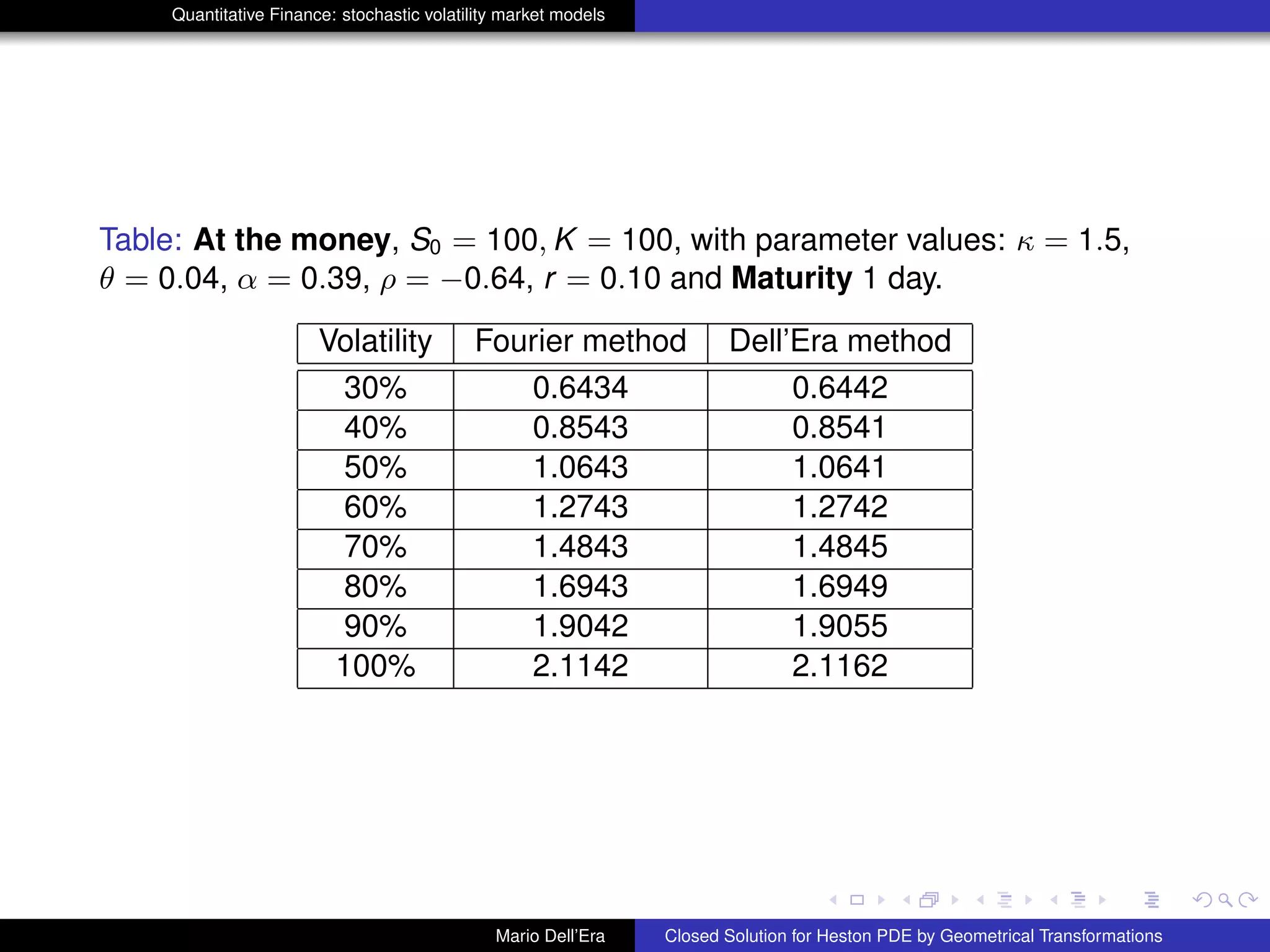
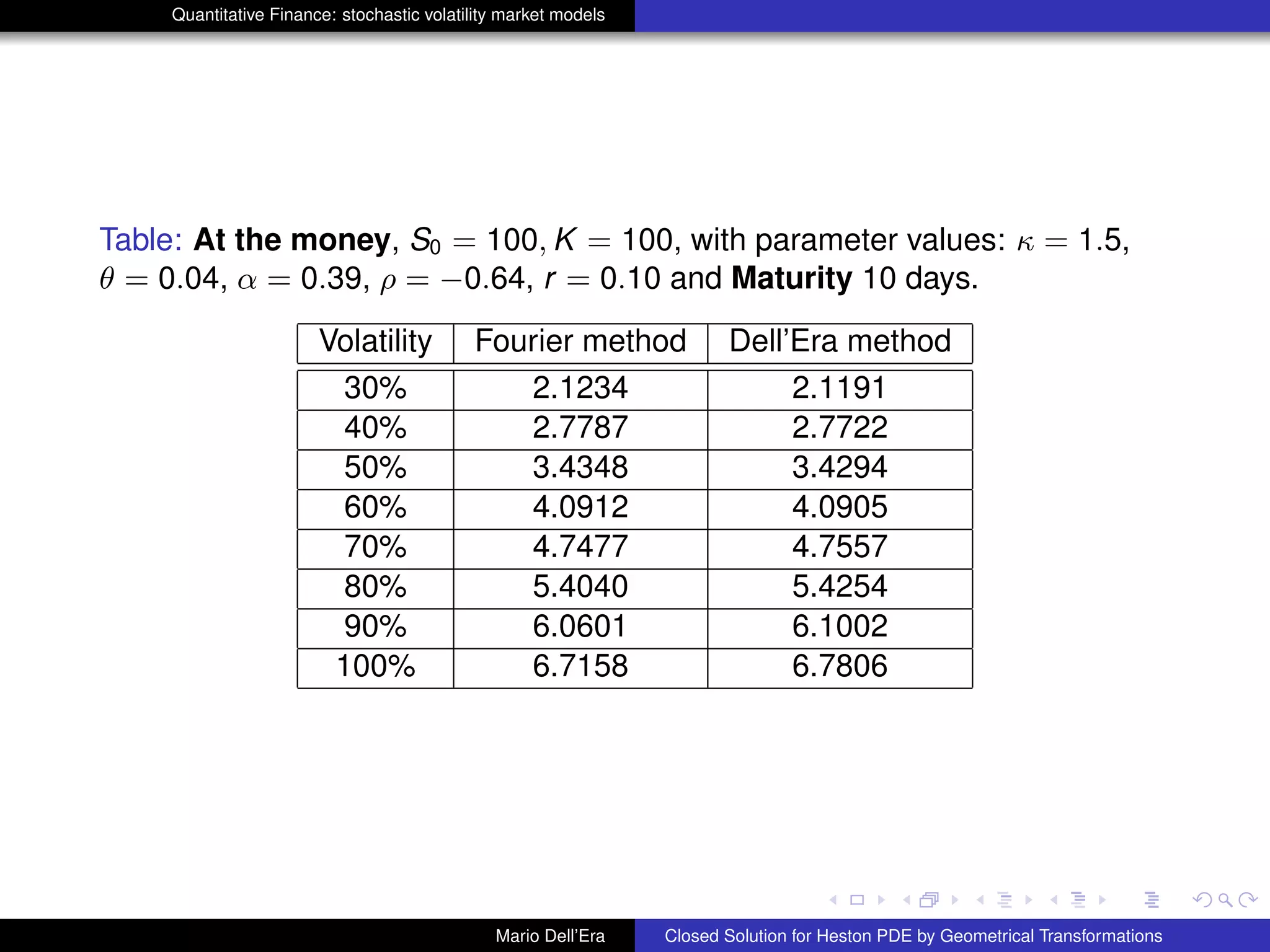
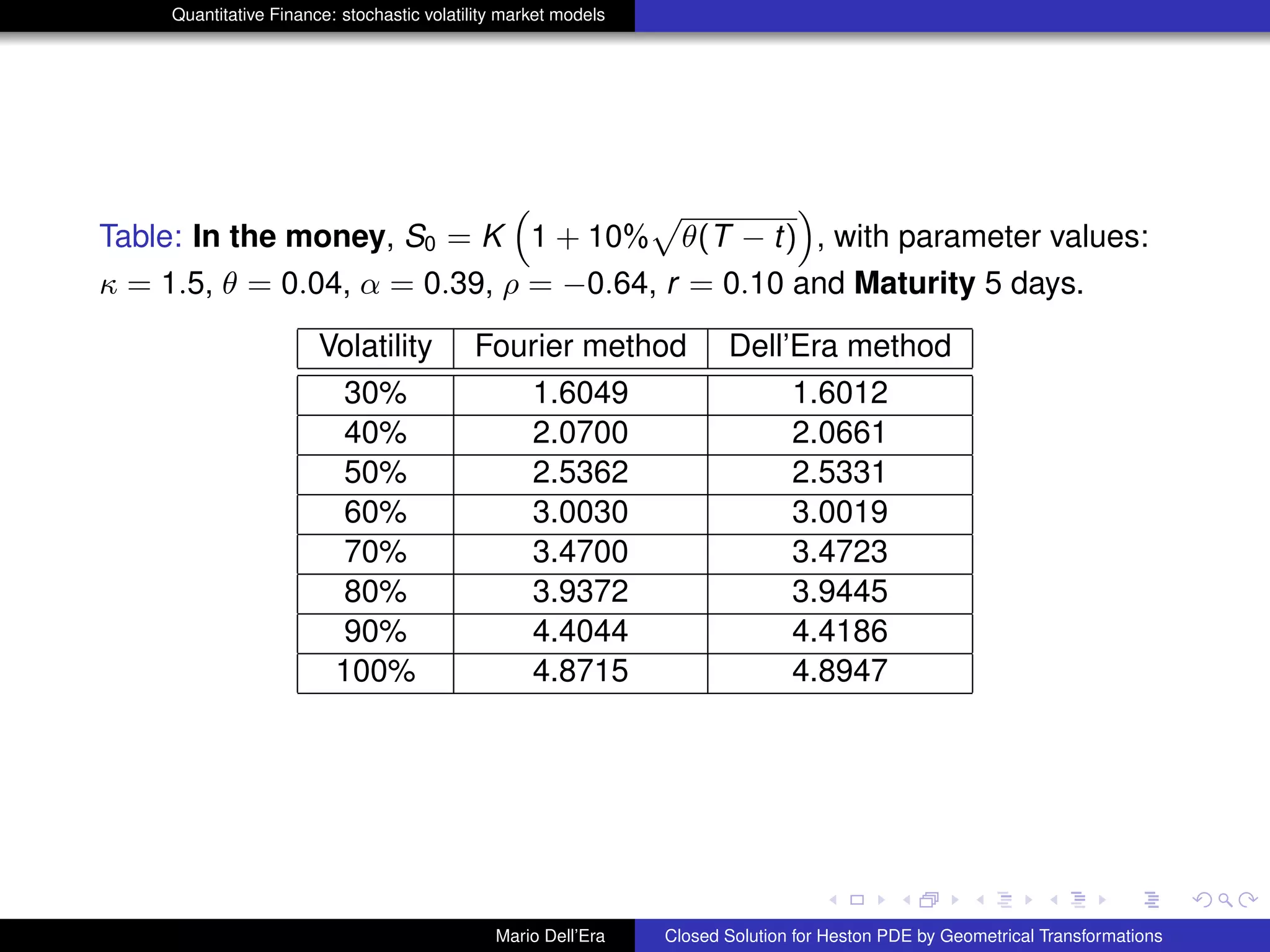
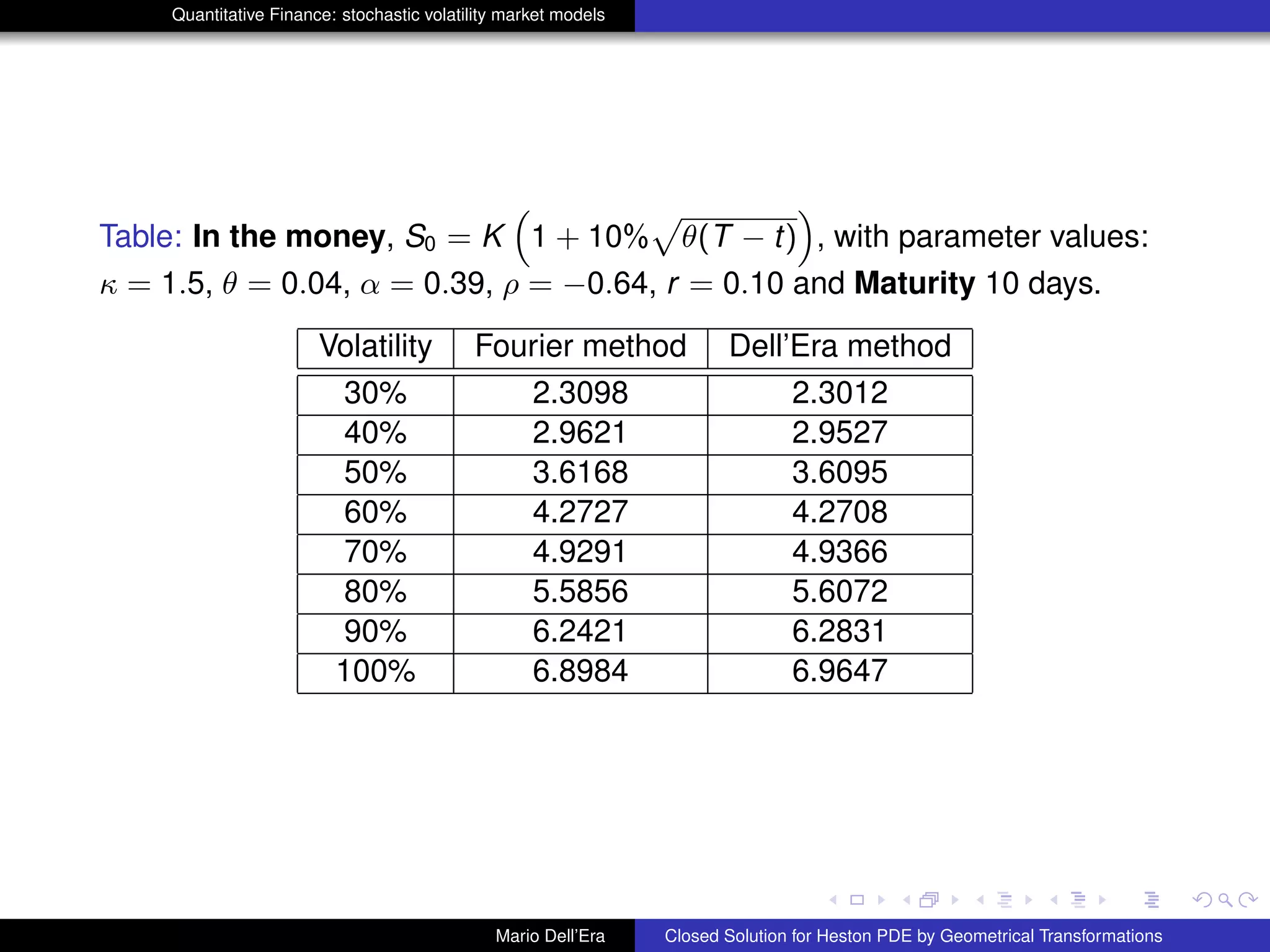
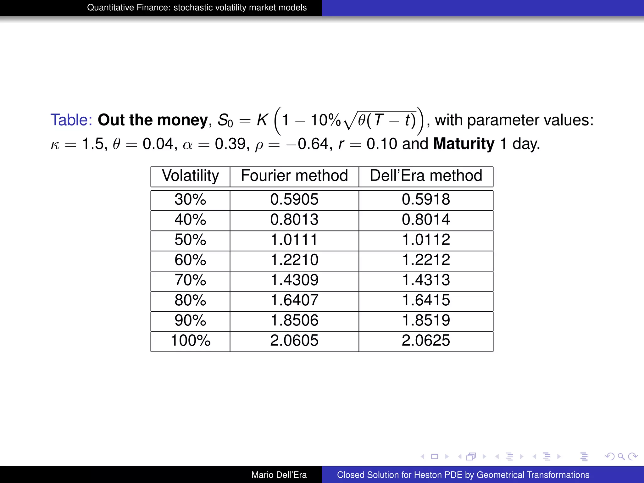
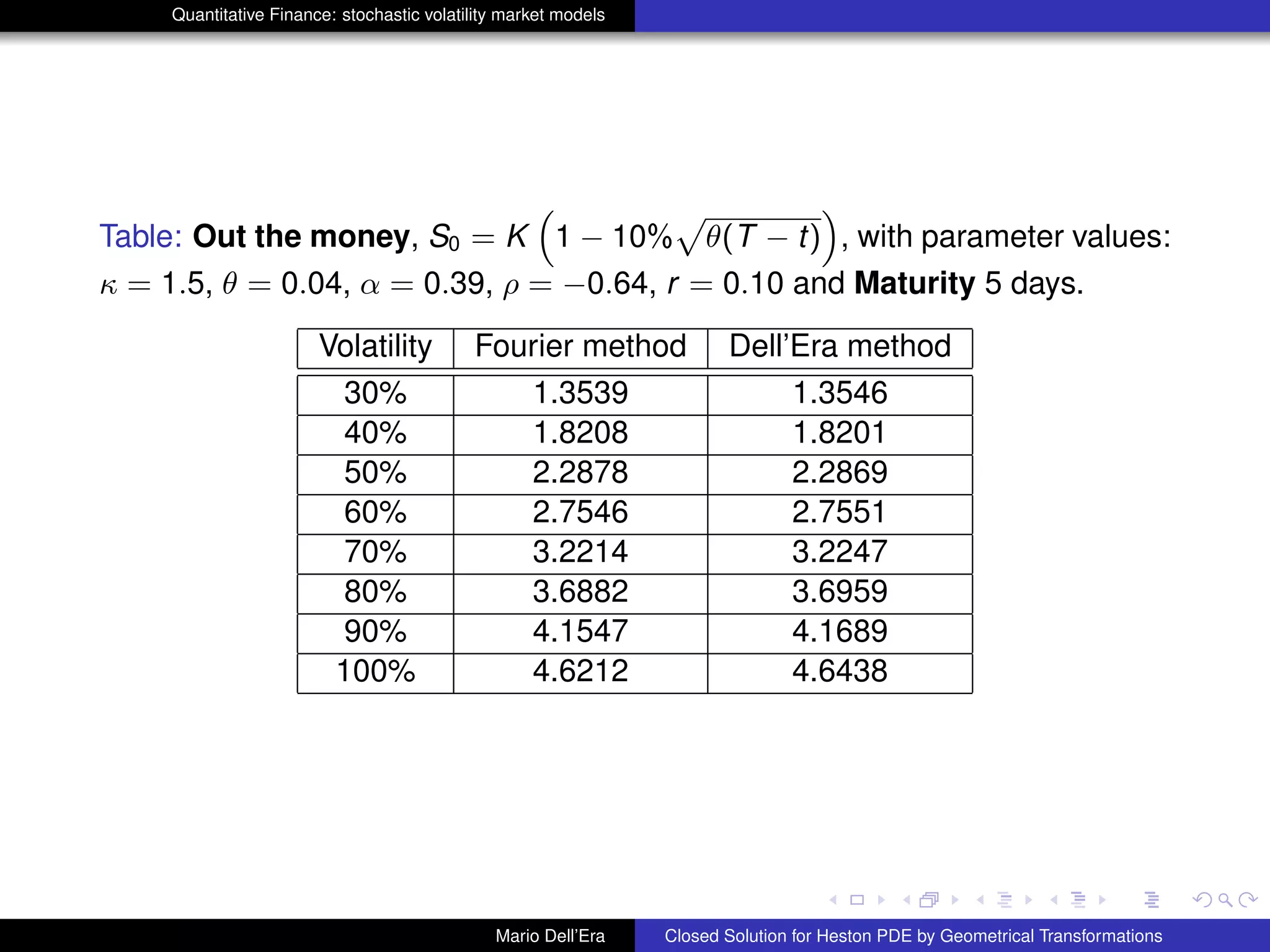
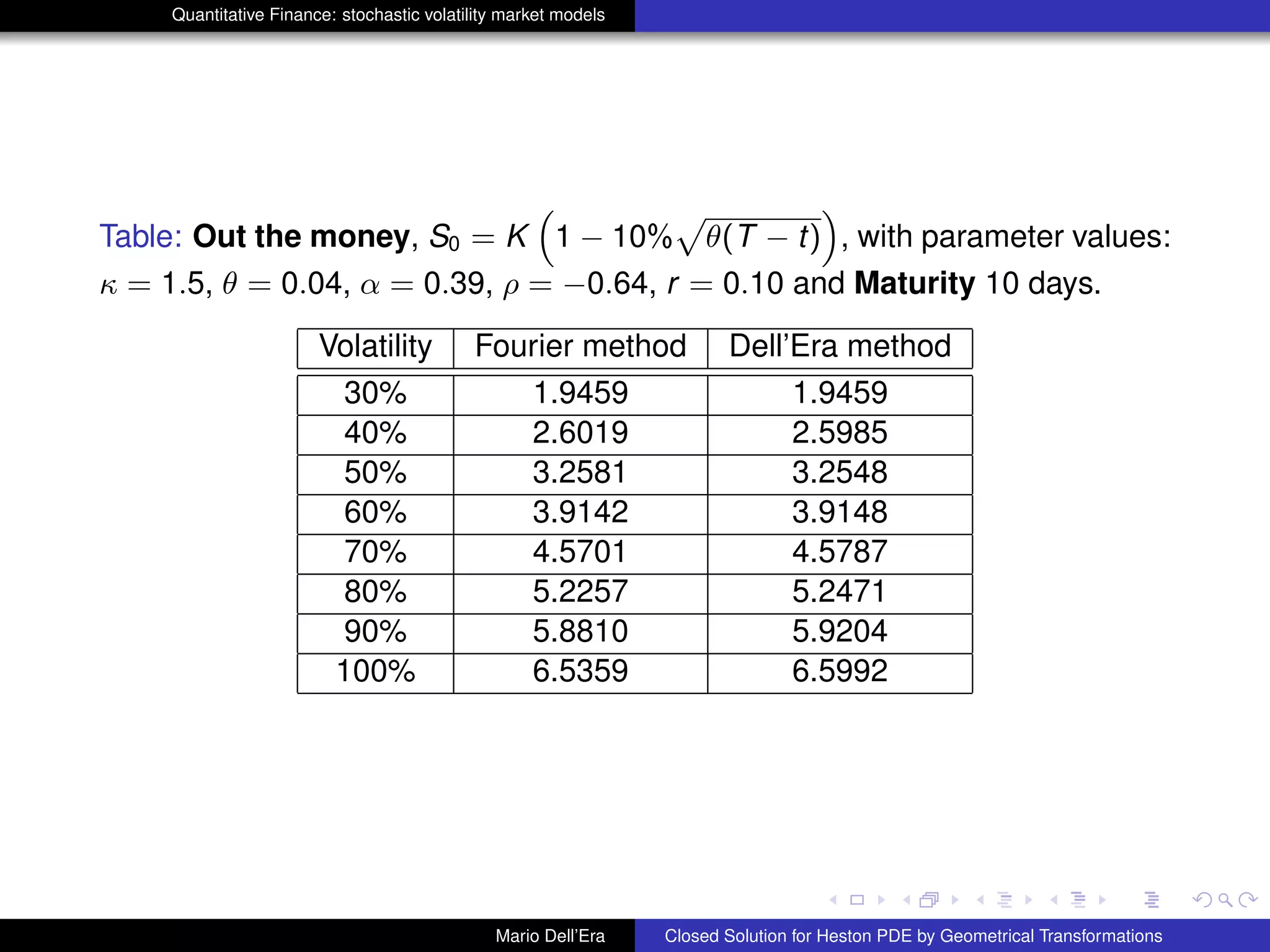
Numerical Validation
The approximation τ → 0 will be here interpreted as option pricing for few
days. From 1 day up to 10 days are suitable maturities to prove our validation
hypothesis, at varying of volatility. Parameter values are those in Bakshi, Cao
and Chen (1997) namely κ = 1.15, Θ = 0.04, α = 0.39 and ρ = −0.64. We
have chosen r = 10% K = 100, and three different maturities T. In what
follows we use the expected value of the variance process EP[νs] instead of
νs in the term
R T
t
νsds. In the tables hereafter one can see the results of
numerical experiments:
Mario Dell’Era Closed Solution for Heston PDE by Geometrical Transformations](https://image.slidesharecdn.com/slide2013-140625155016-phpapp02/75/Workshop-2013-of-Quantitative-Finance-29-2048.jpg)
![Quantitative Finance: stochastic volatility market models
Numerical Validation
The approximation τ → 0 will be here interpreted as option pricing for few
days. From 1 day up to 10 days are suitable maturities to prove our validation
hypothesis, at varying of volatility. Parameter values are those in Bakshi, Cao
and Chen (1997) namely κ = 1.15, Θ = 0.04, α = 0.39 and ρ = −0.64. We
have chosen r = 10% K = 100, and three different maturities T. In what
follows we use the expected value of the variance process EP[νs] instead of
νs in the term
R T
t
νsds. In the tables hereafter one can see the results of
numerical experiments:
Mario Dell’Era Closed Solution for Heston PDE by Geometrical Transformations](https://image.slidesharecdn.com/slide2013-140625155016-phpapp02/75/Workshop-2013-of-Quantitative-Finance-30-2048.jpg)


![Quantitative Finance: stochastic volatility market models
Conclusions
The proposed method is straightforward from theoretical viewpoint and
seems to be promising from that numerical. We reduce the Heston’s PDE in
a simpler, using , in a right order, suitable changing of variables, whose
Jacobian has not singularity points, unless for ρ = ±1. This evidence gives
us the safety that the variables chosen are well defined.
Besides, the idea to use the expected value of the variance process EP[νs],
instead of νt , provides us, in concrete, a closed solution very easy to
compute; and so, we are also able to know what is the error using the
geometric transformation technique; which is equal to the variance of the
variance process νt : Err = EP[(νt − EP[νt ])2
]. While, using Fourier technique
we are not able to know the numeric error directly, but we need to compare
Fourier prices with Monte Carlo prices, for which one can manage the
variance.
We want to remark that the shown technique is independent to the payoff and
therefore, the pricing activities have the same algorithmic complexity for
every derivatives, unlike using Fourier Transform method, for which the
complexity is tied to the payoff.
Mario Dell’Era Closed Solution for Heston PDE by Geometrical Transformations](https://image.slidesharecdn.com/slide2013-140625155016-phpapp02/75/Workshop-2013-of-Quantitative-Finance-40-2048.jpg)
![Quantitative Finance: stochastic volatility market models
Conclusions
The proposed method is straightforward from theoretical viewpoint and
seems to be promising from that numerical. We reduce the Heston’s PDE in
a simpler, using , in a right order, suitable changing of variables, whose
Jacobian has not singularity points, unless for ρ = ±1. This evidence gives
us the safety that the variables chosen are well defined.
Besides, the idea to use the expected value of the variance process EP[νs],
instead of νt , provides us, in concrete, a closed solution very easy to
compute; and so, we are also able to know what is the error using the
geometric transformation technique; which is equal to the variance of the
variance process νt : Err = EP[(νt − EP[νt ])2
]. While, using Fourier technique
we are not able to know the numeric error directly, but we need to compare
Fourier prices with Monte Carlo prices, for which one can manage the
variance.
We want to remark that the shown technique is independent to the payoff and
therefore, the pricing activities have the same algorithmic complexity for
every derivatives, unlike using Fourier Transform method, for which the
complexity is tied to the payoff.
Mario Dell’Era Closed Solution for Heston PDE by Geometrical Transformations](https://image.slidesharecdn.com/slide2013-140625155016-phpapp02/75/Workshop-2013-of-Quantitative-Finance-41-2048.jpg)
![Quantitative Finance: stochastic volatility market models
Conclusions
The proposed method is straightforward from theoretical viewpoint and
seems to be promising from that numerical. We reduce the Heston’s PDE in
a simpler, using , in a right order, suitable changing of variables, whose
Jacobian has not singularity points, unless for ρ = ±1. This evidence gives
us the safety that the variables chosen are well defined.
Besides, the idea to use the expected value of the variance process EP[νs],
instead of νt , provides us, in concrete, a closed solution very easy to
compute; and so, we are also able to know what is the error using the
geometric transformation technique; which is equal to the variance of the
variance process νt : Err = EP[(νt − EP[νt ])2
]. While, using Fourier technique
we are not able to know the numeric error directly, but we need to compare
Fourier prices with Monte Carlo prices, for which one can manage the
variance.
We want to remark that the shown technique is independent to the payoff and
therefore, the pricing activities have the same algorithmic complexity for
every derivatives, unlike using Fourier Transform method, for which the
complexity is tied to the payoff.
Mario Dell’Era Closed Solution for Heston PDE by Geometrical Transformations](https://image.slidesharecdn.com/slide2013-140625155016-phpapp02/75/Workshop-2013-of-Quantitative-Finance-42-2048.jpg)

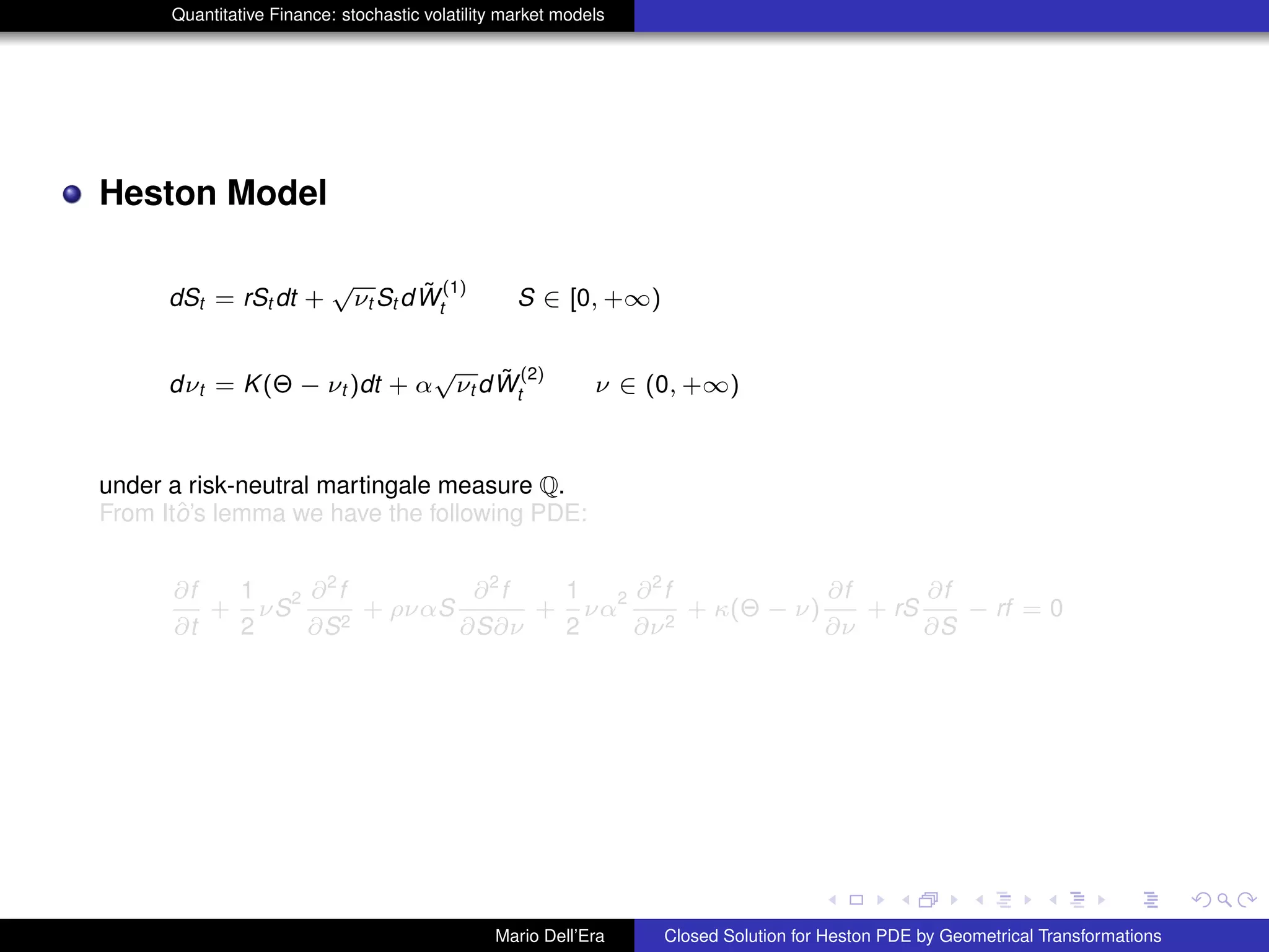
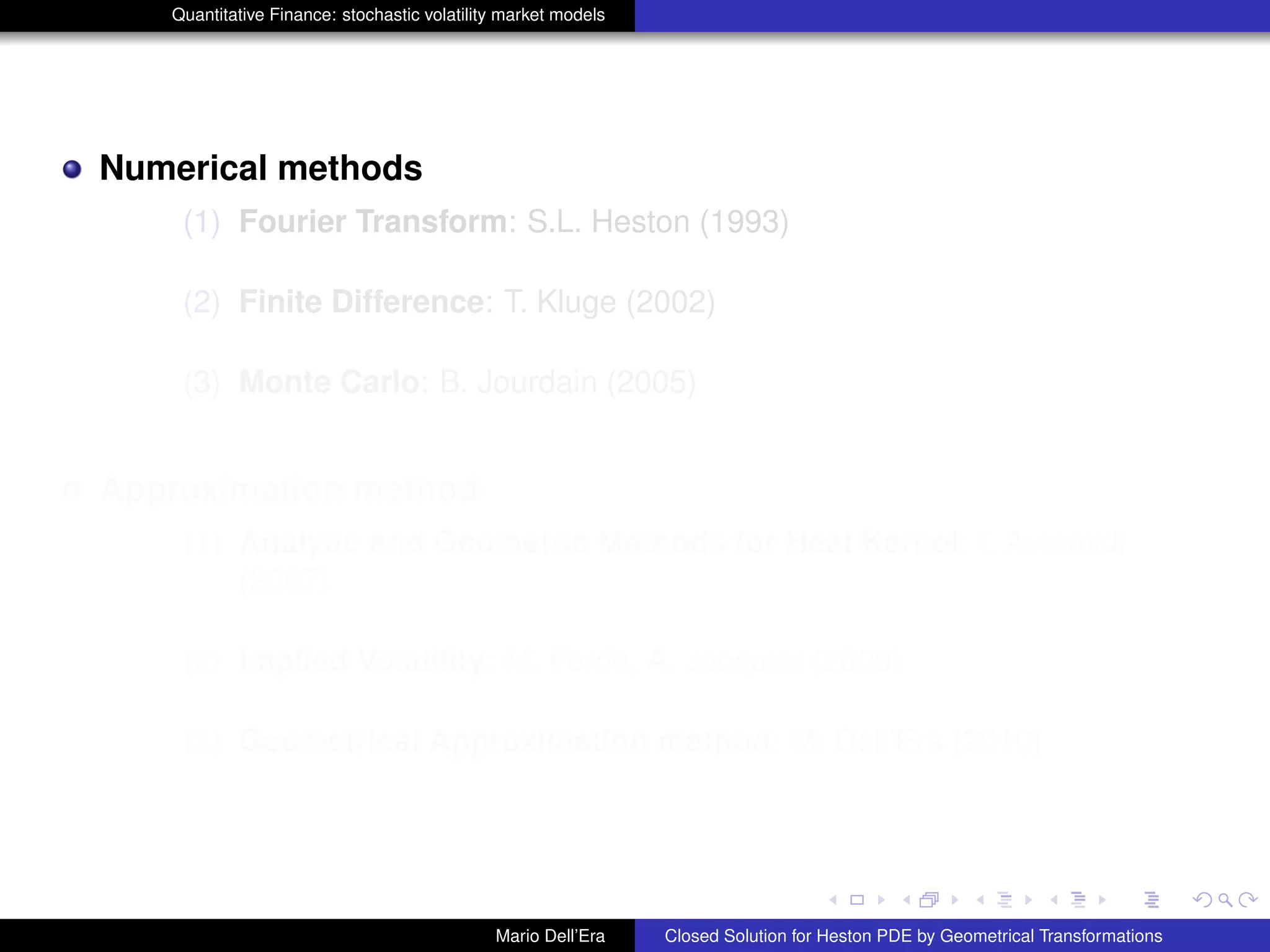
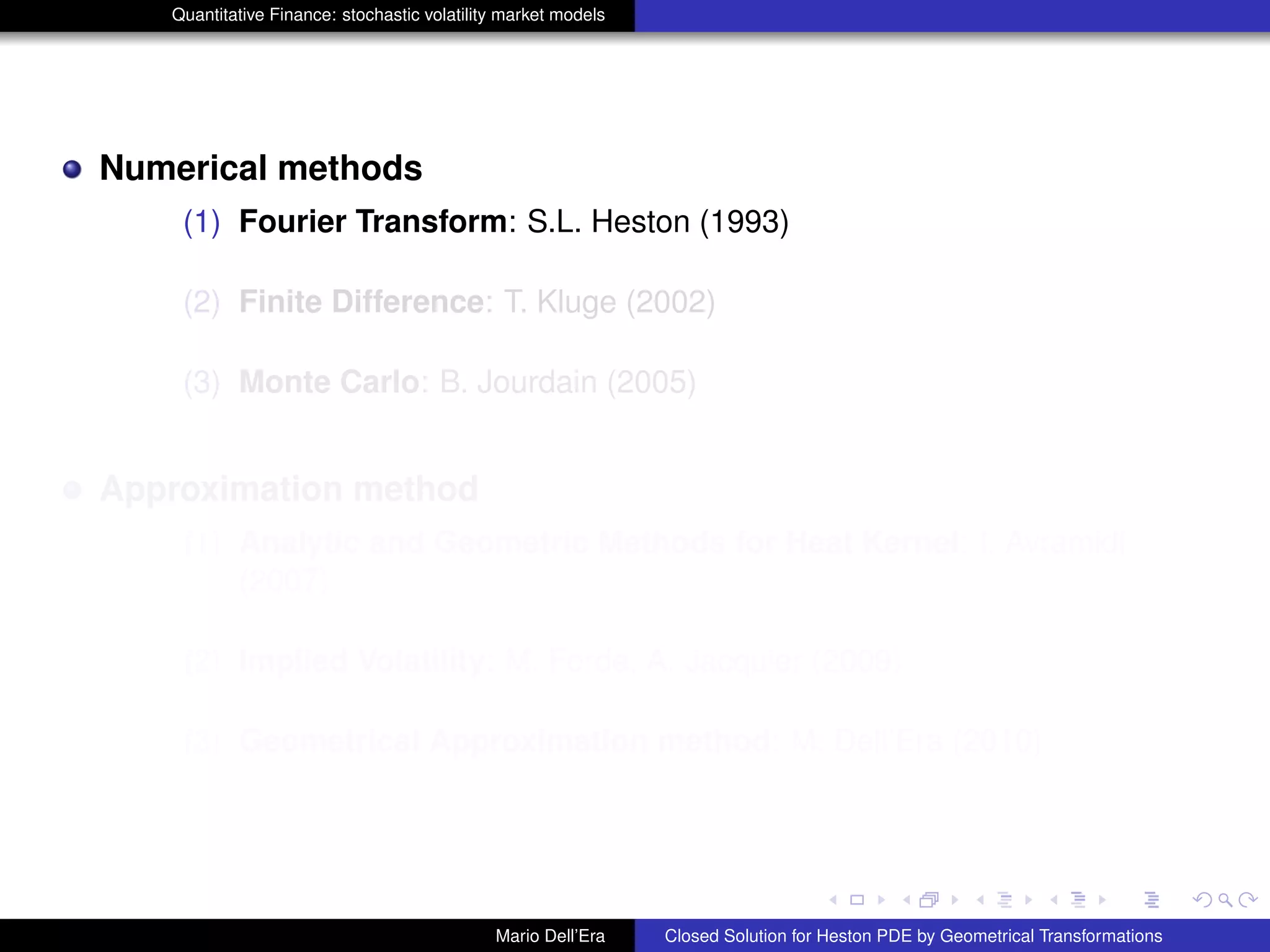
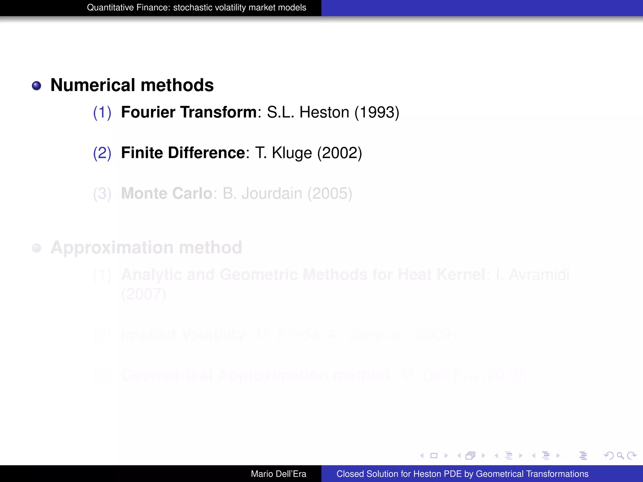
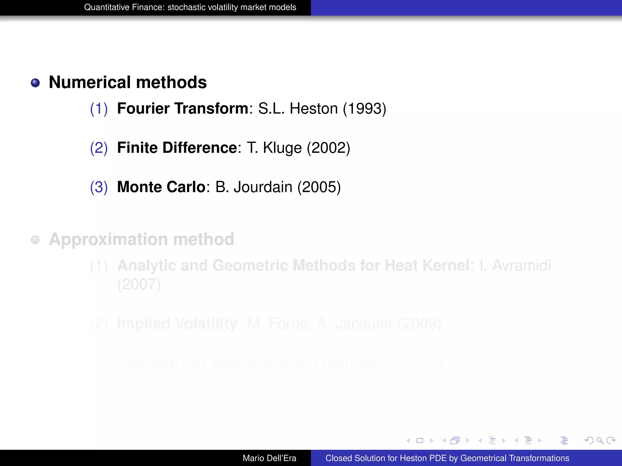
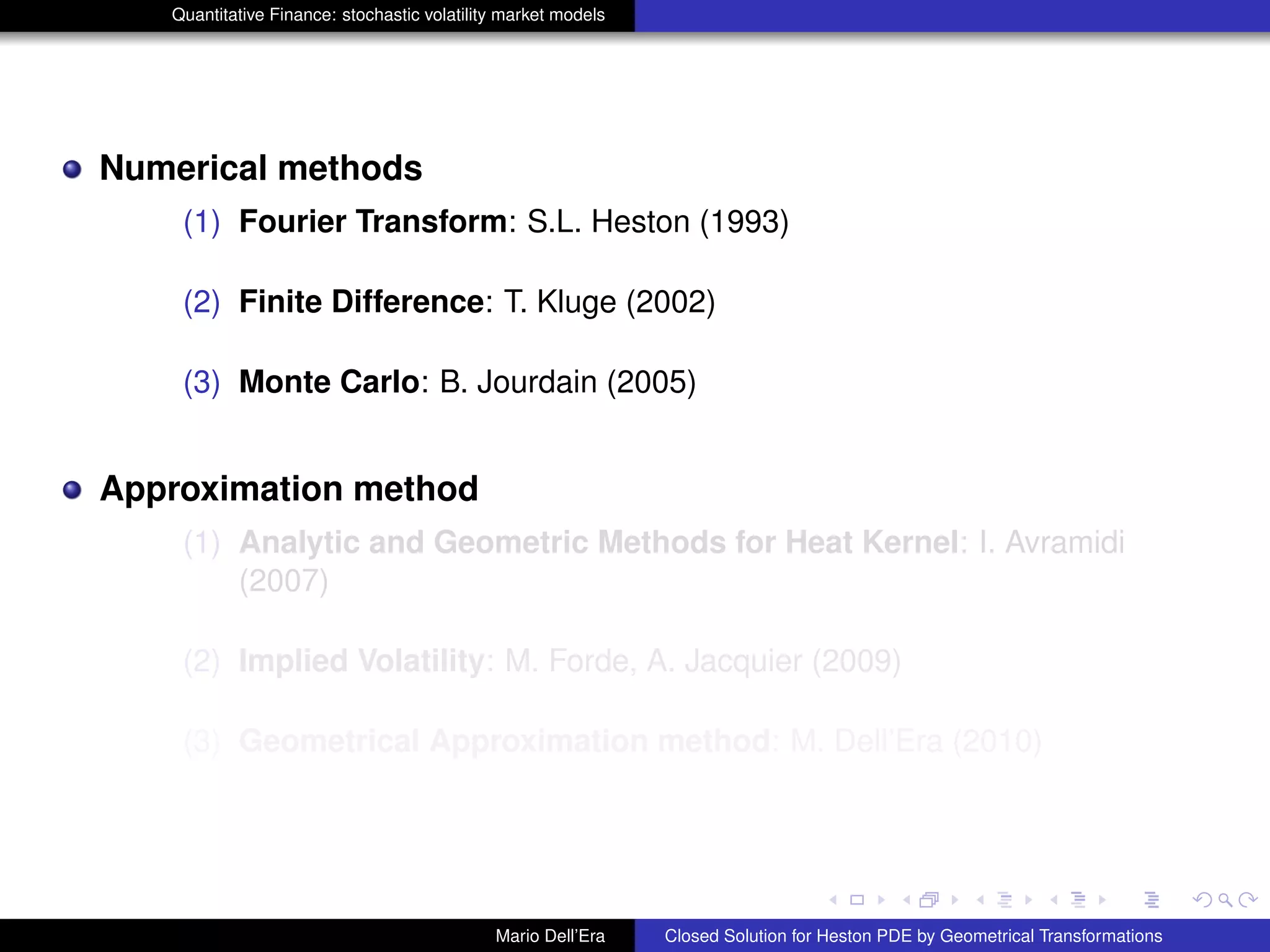
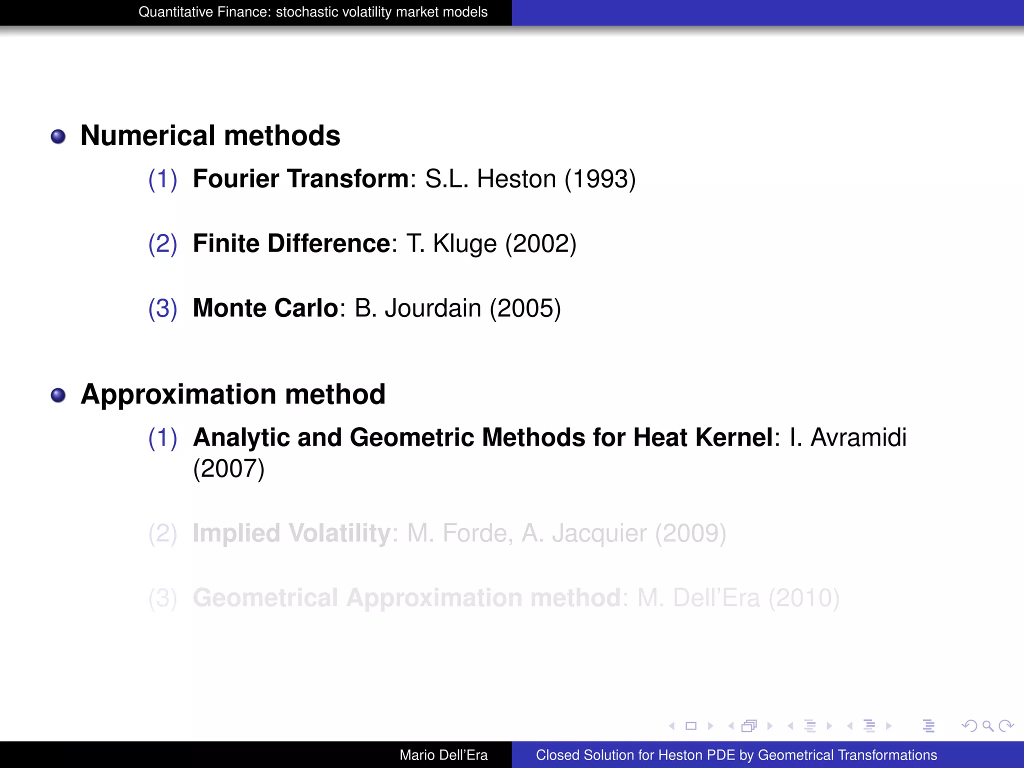
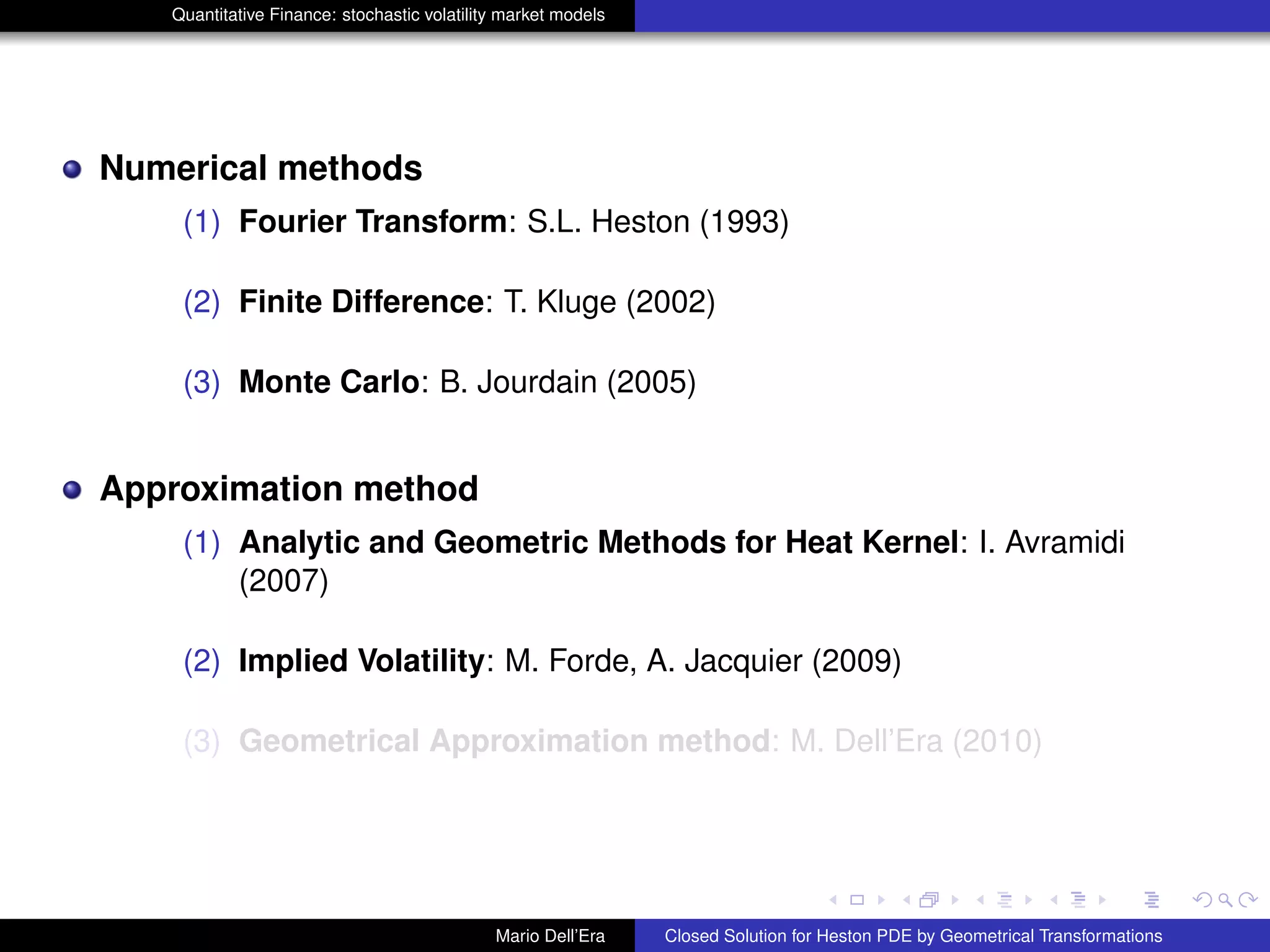
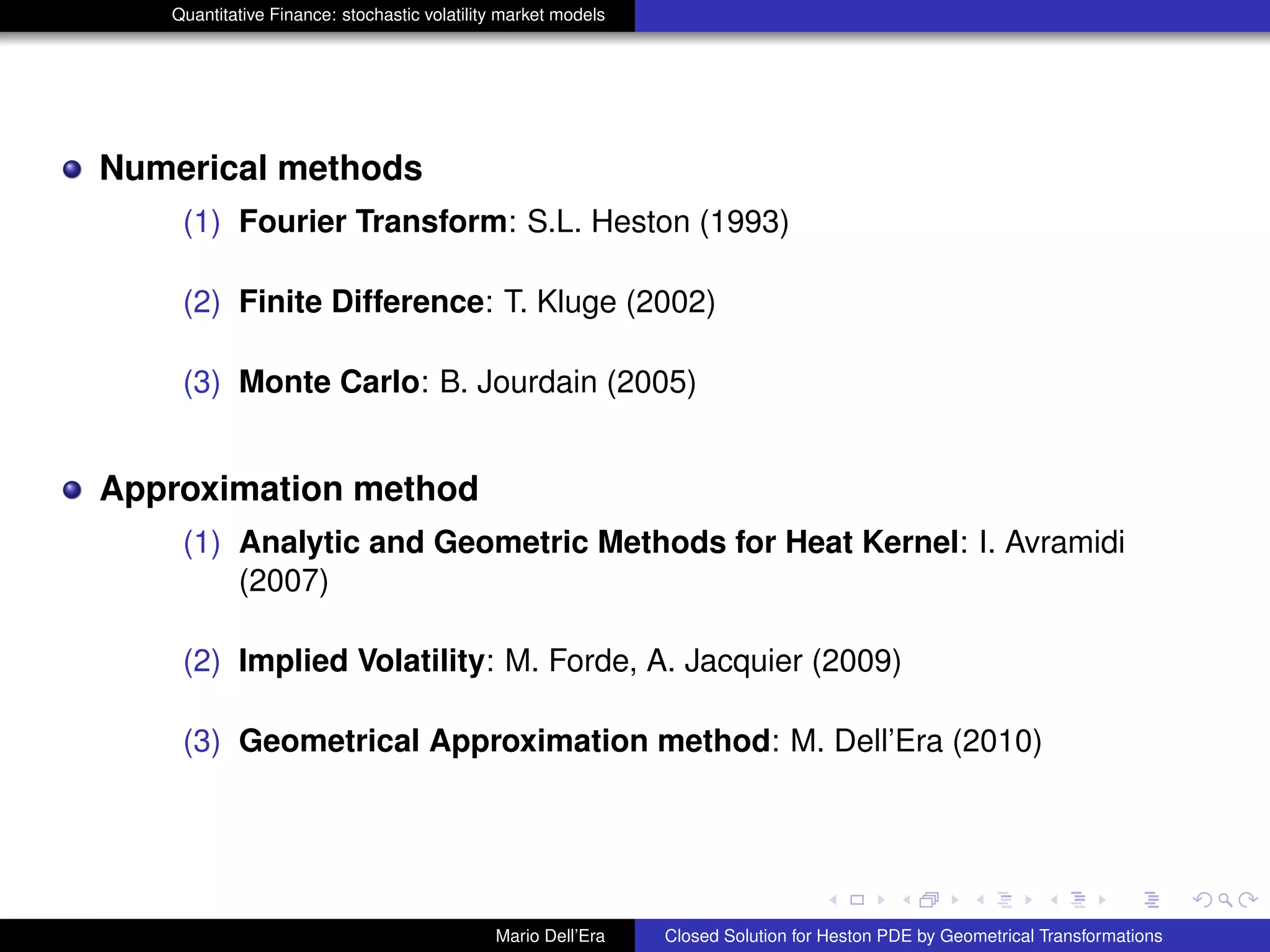
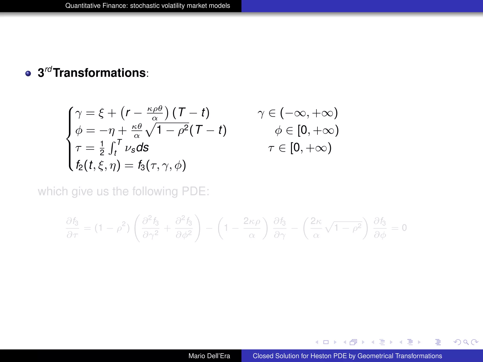
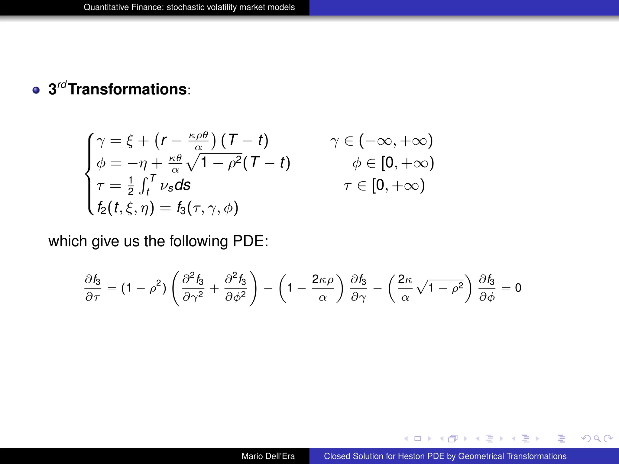
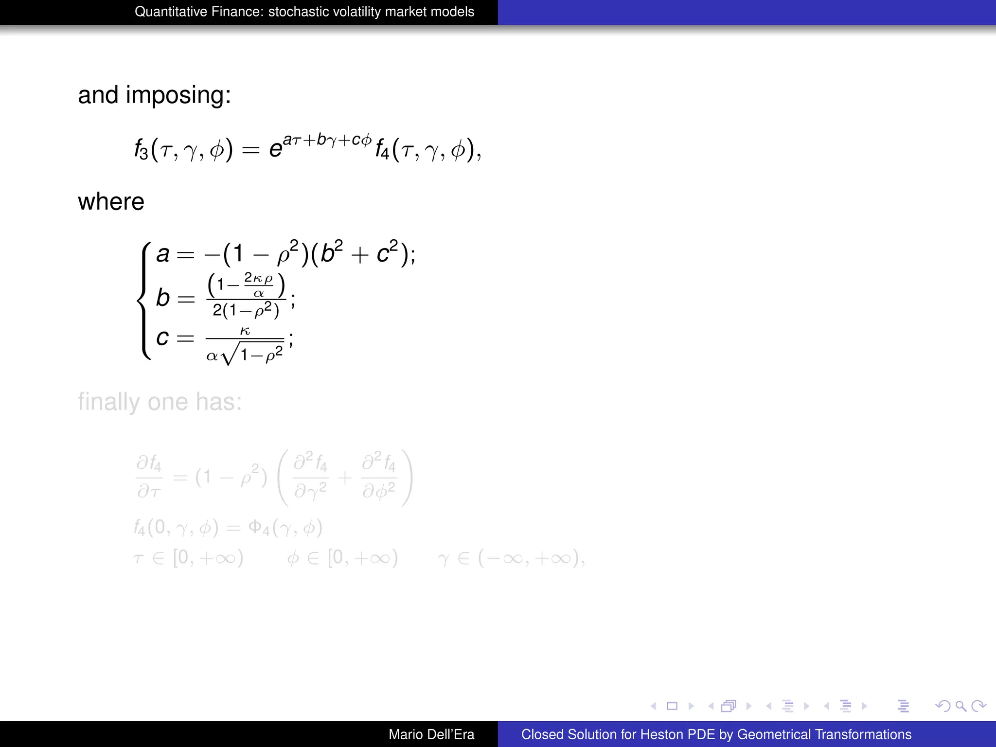
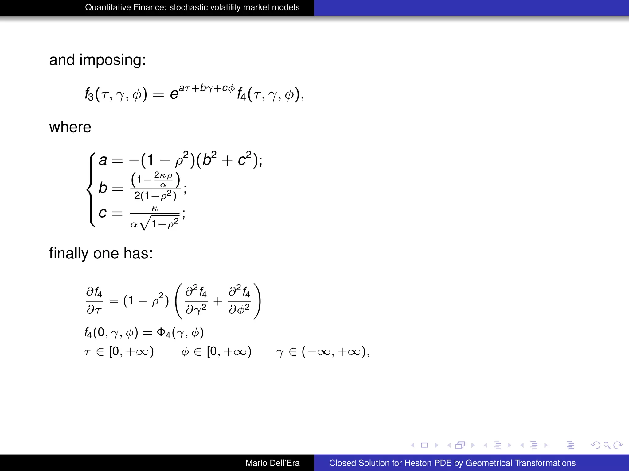
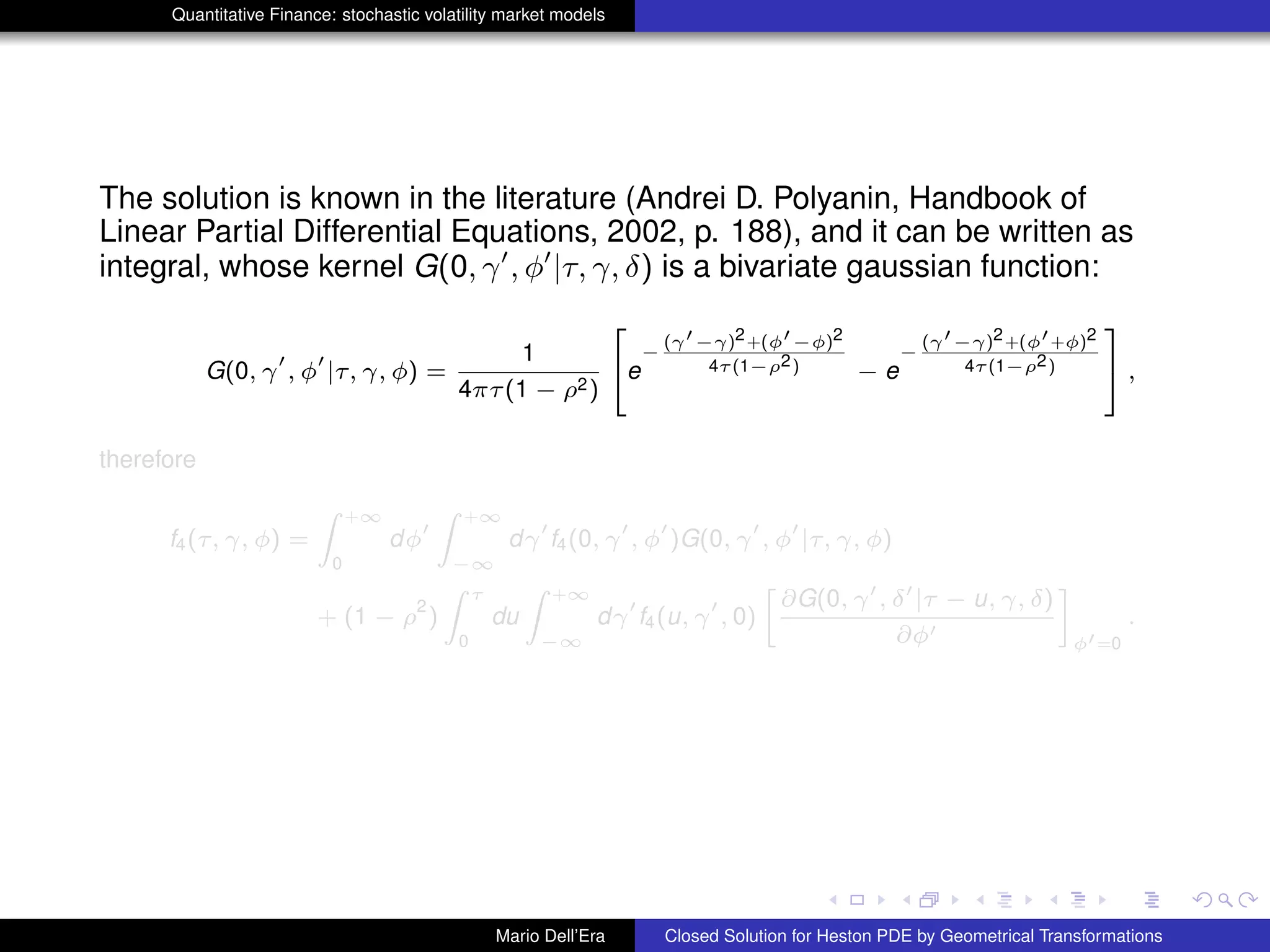
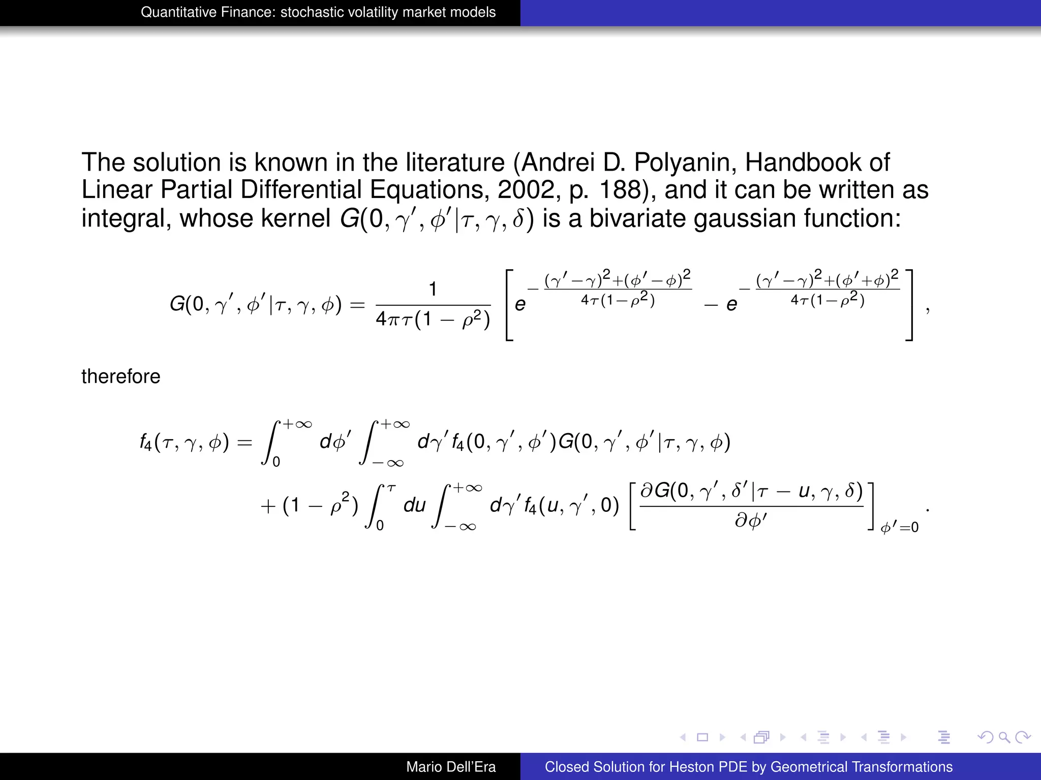
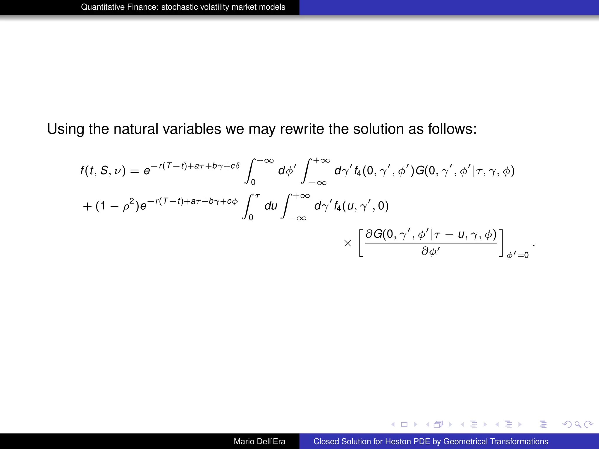
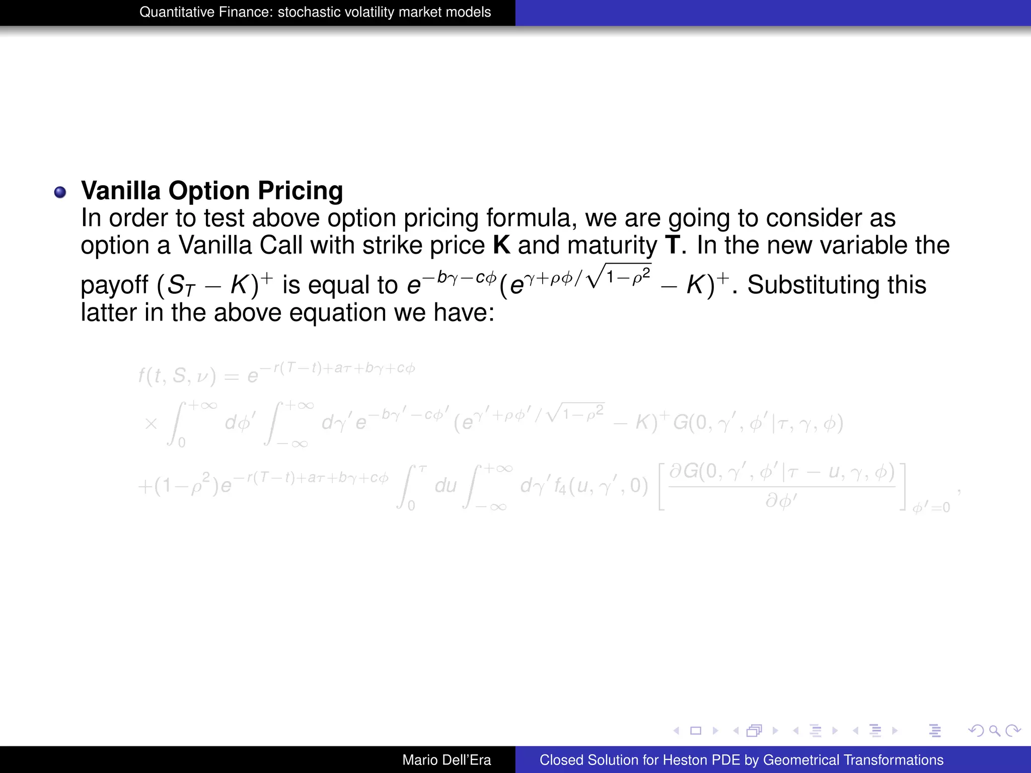
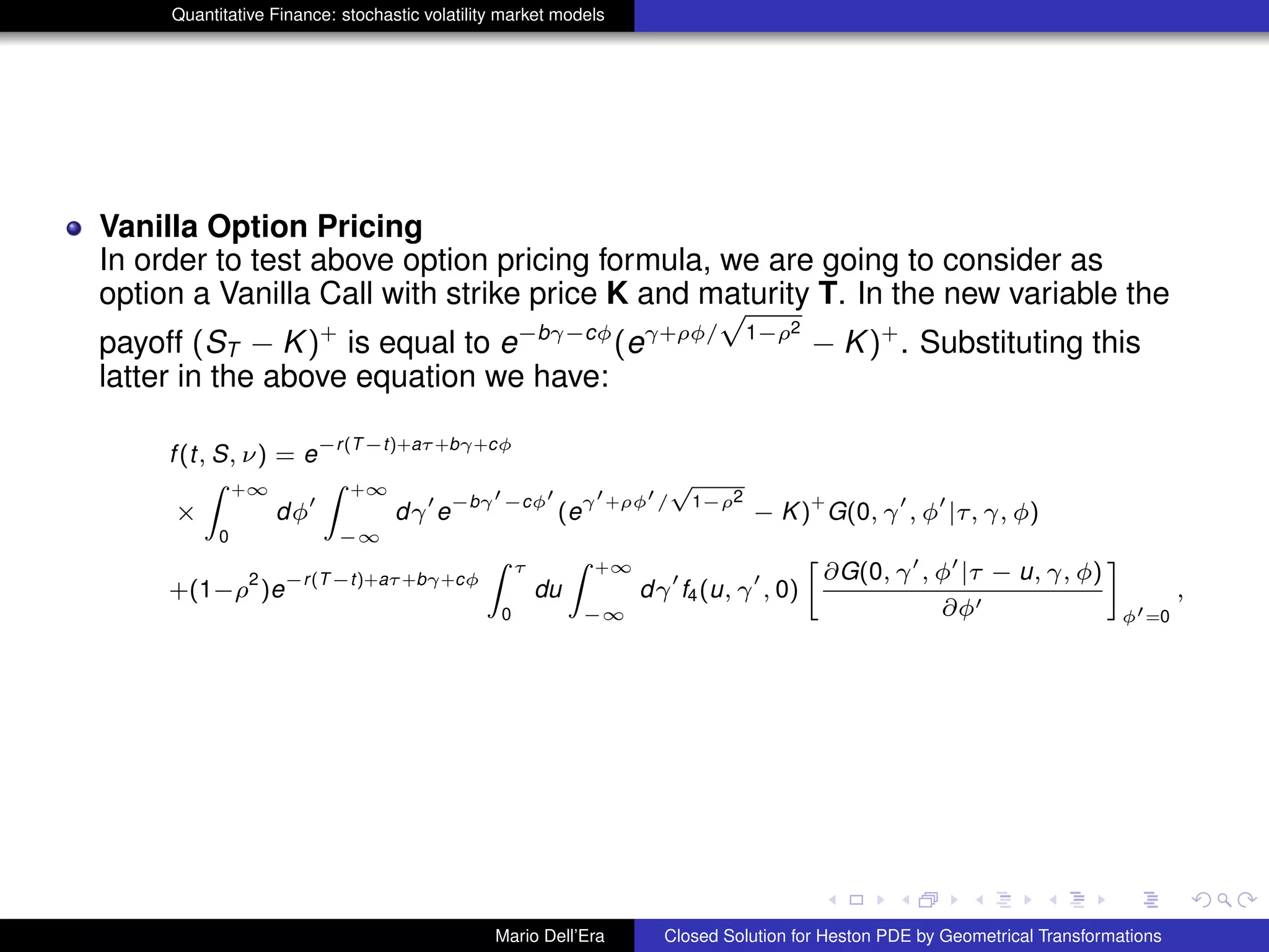
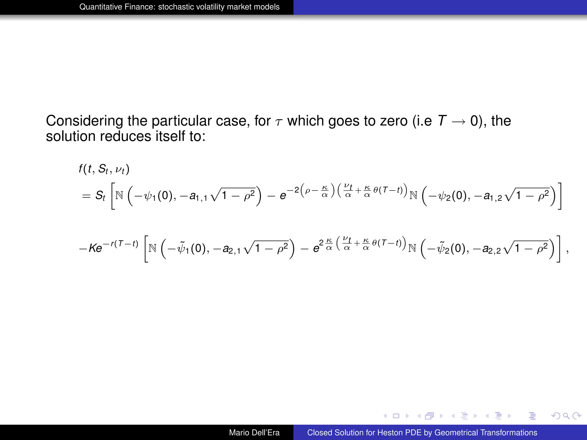
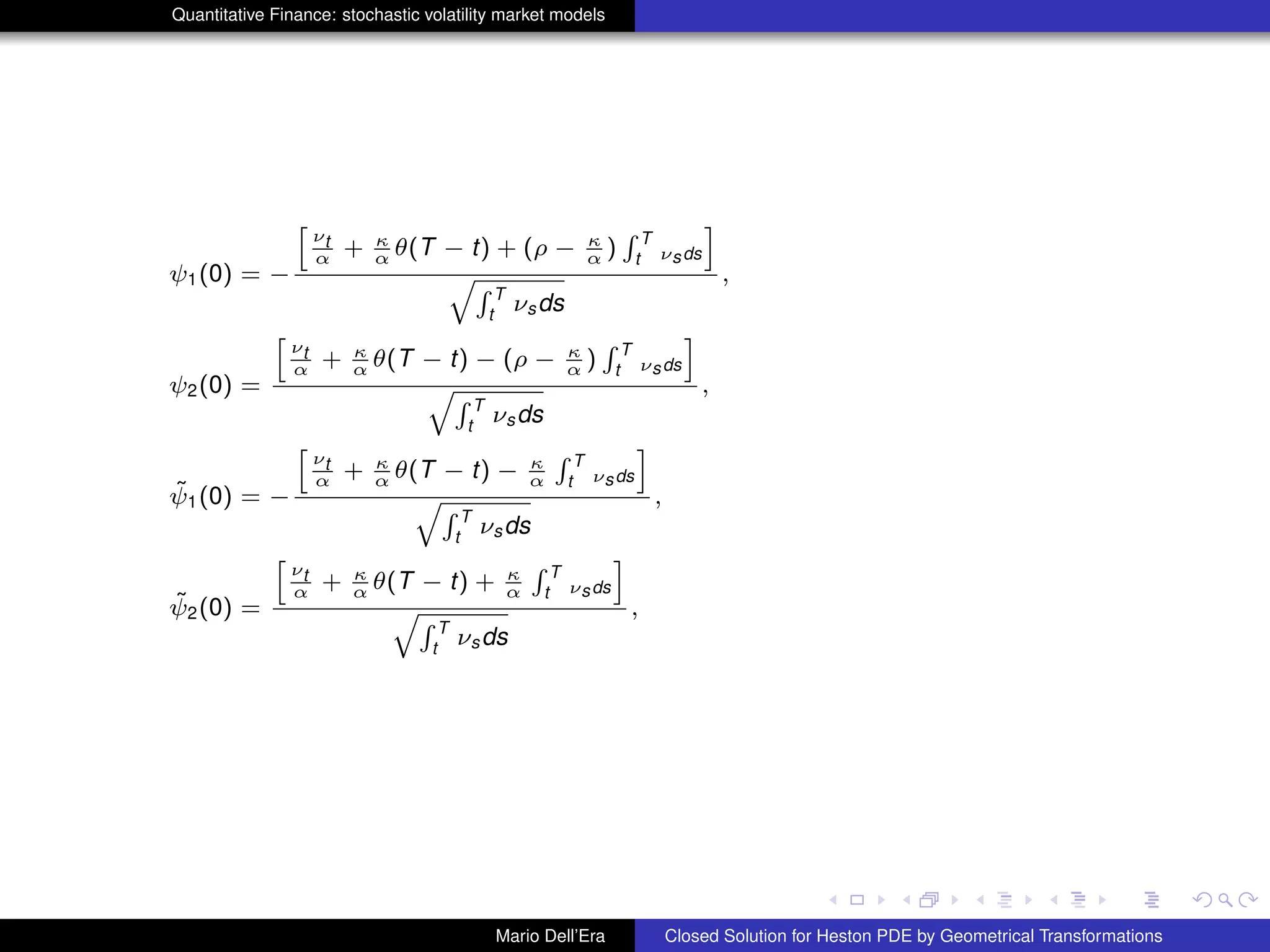
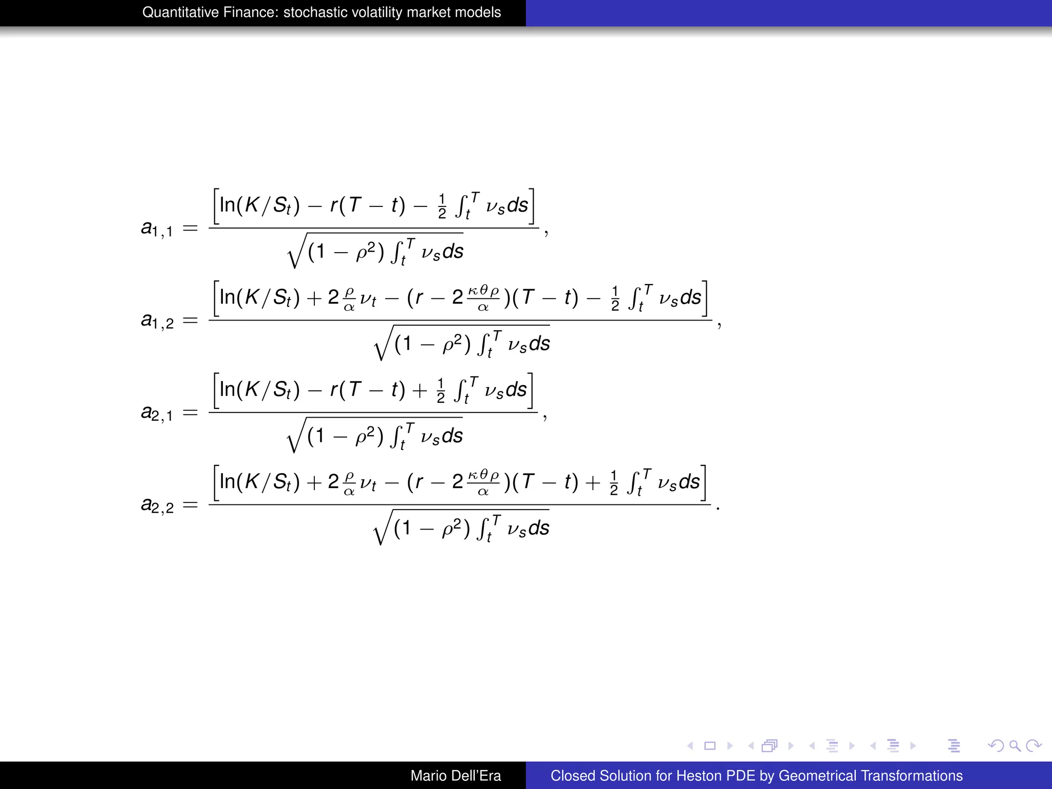
This document summarizes Mario Dell'Era's presentation on finding a closed solution for the Heston PDE using geometrical transformations. It describes the Heston model and the resulting PDE. Existing methods for solving the PDE numerically are outlined. Dell'Era then presents a new methodology using coordinate transformations to solve the PDE, applying three successive transformations to simplify the PDE. This results in an exponential solution for the transformed PDE.