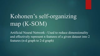
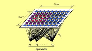
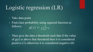
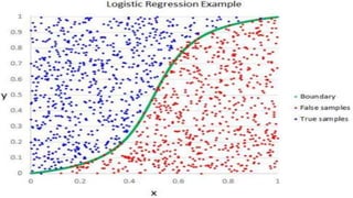
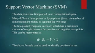
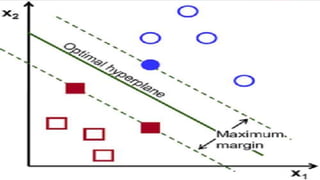
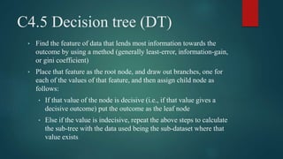
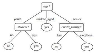
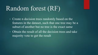
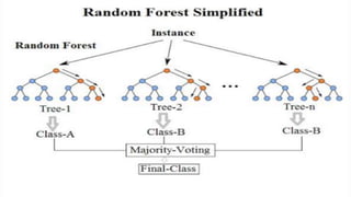
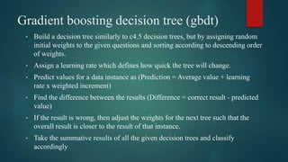
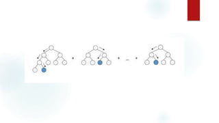
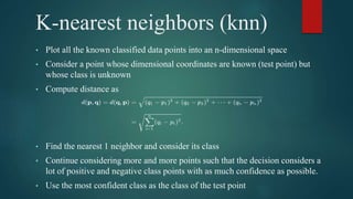
The document discusses several machine learning algorithms: Kohonen's self-organizing map (SOM) which reduces dimensionality; K-means clustering which groups similar data points; logistic regression which classifies data using probabilities; support vector machines (SVM) which find optimal separating hyperplanes; C4.5 decision trees which classify using a question-answer tree structure; random forests which create many decision trees; gradient boosting decision trees which iteratively adjust weights; and K-nearest neighbors (KNN) which classifies based on closest training examples. For each algorithm, it provides a brief overview of the approach and key steps or equations involved.

1. Algorithms
Nikita Kapil

2. Kohonen’s self-organizing
map (K-SOM)
Artificial Neural Network - Used to reduce dimensionality
and effectively represent n features of a given dataset into 2
features (n-d graph to 2-d graph)

3. Kohonen’s Self-Organizing Map (SOM)
• Each node’s weights are initialized
• One vector (instance) from the dataset is taken
• Every node is examined to calculate which one’s weights are most like the input
vector. The winning node is commonly known as the Best Matching
Unit (BMU), given by
• Then the neighborhood of the BMU is calculated. The amount of neighbors
decreases over time.
• The winning weight is rewarded with becoming more like the sample vector.
• The next vector is then taken from the dataset. These steps repeat till all data
points are calibrated.

5. K-Means Clustering (K-MC)
Instance-based lazy learning - Used to cluster data
such that similar data points are represented together
and dissimilar data points are further away.

6. K-means clustering (k-mc)
• For k number of clusters, choose k random data points as centroids of
the clusters.
• Now choose one data point after another (other than the centroid
points) and calculate distance (preferably Euclidean), given by
• Cluster the data point with the nearest centroid and recalculate the
centroid taking mean of coordinates
• Repeat for other data points

8. Logistic Regression (LR)
Instance based quick learning - Used to map dependent
variables to an independent variable and separate the
positive and negative instances.

9. Logistic regression (LR)
• Take data point
• Find class probability using sigmoid function as
follows:
• Then give the data a threshold such that if the value
of g(z) is above that threshold then it is considered
positive (1) otherwise it is considered negative (0)

11. Support Vector machine
(SVM)
Instance-based quick learning - Used to make a
hyperplane that separates the positive and negative
samples with highest amount of margin

12. Support Vector Machine (SVM)
• The data points are first plotted in an n-dimensional space.
• Many different lines, planes or hyperplanes (based on number of
dimensions) are plotted to separate the two cases
• The line/plane/hyperplane is chosen which has a maximum
amount of margin between the positive and negative data points.
This can be represented as
• The above formula can be used to identify positive classes

14. C4.5 decision tree (DT)
Decision Tree based learning - Used for binary classification
(two outcomes) in a question-answer tree format, with most
relevant questions at the top and least relevant questions at
the bottom

15. C4.5 Decision tree (DT)
• Find the feature of data that lends most information towards the
outcome by using a method (generally least-error, information-gain,
or gini coefficient)
• Place that feature as the root node, and draw out branches, one for
each of the values of that feature, and then assign child node as
follows:
• If that value of the node is decisive (i.e., if that value gives a
decisive outcome) put the outcome as the leaf node
• Else if the value is indecisive, repeat the above steps to calculate
the sub-tree with the data used being the sub-dataset where that
value exists

17. Random forest (RF)
Decision Tree based learning - An ensemble model
that creates a lot of random trees and takes majority
vote of their decisions

18. Random forest (RF)
• Create n decision trees randomly based on the
features in the dataset, such that one tree may be a
subset of another but no tree is the exact same
• Obtain the result of all the decision trees and take
majority vote to get the result

20. Gradient boosting decision
tree (GBdt)
Decision Tree based greedy learning - An advanced
decision tree that assigns weights to questions and
calibrates weight to get a maximum accuracy tree.

21. Gradient boosting decision tree (gbdt)
• Build a decision tree similarly to c4.5 decision trees, but by assigning random
initial weights to the given questions and sorting according to descending order
of weights.
• Assign a learning rate which defines how quick the tree will change.
• Predict values for a data instance as (Prediction = Average value + learning
rate x weighted increment)
• Find the difference between the results (Difference = correct result - predicted
value)
• If the result is wrong, then adjust the weights for the next tree such that the
overall result is closer to the result of that instance.
• Take the summative results of all the given decision trees and classify
accordingly

23. K-nearest neighbors (knn)
Instance based lazy learning - Simple, lazy learning
algorithm which classifies the given data points according to
the classes the nearest points.

24. K-nearest neighbors (knn)
• Plot all the known classified data points into an n-dimensional space
• Consider a point whose dimensional coordinates are known (test point) but
whose class is unknown
• Compute distance as
• Find the nearest 1 neighbor and consider its class
• Continue considering more and more points such that the decision considers a
lot of positive and negative class points with as much confidence as possible.
• Use the most confident class as the class of the test point