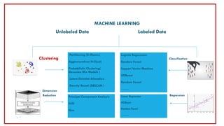
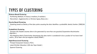
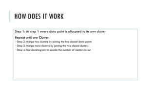
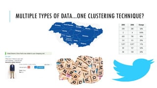
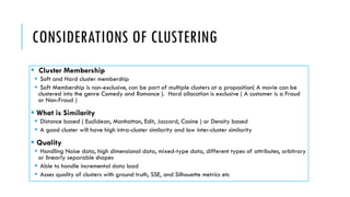
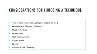
1. Clustering is an unsupervised machine learning technique used to group unlabeled data points into clusters based on similarity. There are several types of clustering including partitioning methods like k-means, hierarchical clustering, density-based clustering, and probabilistic clustering. 2. When choosing a clustering technique, factors to consider include the type of data, whether the number of clusters is known, the presence of noise or missing data, dimensionality of the data, shape of the clusters, and speed/scalability needs. 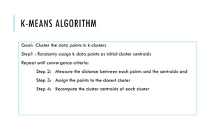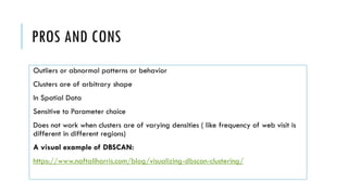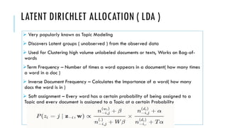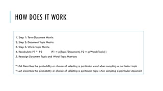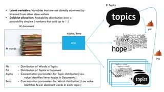3. Popular clustering algorithms include k-means, hierarchical clustering, DBSCAN, Gaussian mixture models, and Latent Dirichlet Allocation (LDA) for text clustering. Each have their own pros and cons depending

1. CLUSTERING
ADP TECH MEETUP
Vidhya Chandrasekaran

2. MACHINE LEARNING
Unlabeled Data Labeled Data
Clustering Classification
Dimension
Reduction Regression
Reg
 `
Partitioning (K-Means)
Agglomerative( H-Clust)
Probabilistic Clustering(
Gaussian Mix Models )
Latent Dirichlet Allocation
Density Based (DBSCAN )
Principal Component Analysis
SVD
tSne
Logistic Regression
Random Forest
Support Vector Machine
XGBoost
Random Forest
……..
Linear Regression
XGBoost
Random Forest
……..

3. WHY CLUSTER?

4. MULTIPLE TYPES OF DATA...ONE CLUSTERING TECHNIQUE?

5. CONSIDERATIONS OF CLUSTERING
▪ Cluster Membership
▪ Soft and Hard cluster membership
▪ Soft Membership is non-exclusive, can be part of multiple clusters at a proposition( A movie can be
clustered into the genre Comedy and Romance ). Hard allocation is exclusive ( A customer is a Fraud
or Non-Fraud )
▪ What is Similarity
▪ Distance based ( Euclidean, Manhattan, Edit, Jaccard, Cosine ) or Density based
▪ A good cluster will have high intra-cluster similarity and low inter-cluster similarity
▪ Quality
▪ Handling Noise data, high dimensional data, mixed-type data, different types of attributes, arbitrary
or linearly separable shapes
▪ Able to handle incremental data load
▪ Asses quality of clusters with ground truth, SSE, and Silhouette metrics etc

6. TYPES OF CLUSTERING
Distance Based Clustering
Partitioning Methods ( K-means, k-medians, K-mediods )
Hierarchical : Agglomerative or Divisive( Agnes, Diana etc )
Density Based Clustering
Clustering based on Density of the data points assuming the data identifies a probabilitic density function ( DBSCAN
)
Probabilistic Clustering
Gaussian Mix Models assumes data to be generated by more than one gaussian( Expectation-Maximization
Algorithm )
Non-Negative Matrix Factorization decomposes the data matrix is considered to be a product of two lower level
matrix , all of them with non-negative values( NNMF )
High-Dimensional Clustering
Principal Component Analysis ( PCA )
Latent Dirichlet Allocation ( LDA aka Topic Model )
Spectral Clustering

7. SOME SIMILARITY MEASURES
Similarity for Numerical variables:
Manhattan distance ( L1 Norm )
Euclidean Distance ( L2 Norm )
Similarity for Categorical or Binary Variables
( Jaccard )
Vector Similarity
(Cosine )

8. DISTANCE BASED

9. K-MEANS ALGORITHM
Goal: Cluster the data points in k-clusters
Step1 : Randomly assign k data points as initial cluster centroids
Repeat until convergence criteria:
Step 2: Measure the distance between each points and the centroids and
Step 3: Assign the points to the closest cluster
Step 4: Recompute the cluster centroids of each cluster

10. K-MEANS ALGORITHM VISUALLY
Goal: Cluster the data points in 3 Clusters
STEP 1: Randomly Allocate k-points as cluster Centroids
STEP 2: Measure the distance between each point to the k-centroids

11. K-MEANS
Step 3: Re-calculate the Cluster centroids
Step 4: Calculate Mean and iterate until stopping conditions or until no re-assignment

12. SHORTCOMINGS
➢ Arbitrary shape support only
➢ Sensitive to outliers and noise
➢ Sensitive to Initialization
➢ Supports only continuous variables only
➢ Needs the number of clusters as input

13. OTHER VARIATIONS
K-mediod
Medioid is a central object that has less average similarity with other objects
Can be used when k-means is influenced by outliers and is not efficient
K-Modes
Clusters categorical data
Uses Frequency metrics as opposed to the distance metrics
K-Median
Uses Median to compute and reassign instead of means
Used when it is data is influenced by outliers

14. HIERARCHICAL

15. HIERARCHICAL CLUSTERING
➢ Creates an hierarchy of clusters
➢ Need not pass on the number of clusters as in k-means
➢ Dendrogram can be used to define the number of clusters needed
➢ Bottom-up Hierarchical starts with one large clusters and merge( Agglomerative )
➢ Top-Down Hierarchical Starts with one cluster for each point and divides( Divisive )

16. HOW DOES IT WORK
Step 1: At step 1 every data point is allocated to its own cluster
Repeat until one Cluster:
 Step 2: Merge two clusters by joining the two closest data points
 Step 3: Merge more clusters by joining the two closest clusters
 Step 4: Use dendrogram to decide the number of clusters to cut

17. A Dendrogram
Shortcomings
Resource Intensive
Time consuming
Once the clusters or merged or partitioned can be undone
How does it Split or Merge
Single Link ( Nearest Neighbor )
Local in Behavior
Sensitive to Outliers
Complete Link ( Diameter )
Non-Local in Behavior
Sensitive to Outliers
Average Link ( group average )
Resource intensive
Wards Criterion ( Minimum variance )

18. DENSITY BASED

19. DBSCAN – DENSITY BASED MODEL
➢ Assumes data is drawn from a Probability density Function ( pdf )
➢ Discovers clusters of arbitrary shapes
➢ Spatial data with noise
➢ Groups points together with high density
➢ Parameters:
* Eps(radius): Minimum distance between
two points
* minPoints: Minimum number of points to form a dense region
➢ Each point are considered Core point or Border Point or Outlier

20. DBSCAN IN ACTION
* Image courtesy - Medium

21. PROS AND CONS
Outliers or abnormal patterns or behavior
Clusters are of arbitrary shape
In Spatial Data
Sensitive to Parameter choice
Does not work when clusters are of varying densities ( like frequency of web visit is
different in different regions)
A visual example of DBSCAN:
https://www.naftaliharris.com/blog/visualizing-dbscan-clustering/

22. PROBABILISTIC MODELS Gaussian Mixture Models -
Expectation Maximization

23. GAUSSIAN MIXTURE MODEL
• Assumes data is generated by multiple
Gaussian
• Central Limit theorem supports as the data
size increases, the distribution is usually
Gaussian
• Used when we have Missing variables or
unobserved data. This is central to the EM
Algorithm
• Advantages: Soft assignments, latent
variables
• Disadvantages: Has a Local maxima( saddle
point) problem and re-initializing with
random parameters can help

24. GMM - EM
Gaussian Equation
Mixture of Gaussians
Expectation
Using the current random assignment of mean and covariance, we calculate probabilities for
each Gaussian ( Each data point is generated from one Gaussian).
Maximization:
Using the mean, covariance and weights until convergence

25. EXPECTATION-MAXIMATION
Expectation
Maximization
To update weight: Sum of probability / N
To update weight: mean of all points weighted by the prob that it
Is generated from Gaussian j
To update weight: Co-variance of all points weighted by the
Probability that that point is generated from Gaussian j

26. E-M WITH SIMPLE EXAMPLE - COIN TOSES
Data generated from 2 Coins, 10 Tosses, 5 Trials, 2 Events
H H T T H H T H T T
H H H H H T H H H H
H T H H H H H T H H
H T H T T T H H T T
T H H H T H H H T H

27. WORKING OUT…
Random Assignment: Wa = 0.60, Wb = 0.5
Step 1: Calculate Likelihood
Likelihood of A: Wa h* (1- wa ) n-h = 0.0007962 ( 45% after normalizing )
Likelihood of B: Wb h * (1-wb ) n-h = 0.0009765 ( 55% after normalizing )
Step 2: E-Step: ( For every run ):
“A”:H = 0.45 * 5 = 2.2 Heads
“B”:H = 0.55 * 5 = 2.8 Heads
Step 3: M-Step ( Compute New Weights)
Wa = H/(H+T ) = (21.3)/(21.3+8.6) = 0.71
Wb = H/(H+T ) = (11.7)/(11.7+8.4) = 0.58
Coin A:H Coin B:H
2.2 2.8
7.2 1.8
5.9 2.1
1.4 2.6
4.5 2.5
21.3 11.7

28. DIMENSION REDUCTION Latent Dirichlet Allocation

29. LATENT DIRICHLET ALLOCATION ( LDA )
➢ Very popularly known as Topic Modeling
➢ Discovers Latent groups ( unobserved ) from the observed data
➢ Used for Clustering high volume unlabeled documents or texts, Works on Bag-of-
words
➢Term Frequency – Number of times a word appears in a document( how many times
a word in a doc )
➢ Inverse Document Frequency – Calculates the Importance of a word( how many
docs the word is in )
➢ Soft assignment – Every word has a certain probability of being assigned to a
Topic and every document is assigned to a Topic at a certain Probability

30. HOW DOES IT WORK
1. Step 1: Term-Document Matrix
2. Step 2: Document Topic Matrix
3. Step 3: Word-Topic Matrix
4. Recalculate P1 * P2 (P1 = p(Topic/Document), P2 = p(Word/Topic) )
5. Reassign Document Topic and Word-Topic Matrices
* LDA Describes the probability or chance of selecting a particular word when sampling a particular topic
* LDA Describes the probability or chance of selecting a particular topic when sampling a particular document

31. LDA
M document
N words
K Topics
Phi - Distribution of Words in Topics
Psi - Distribution of Topics in Document
Alpha - Concentration parameters for Topic distribution( Low
value identifies fewer topics in Documents )
Beta - Concentration parameters for Word distribution ( Low value
identifies fewer dominant words in each topic )
• Latent variables: Variables that are not directly observed by
inferred from other observations
• Dirichlet allocation: Probability distribution over a
probability simplex ( numbers that add up to 1 )
Phi
psi
Alpha, Beta

32. CONSIDERATIONS FOR CHOOSING A TECHNIQUE
➢ Type of data ( numerical , categorical, text, binary )
➢ Knowledge of Number of clusters
➢ Noise in the data
➢ Missing data
➢ High dimensionality
➢ Cluster shape
➢ Speed
➢ Column or Row Clustering

33. NEXT STEPS: EXPLORE
Learn other important approaches
Non Negative Matrix Factorization ( NNMF )
Spectral Clustering
Compare clustering approaches visually for your applications
http://education.knoweng.org/clustereng/#
Enrich Knowledge
Data Clustering – Algorithmn snad Application – Charu Aggarwal

34. Q/A