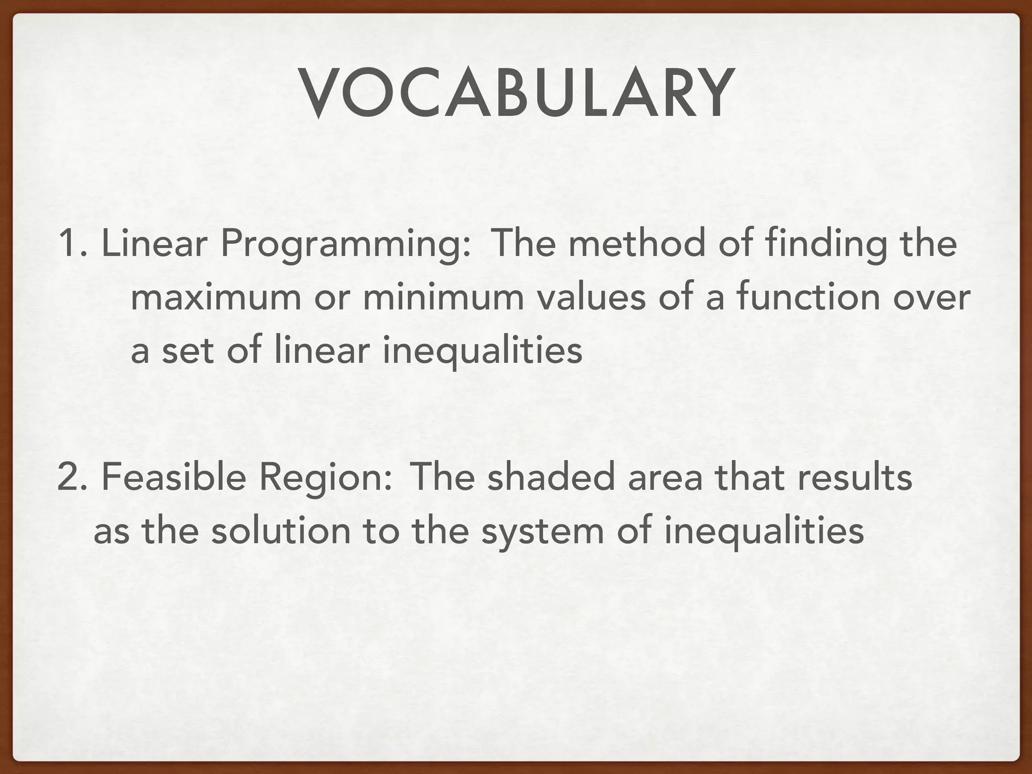
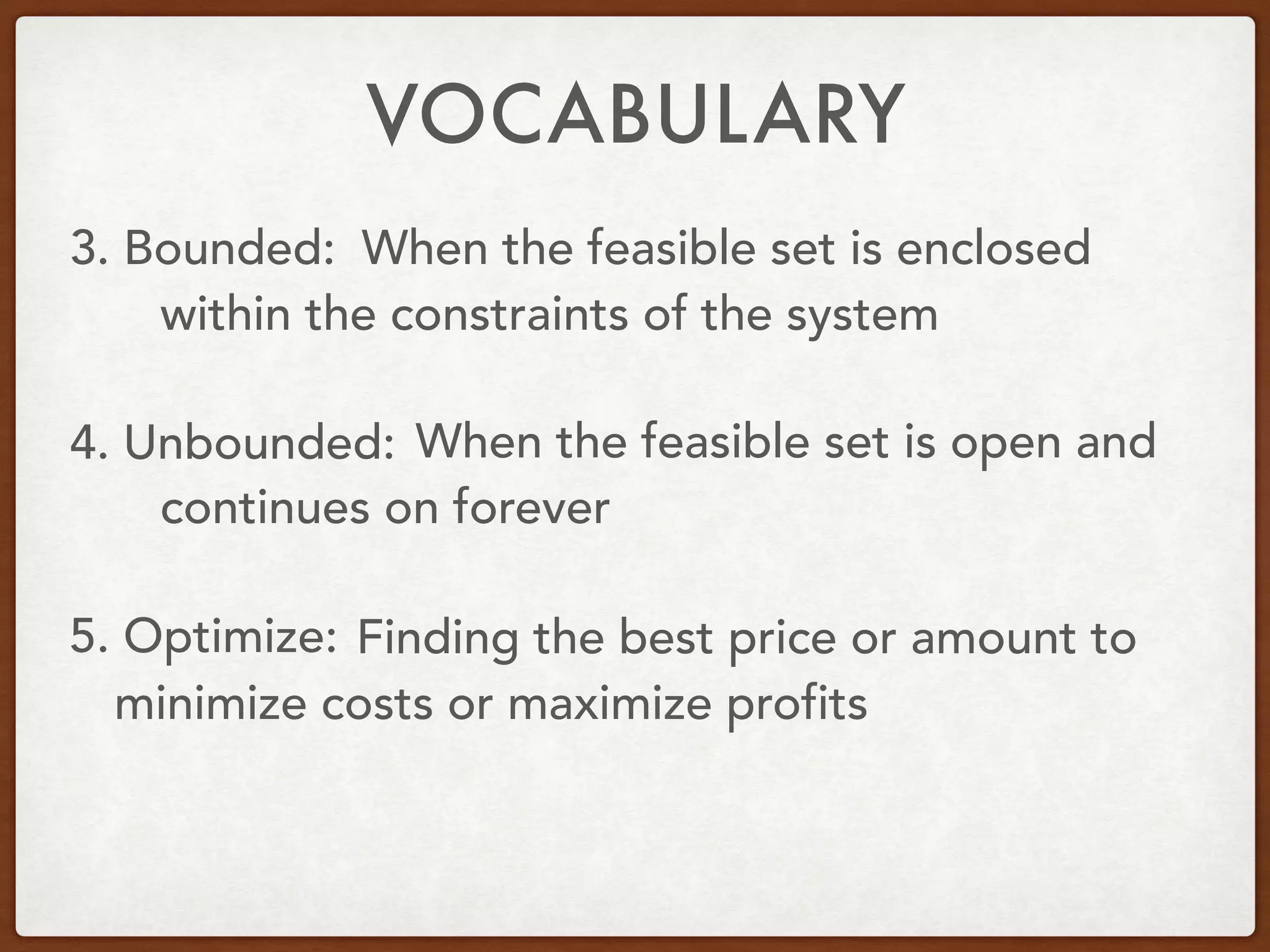
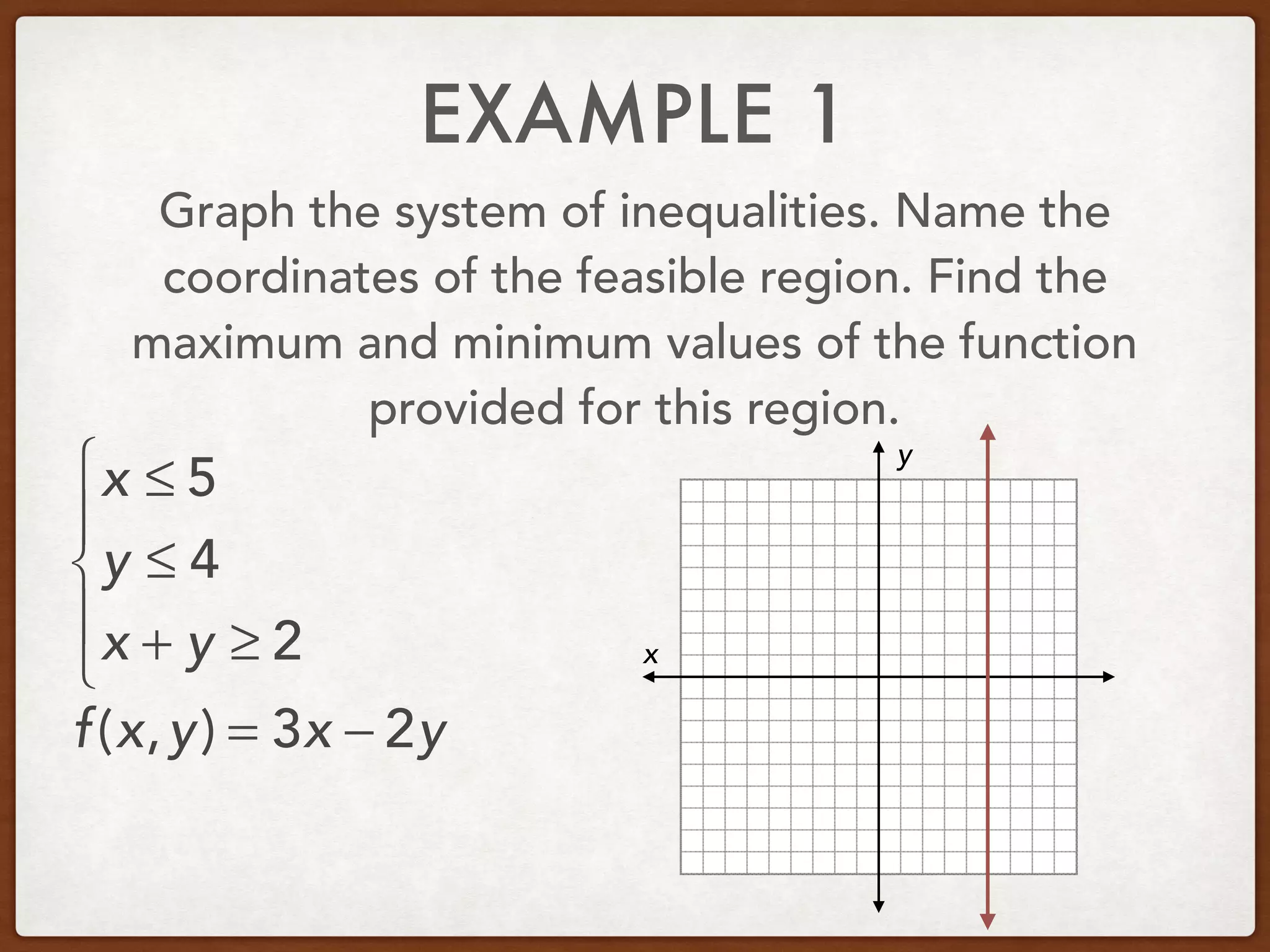
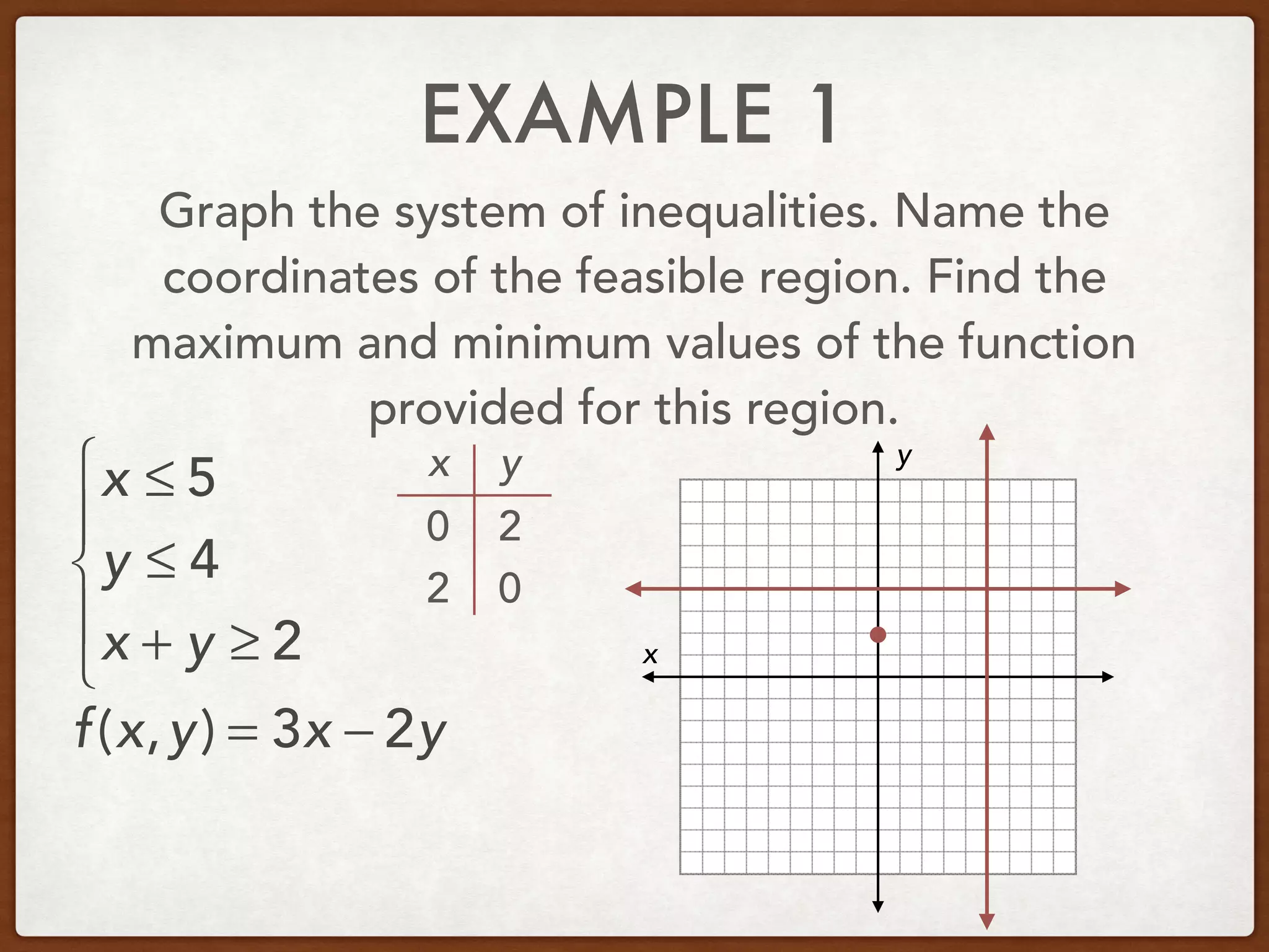
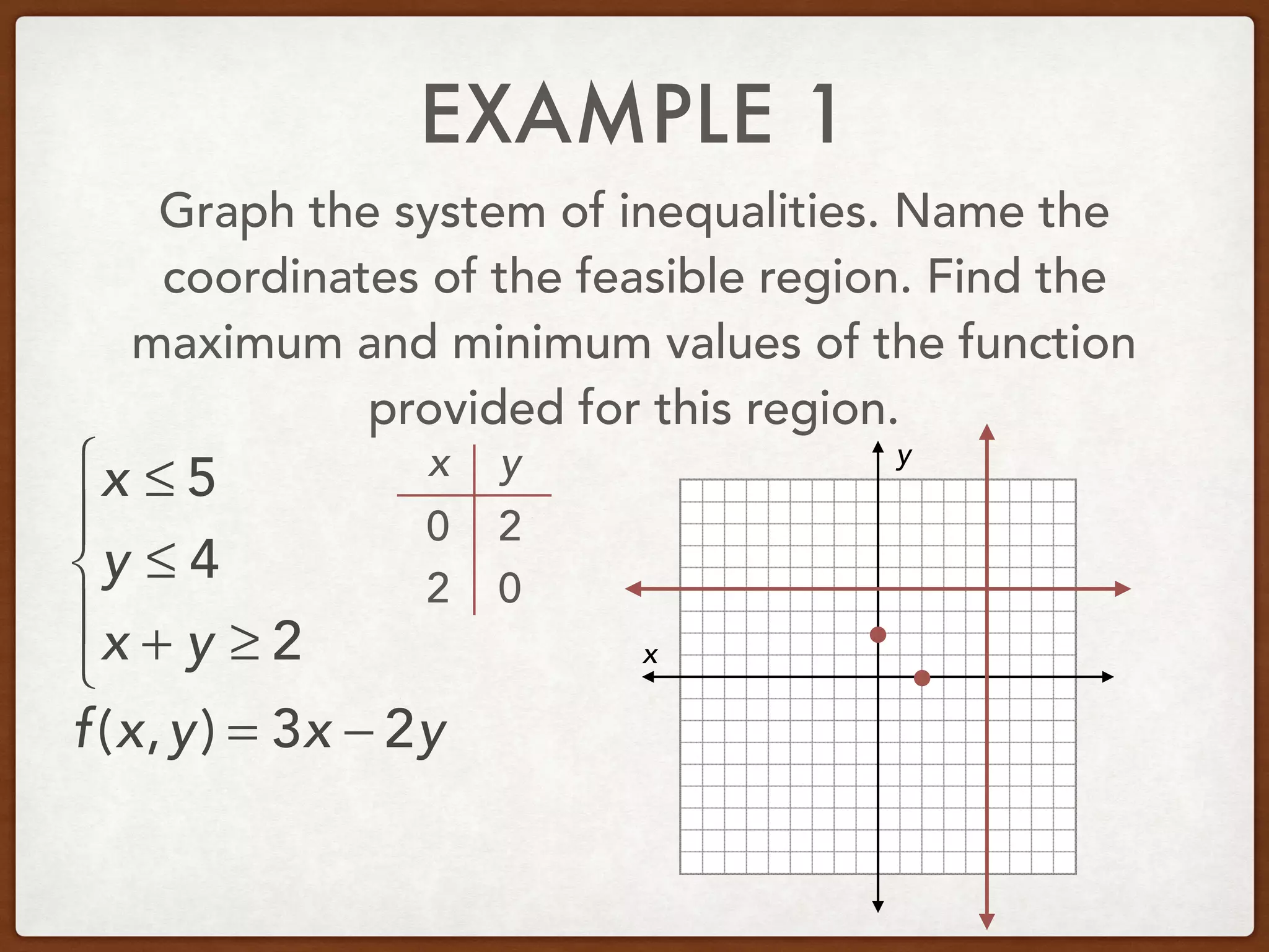
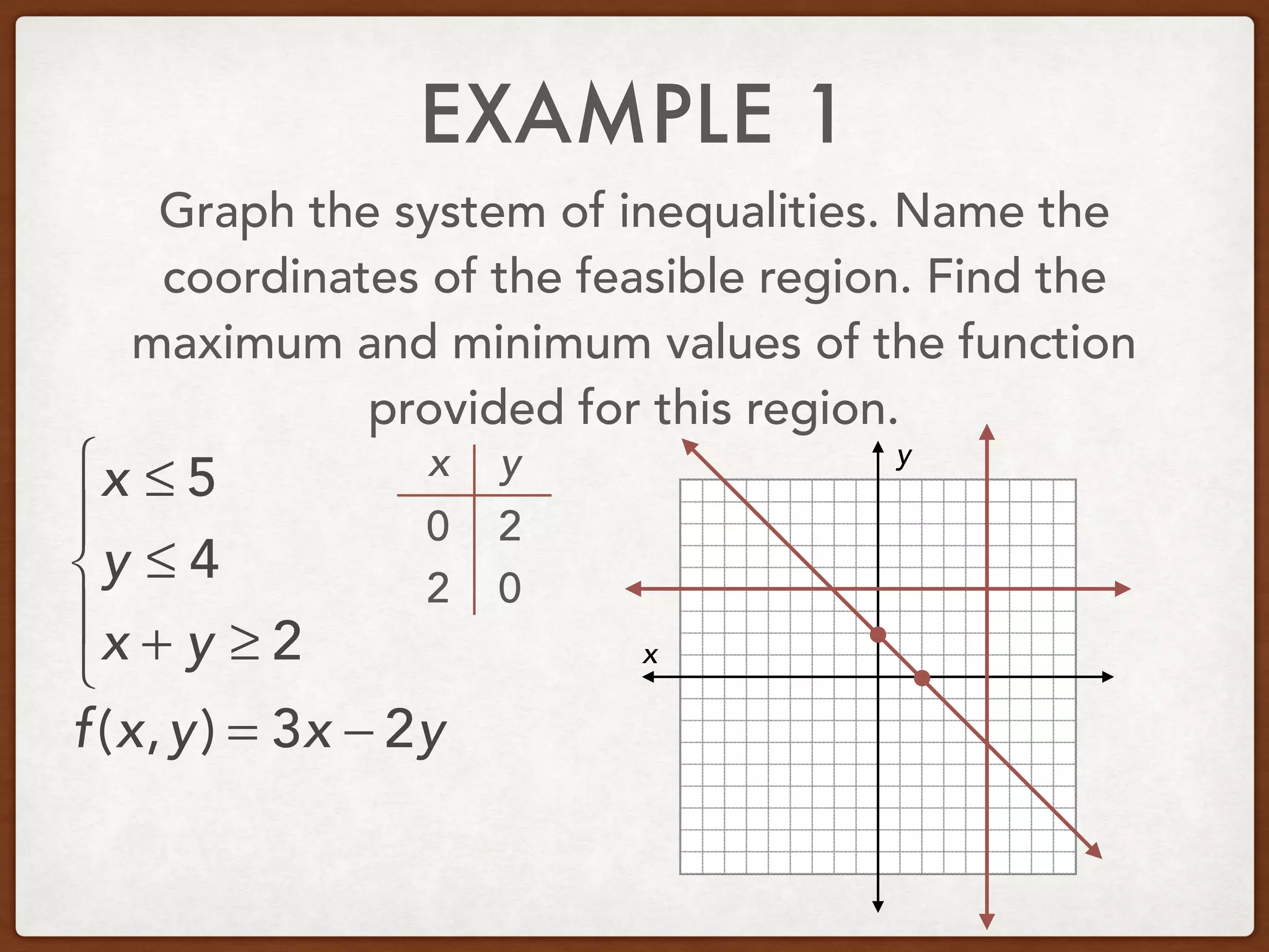
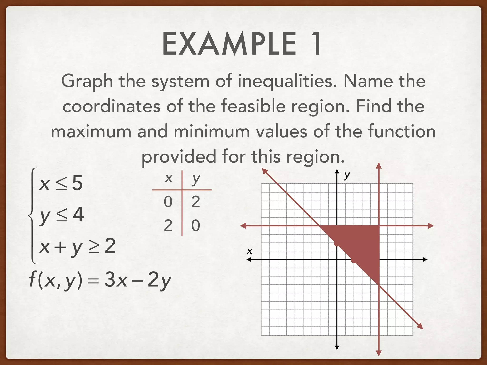
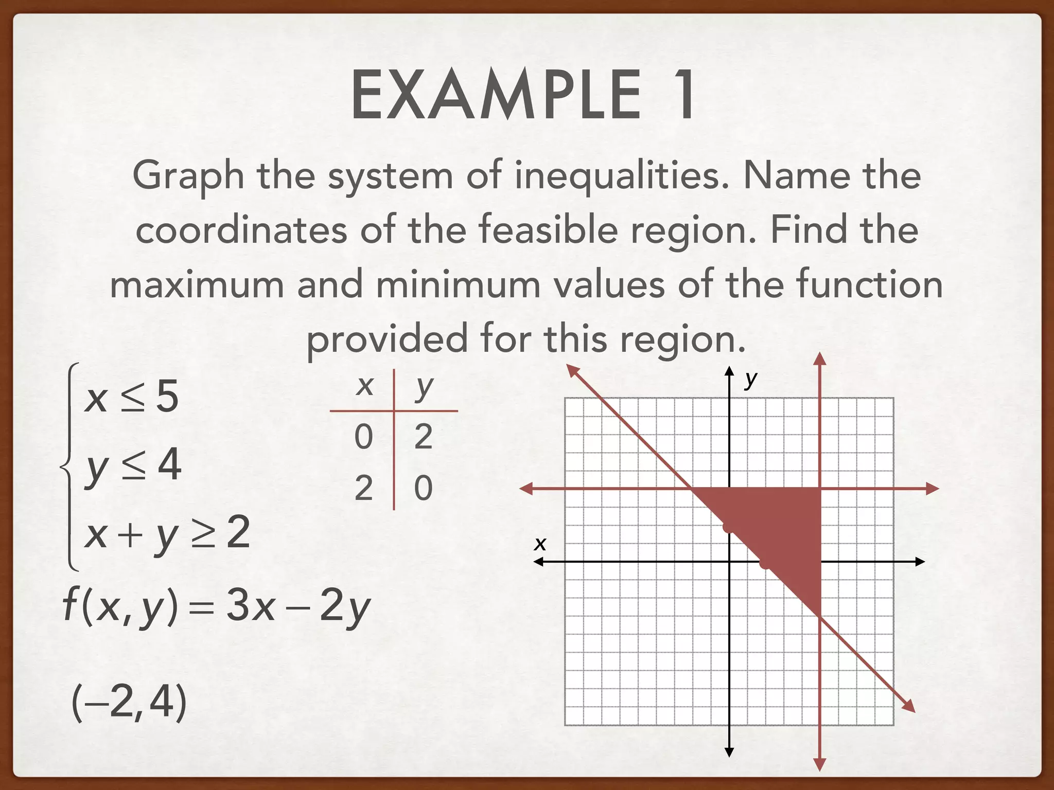
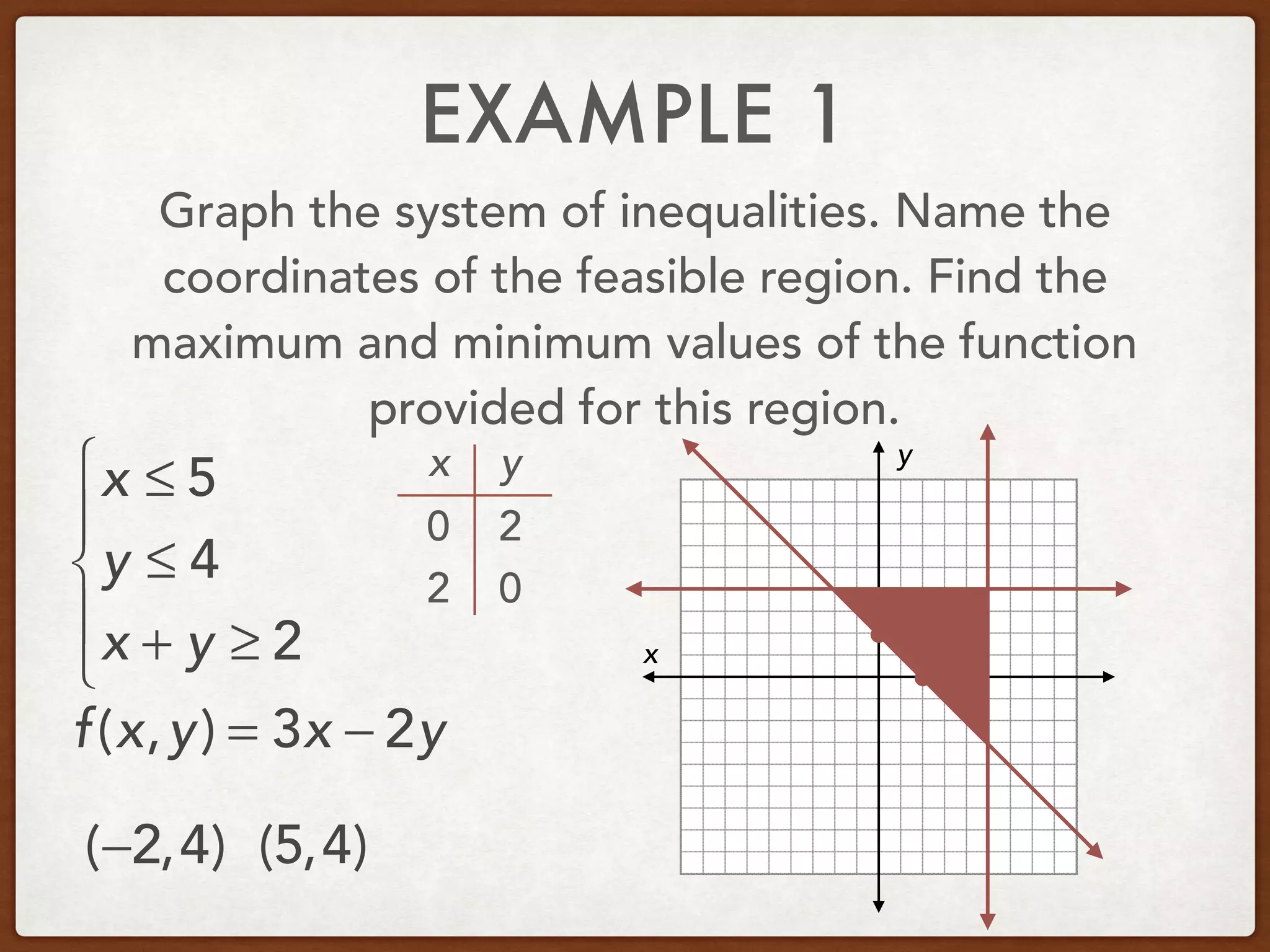
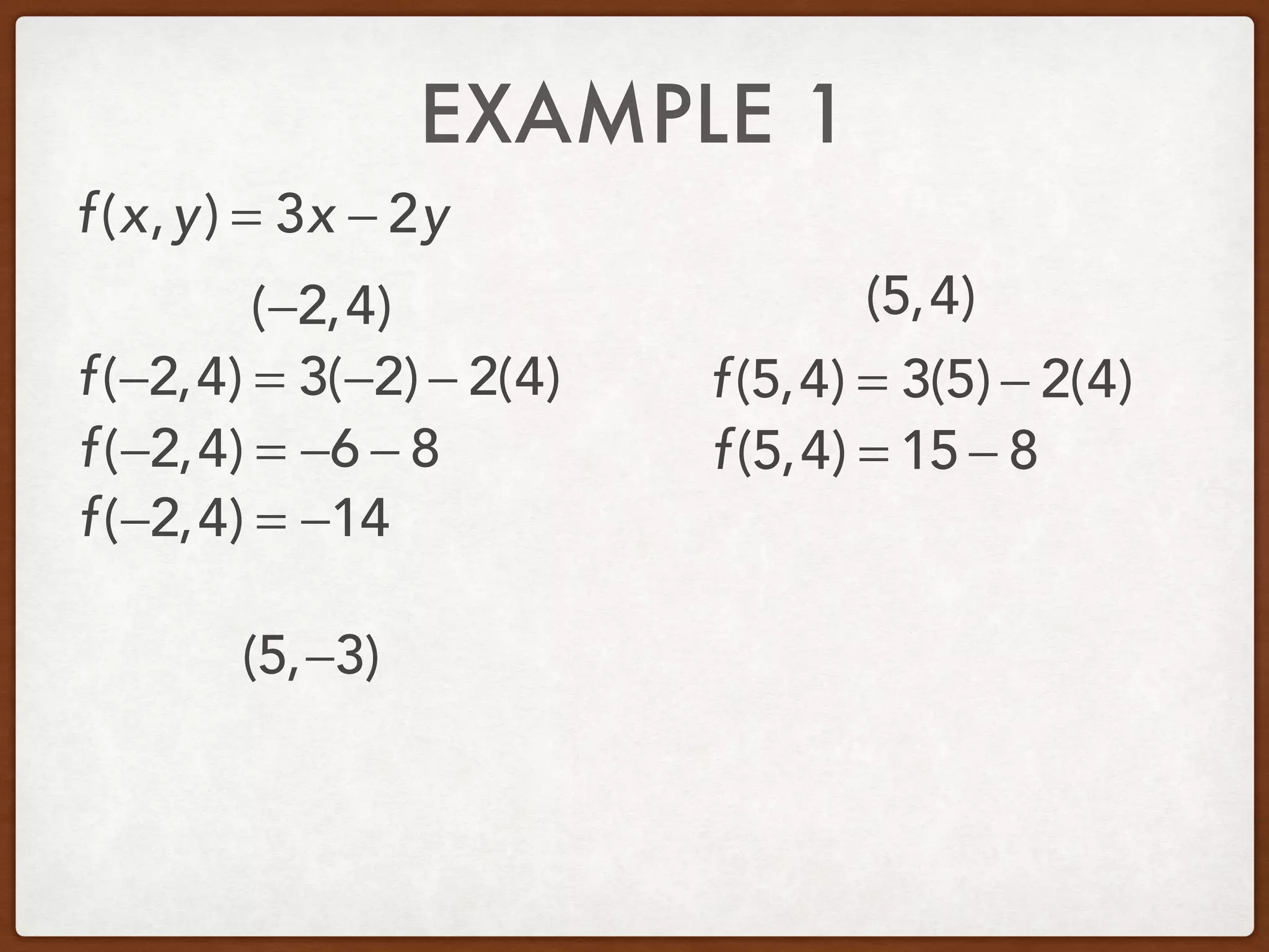
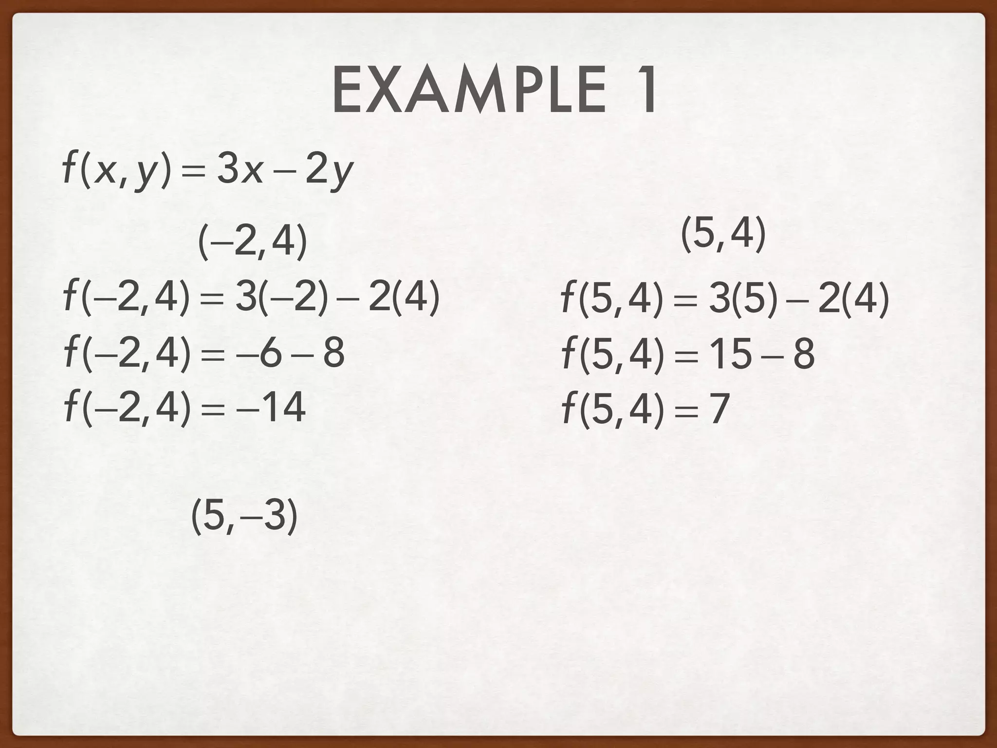
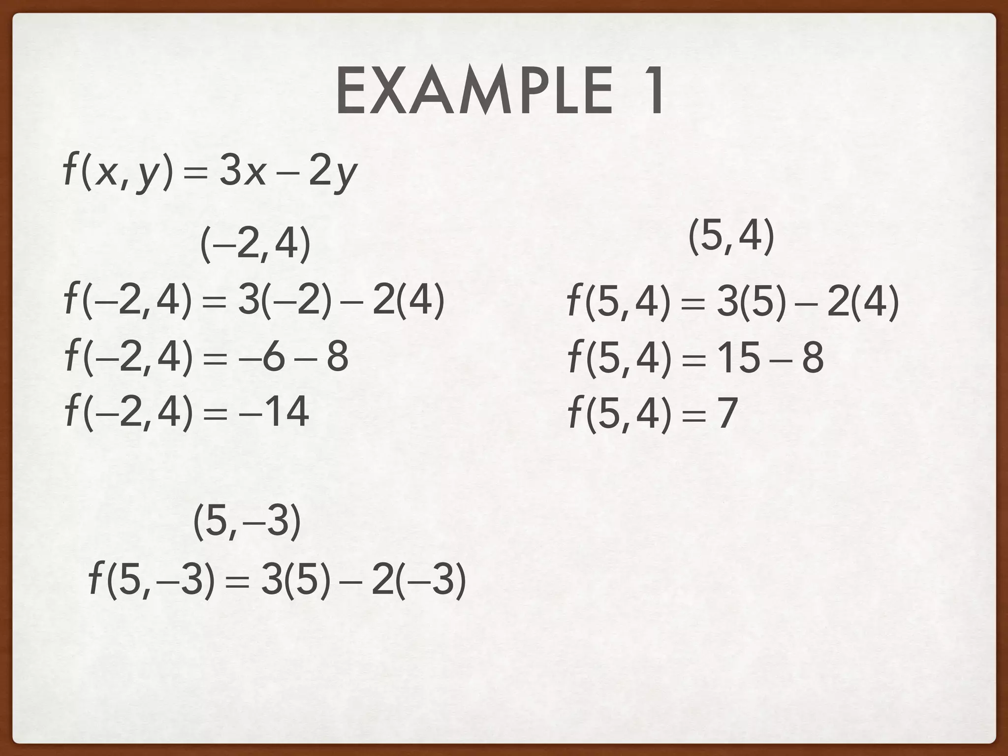
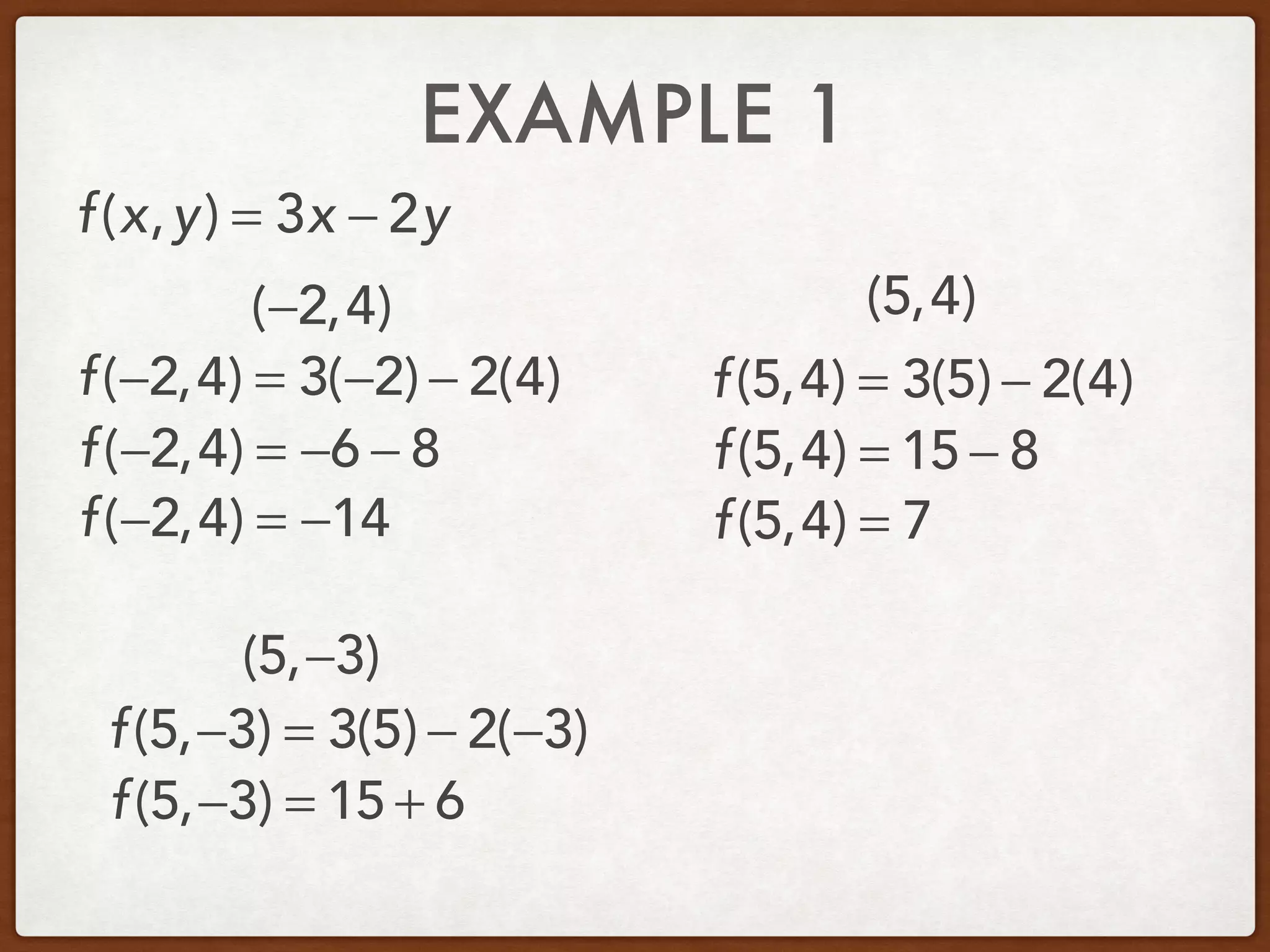
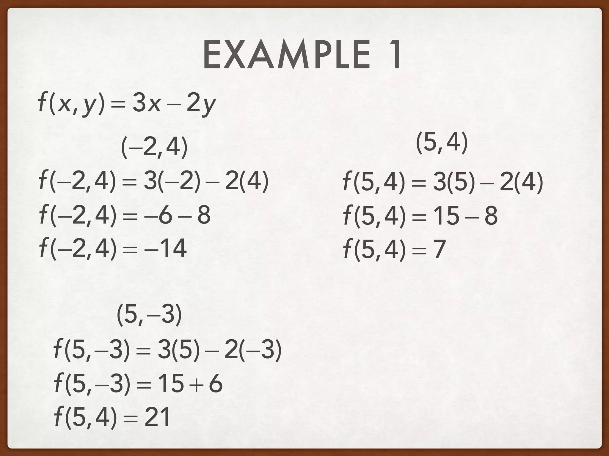
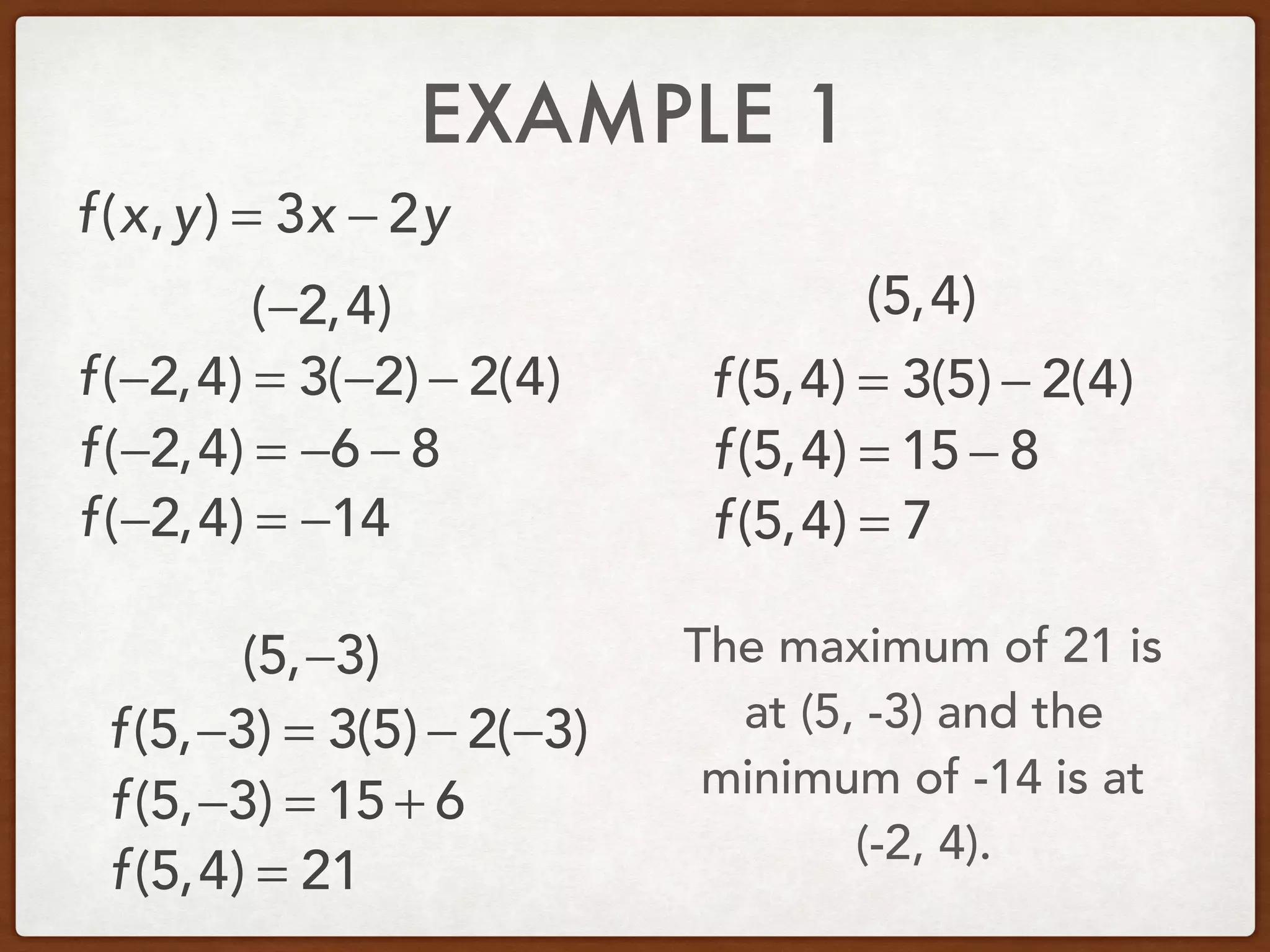
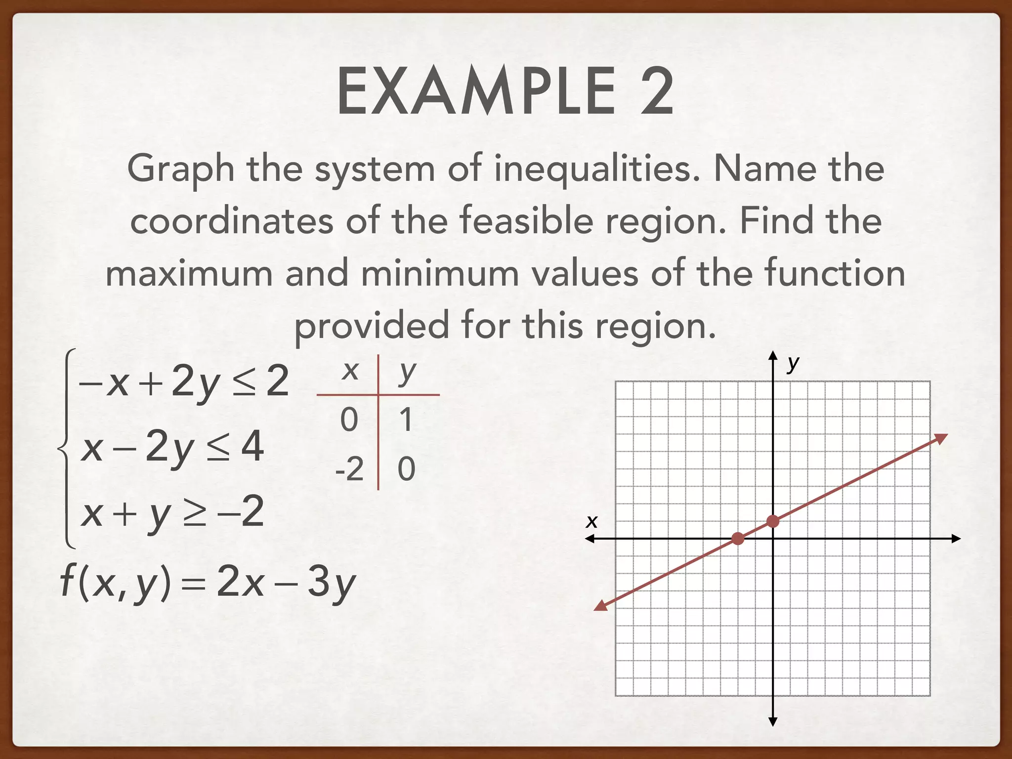
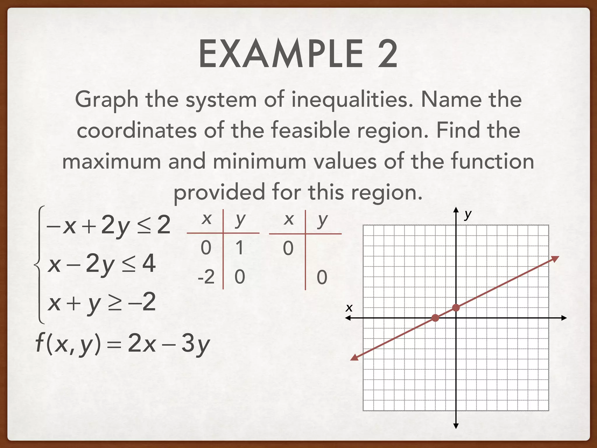
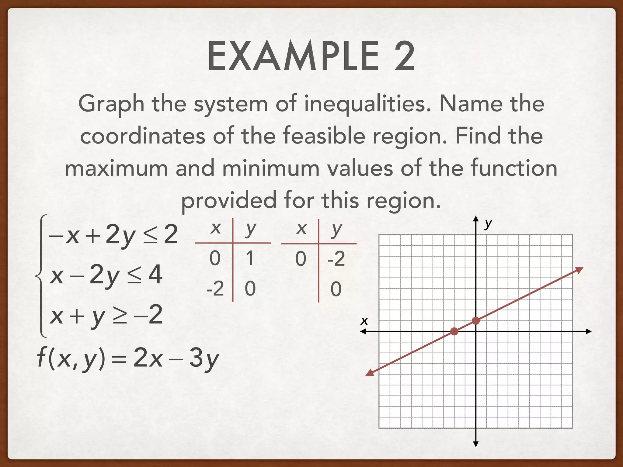
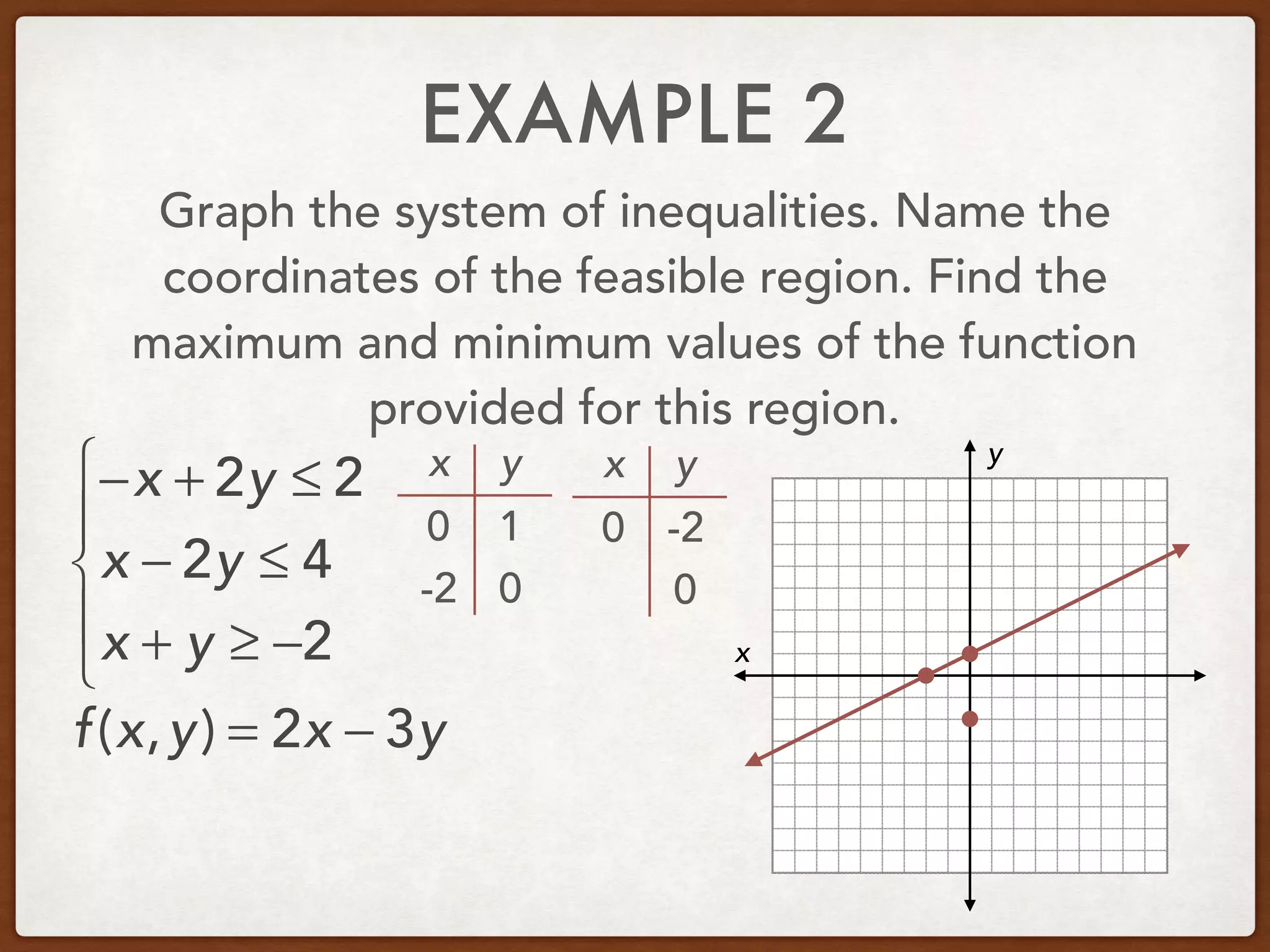
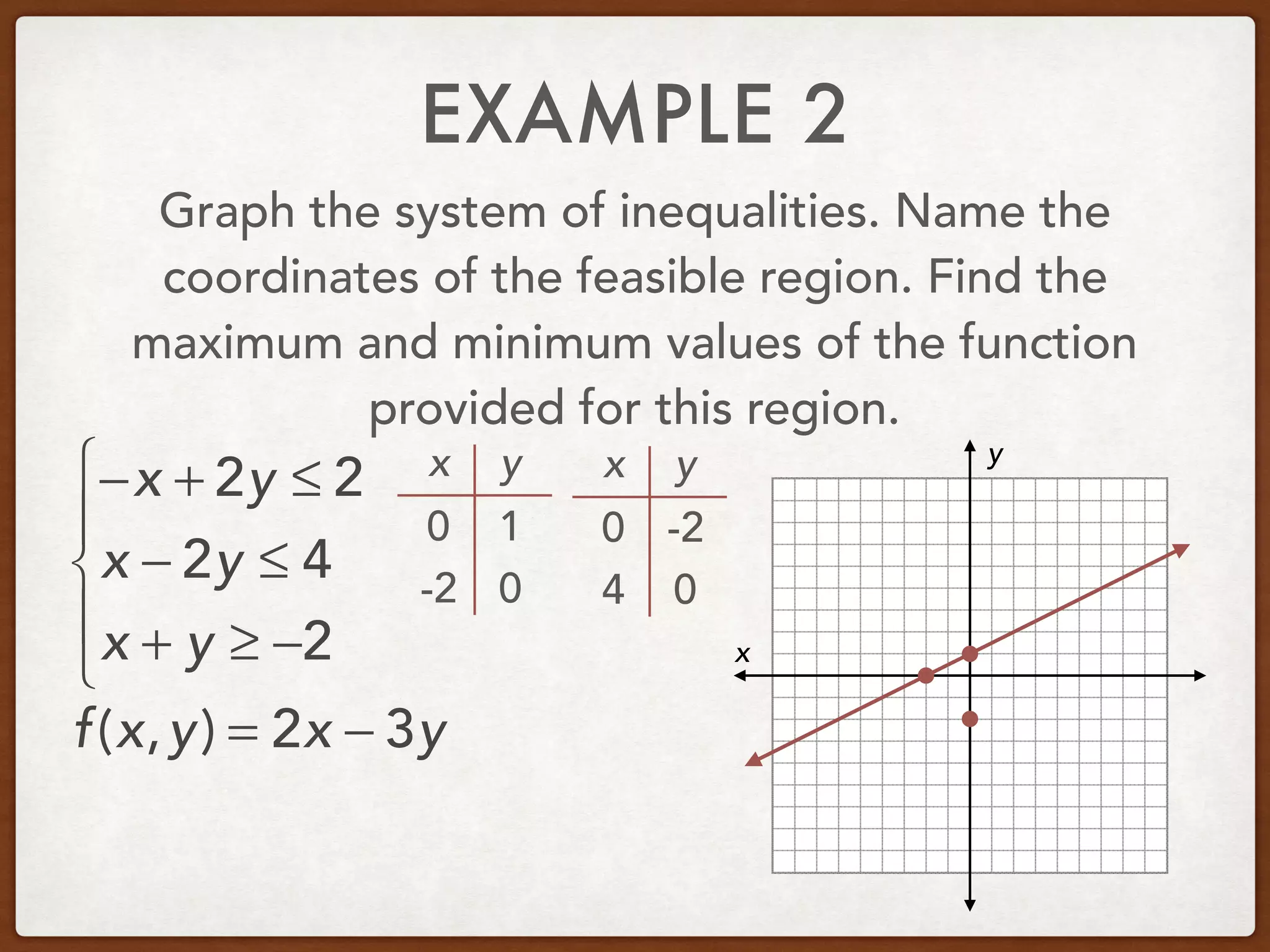
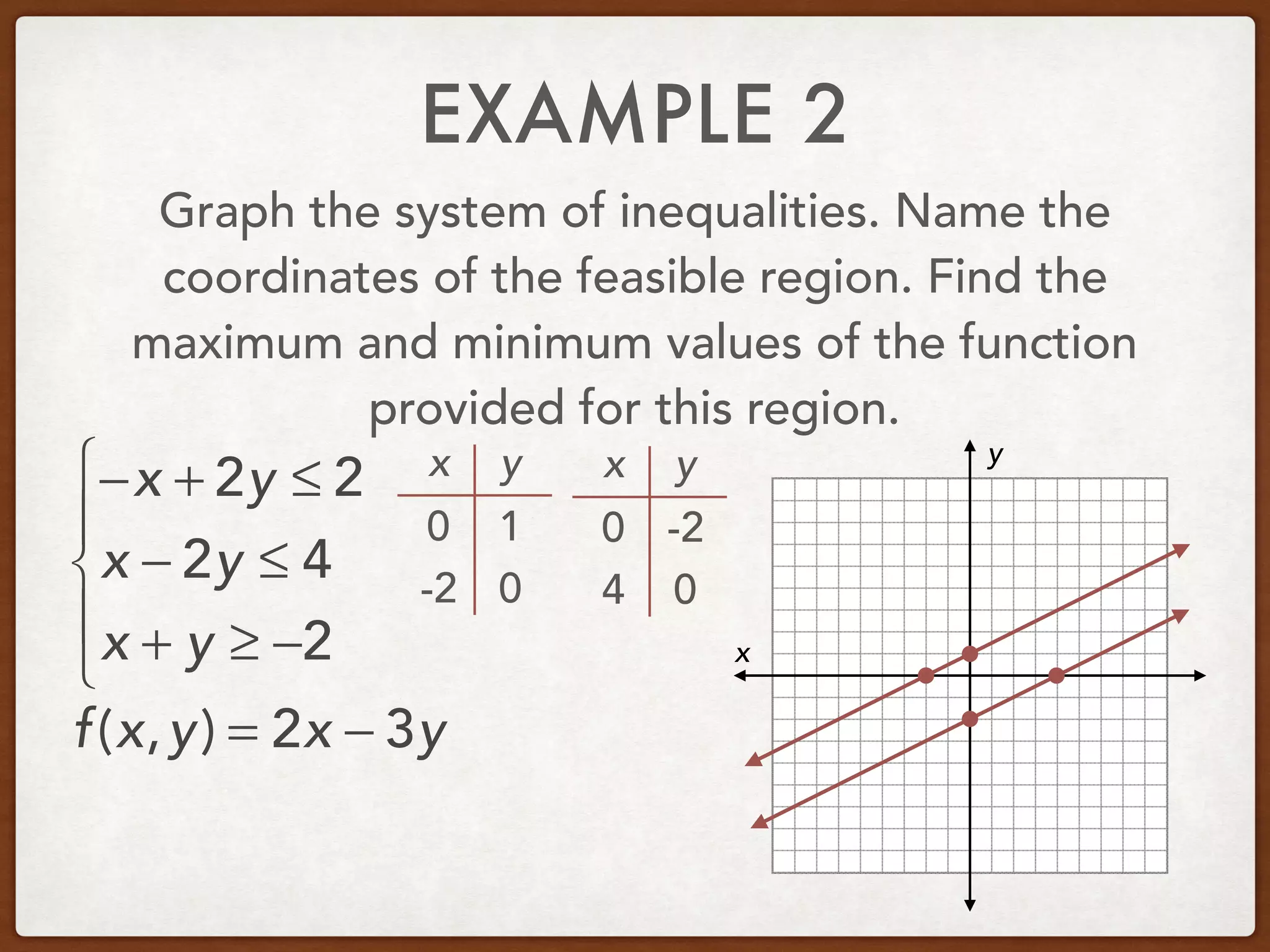
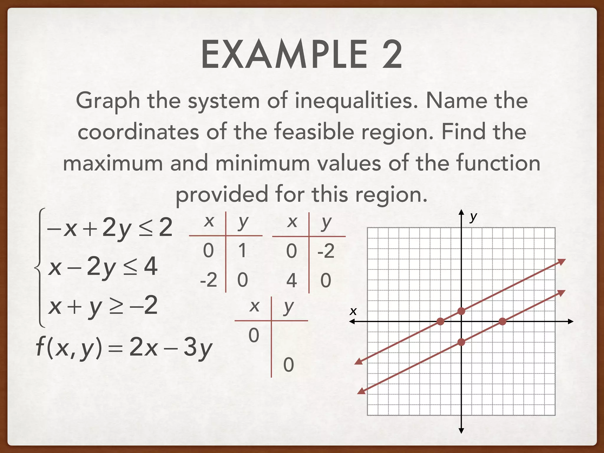
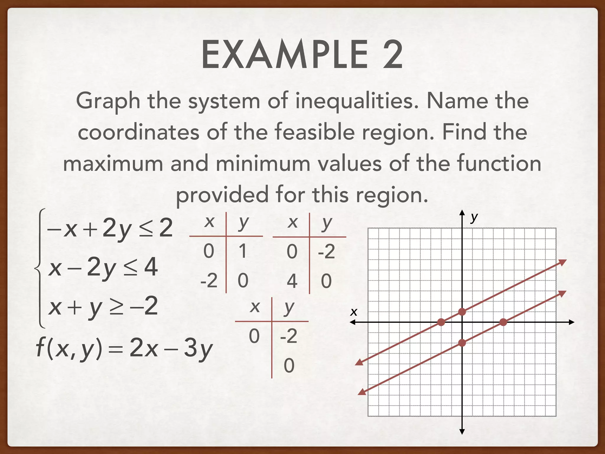
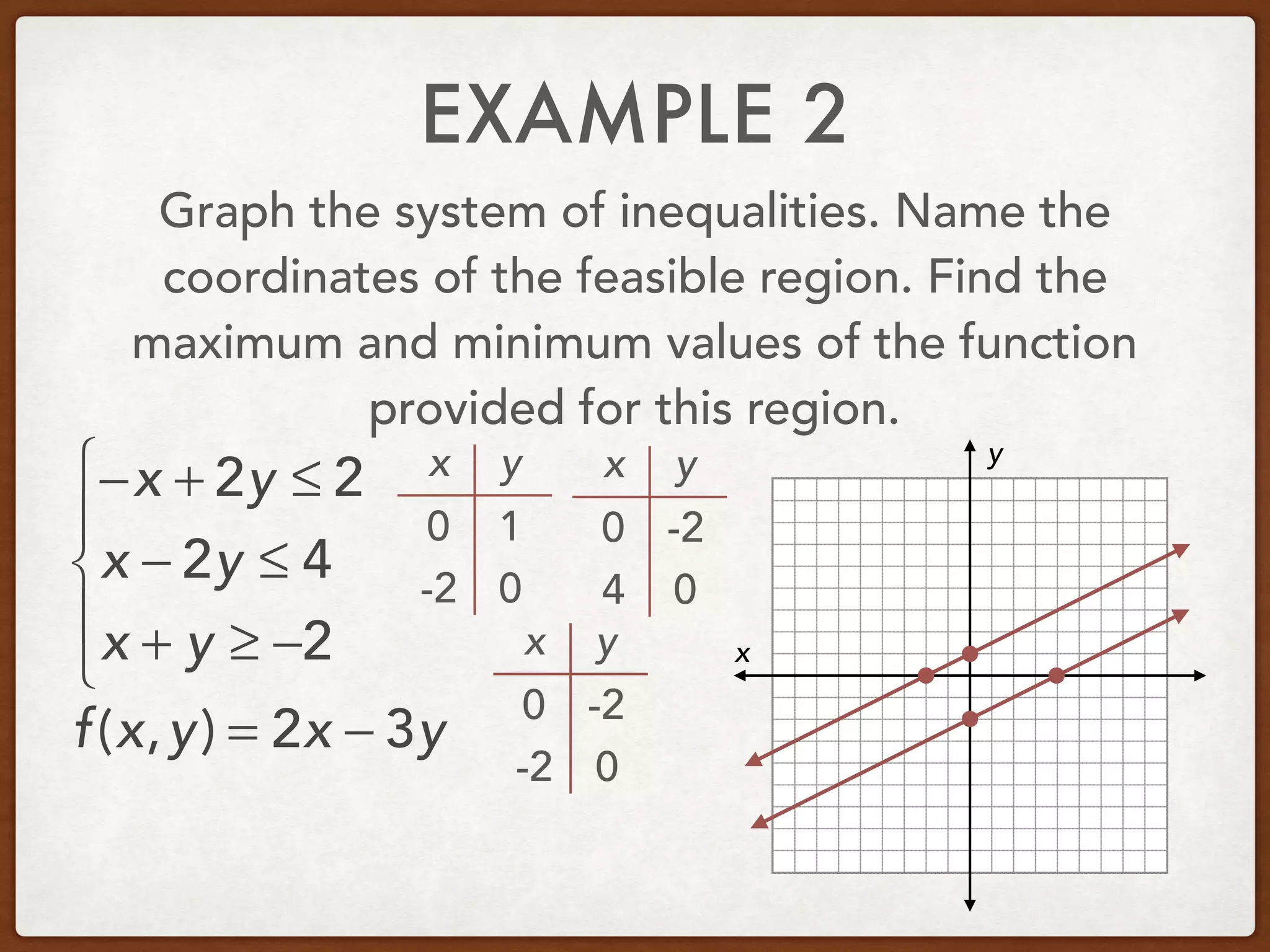
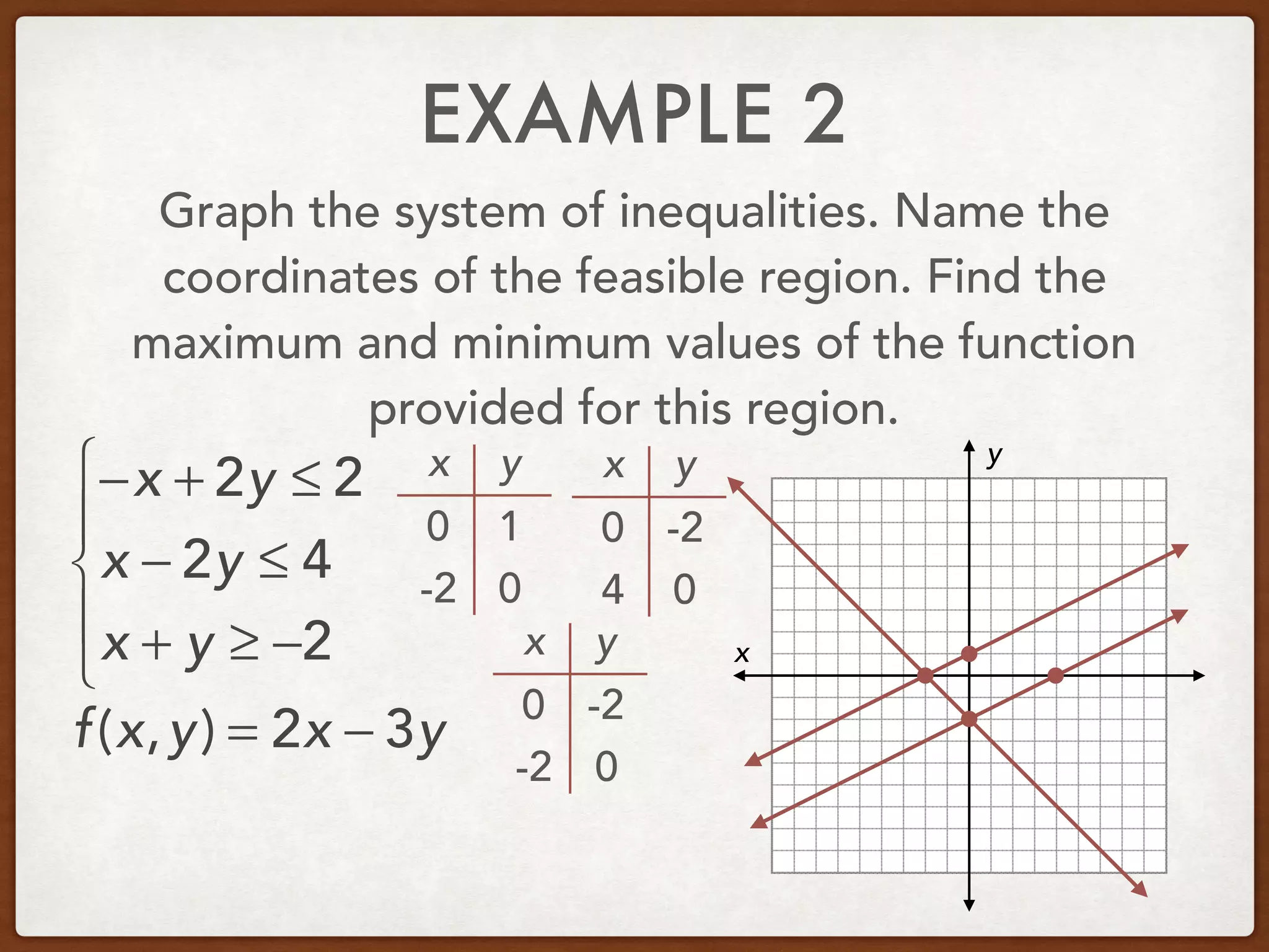
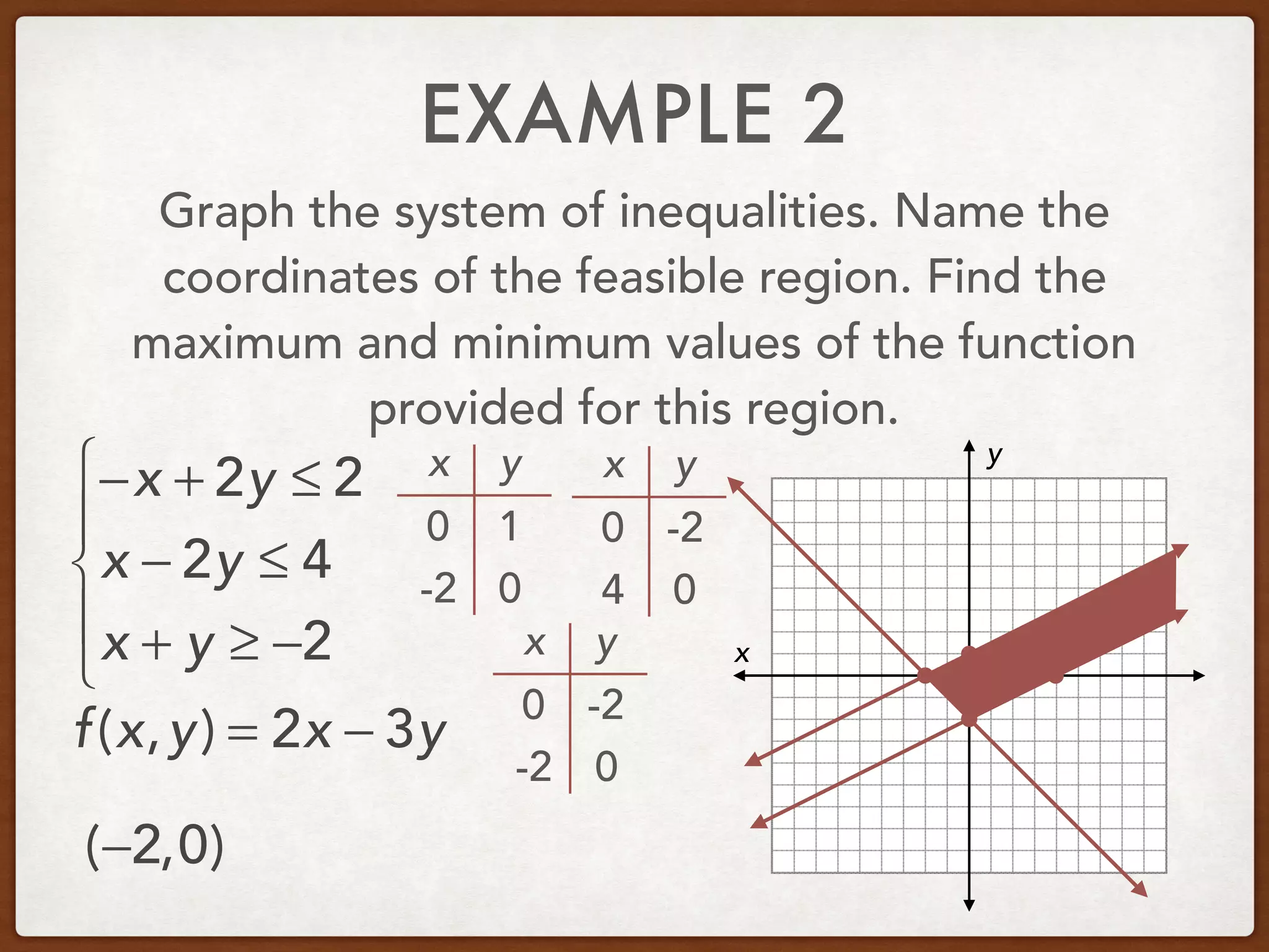
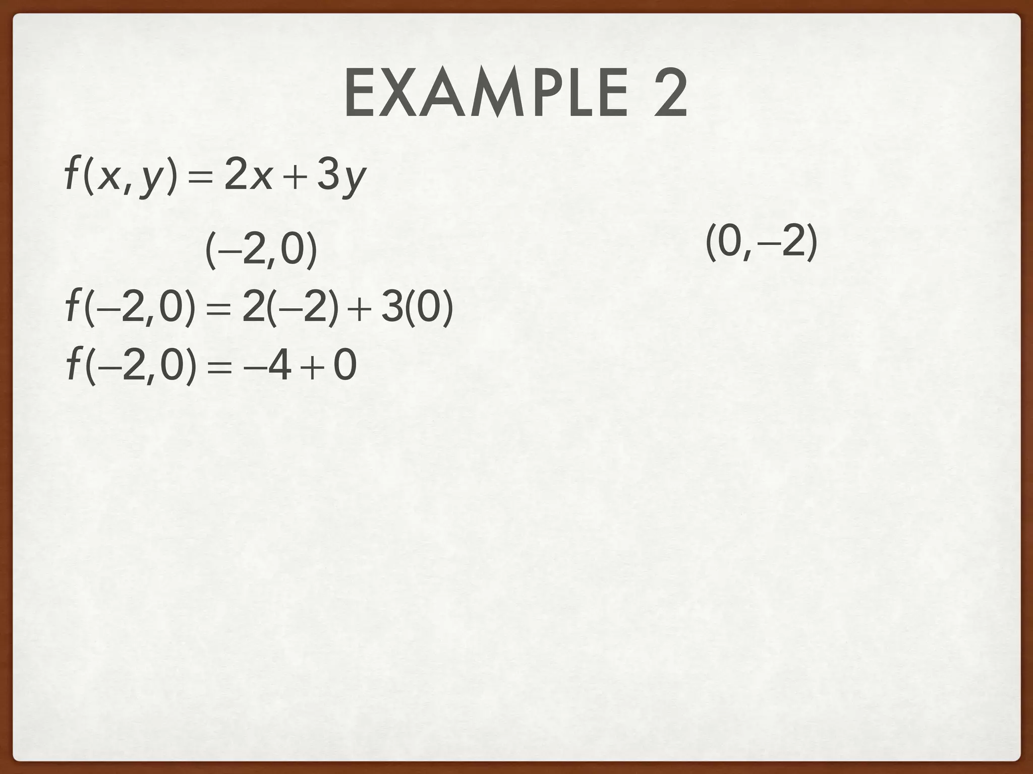
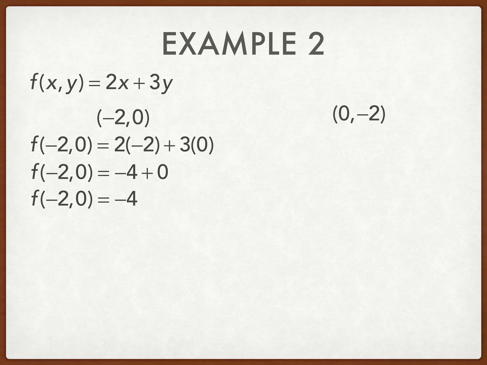
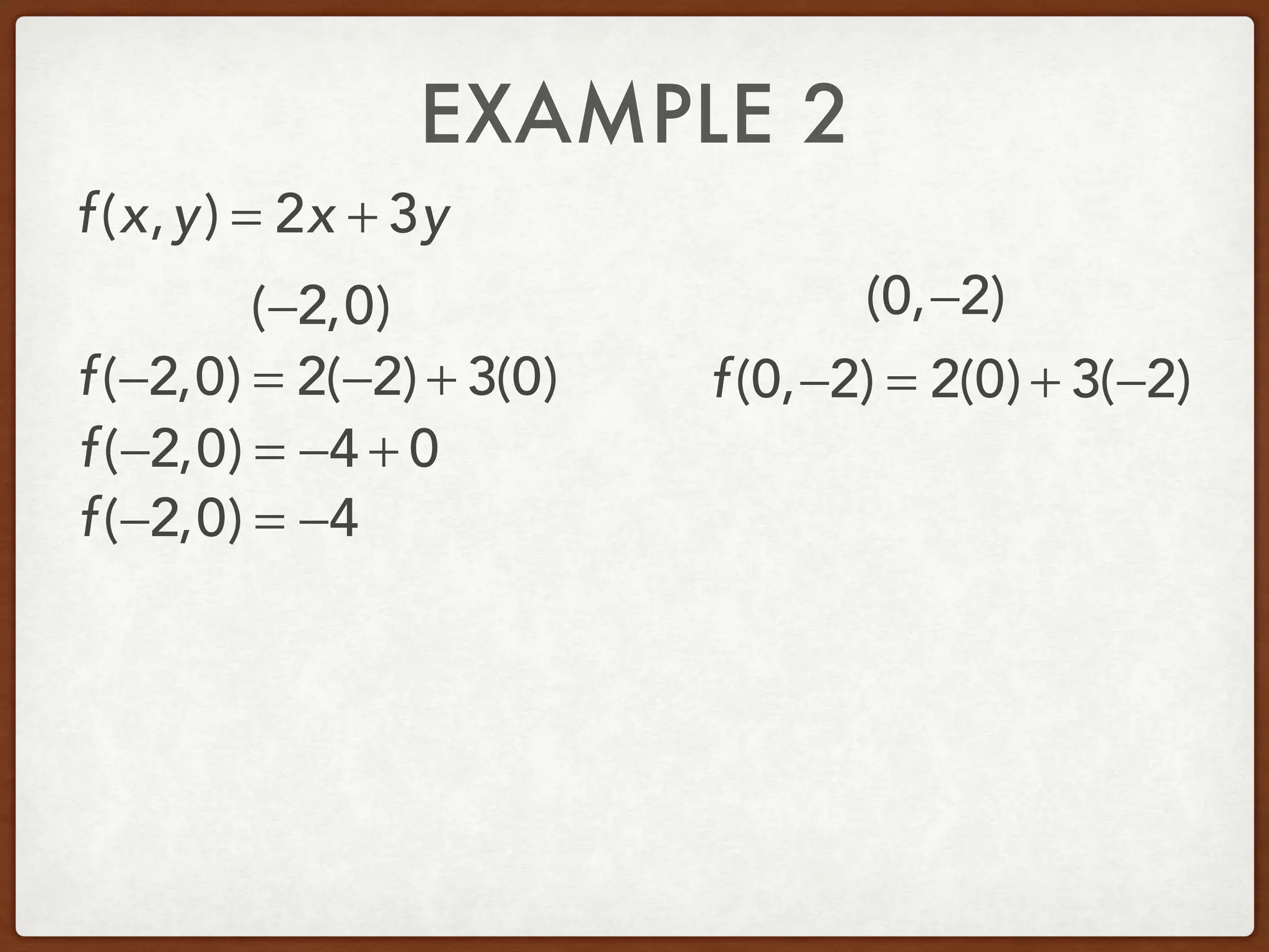
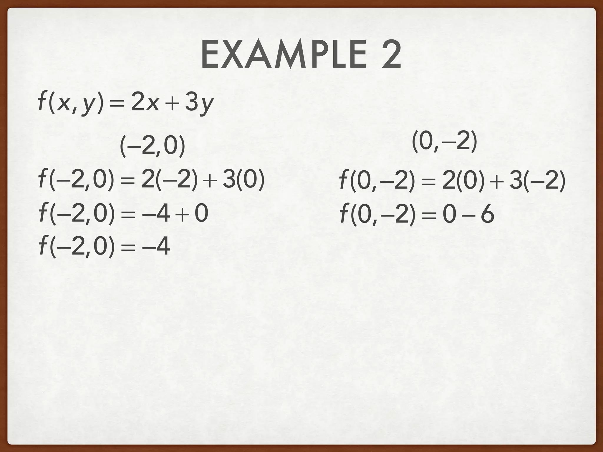
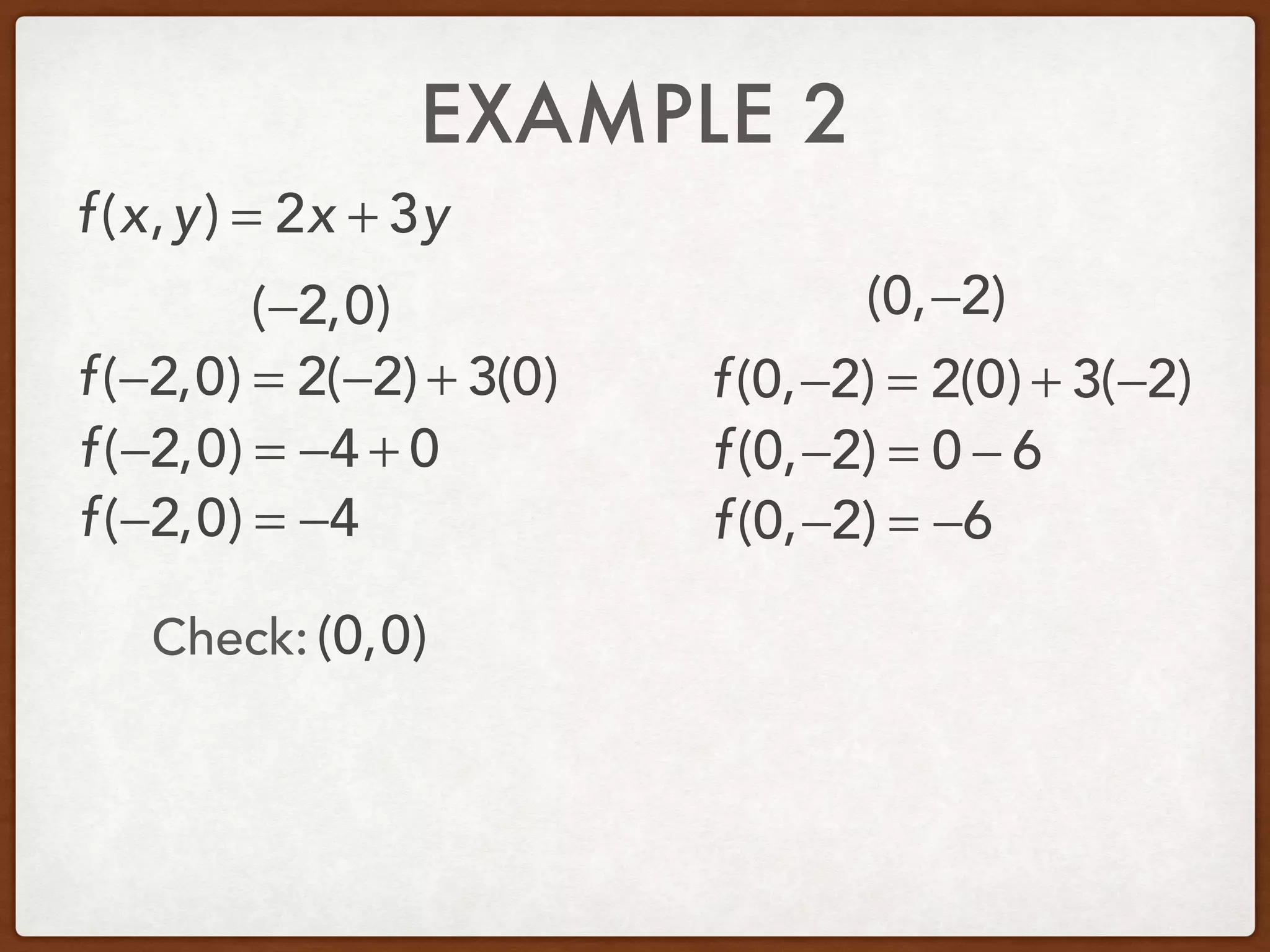
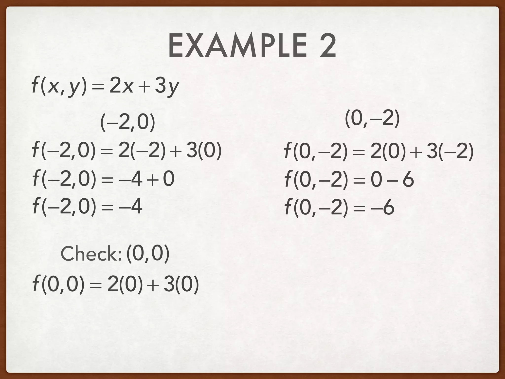
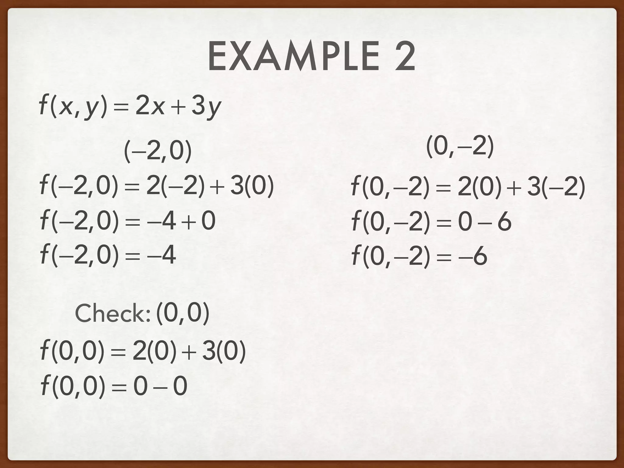
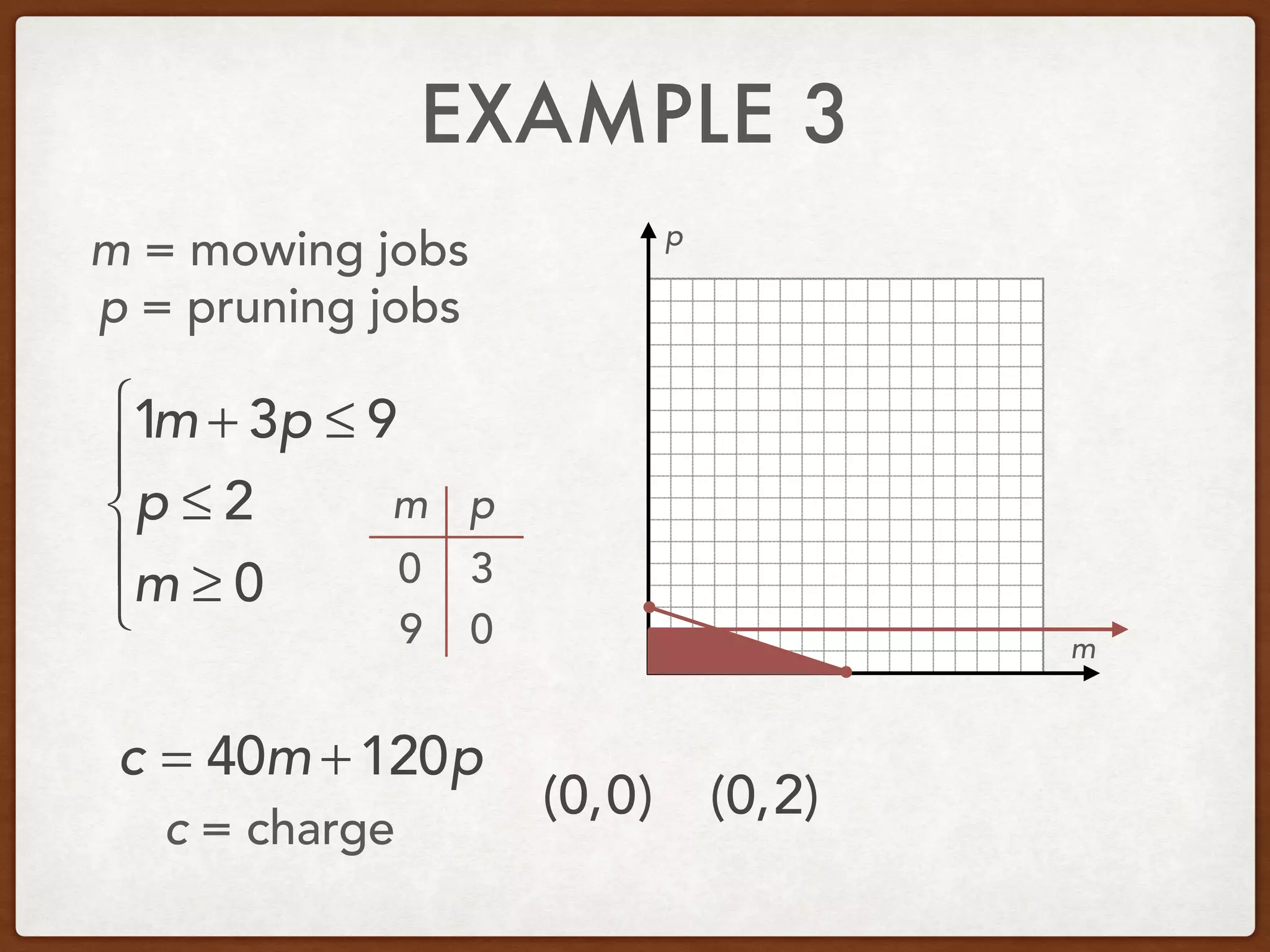
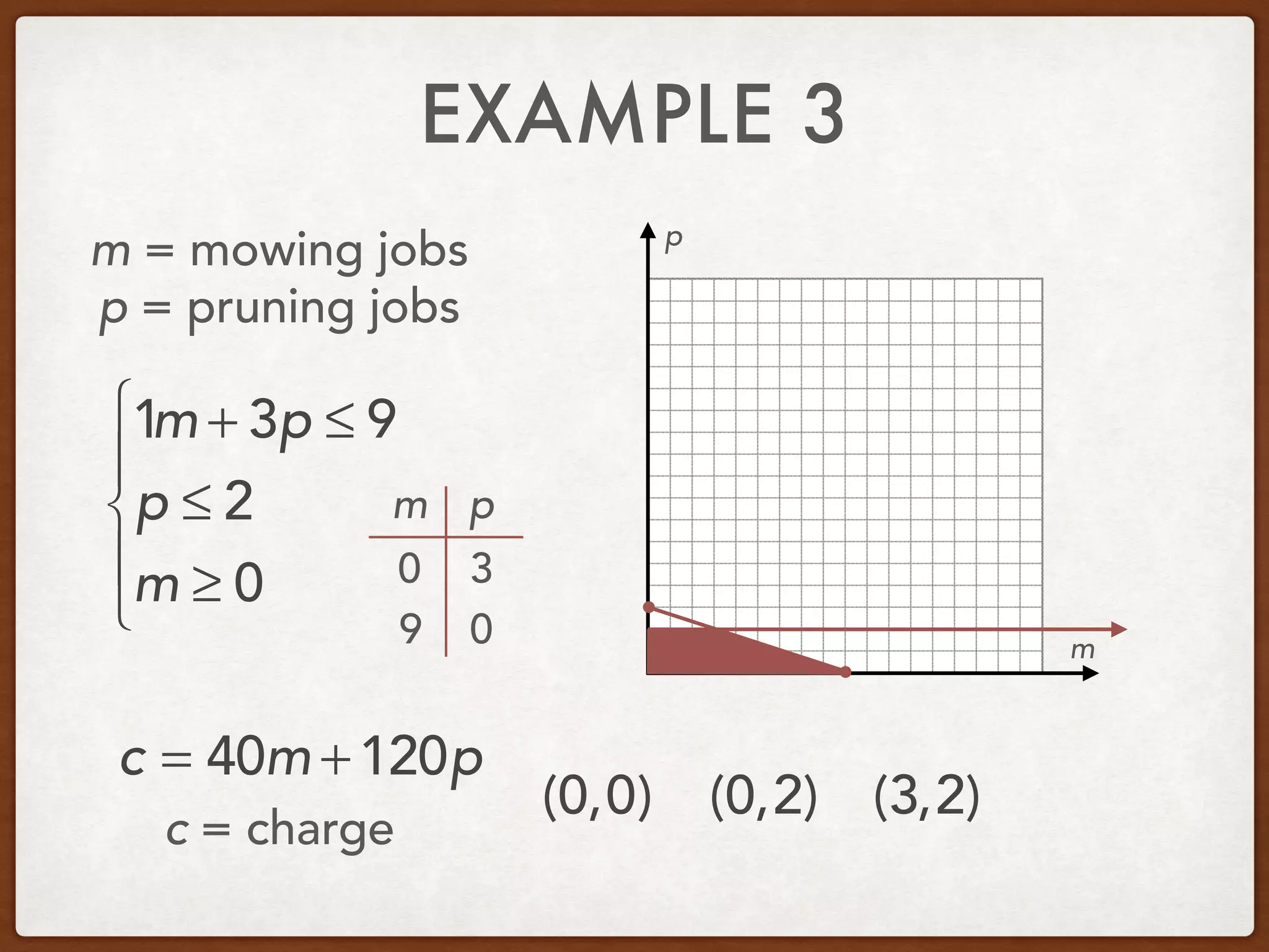
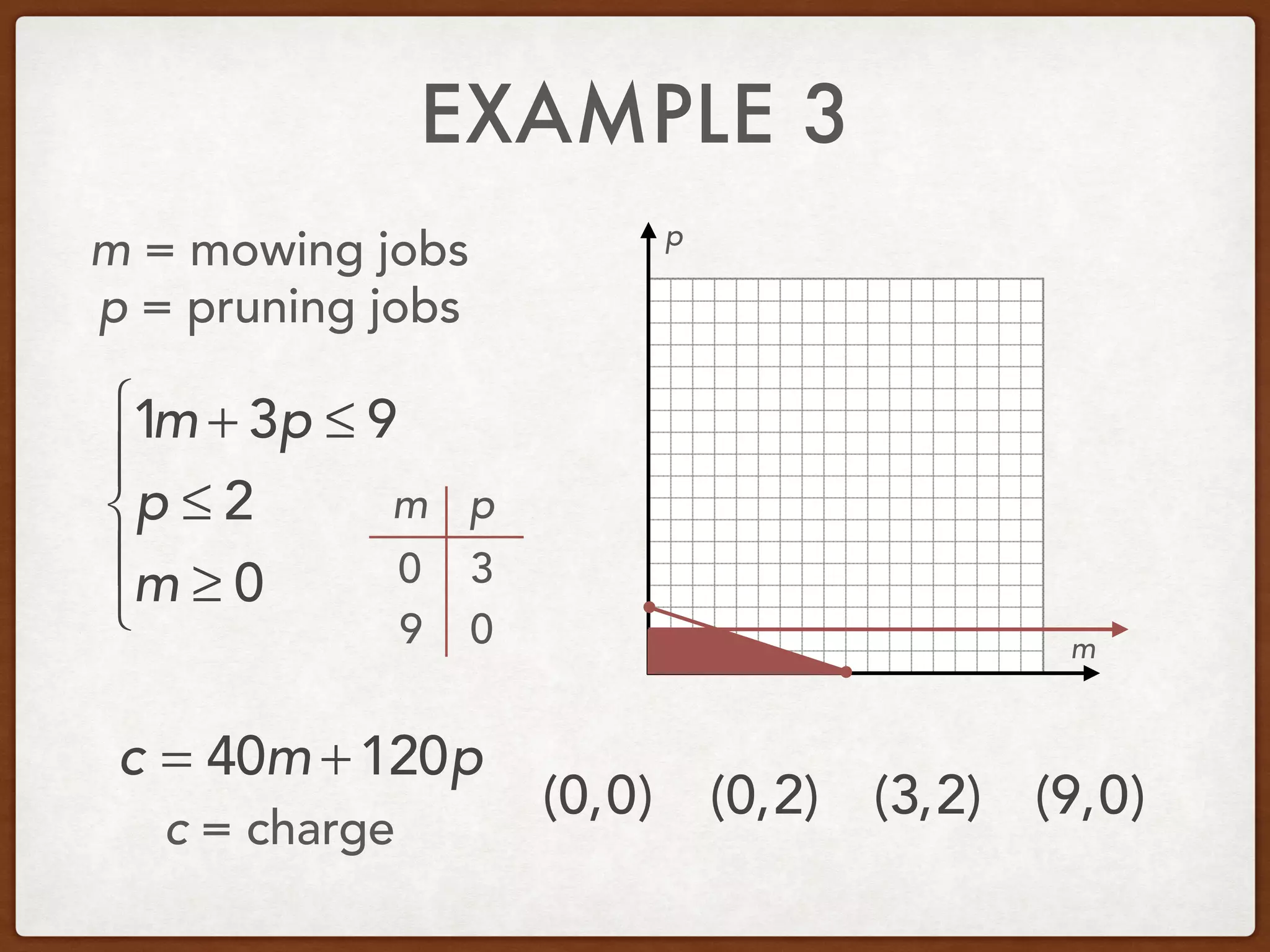
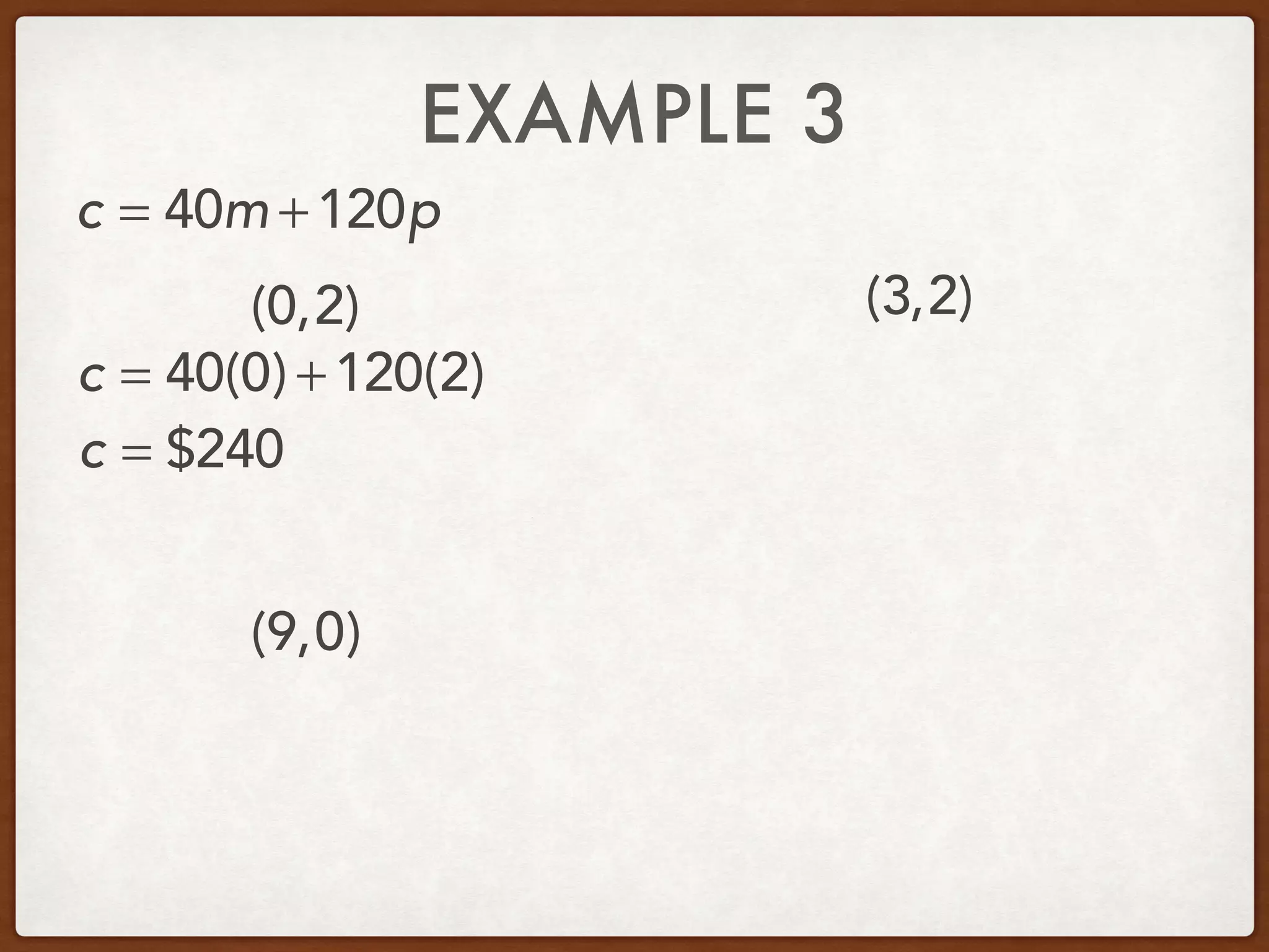
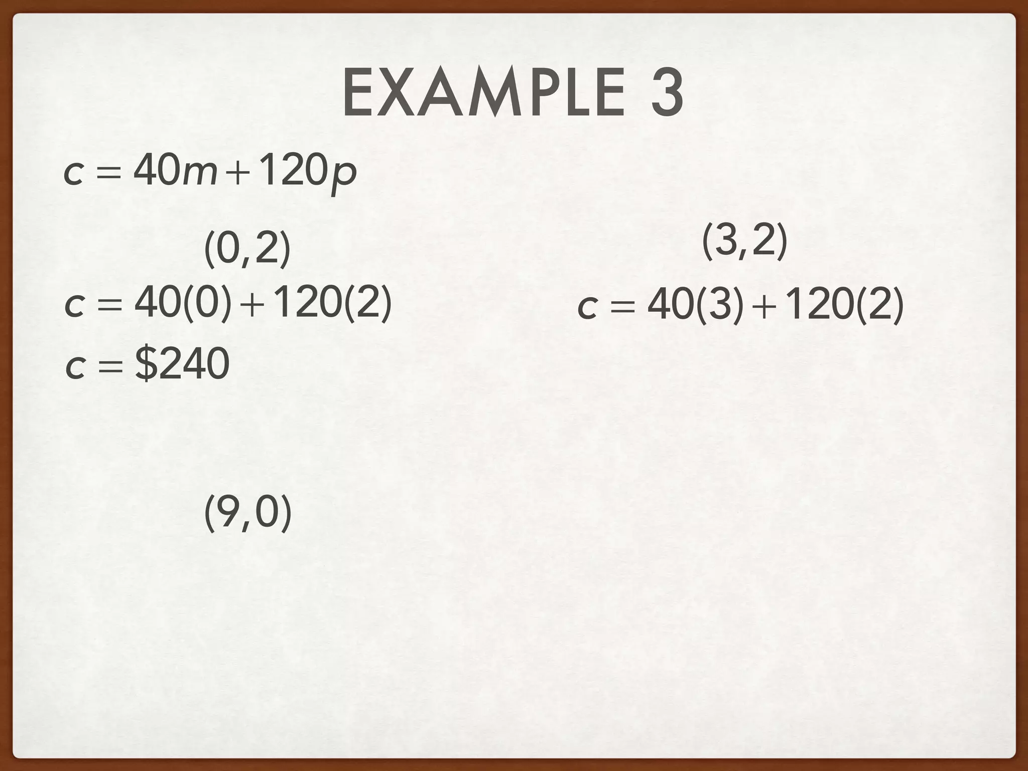
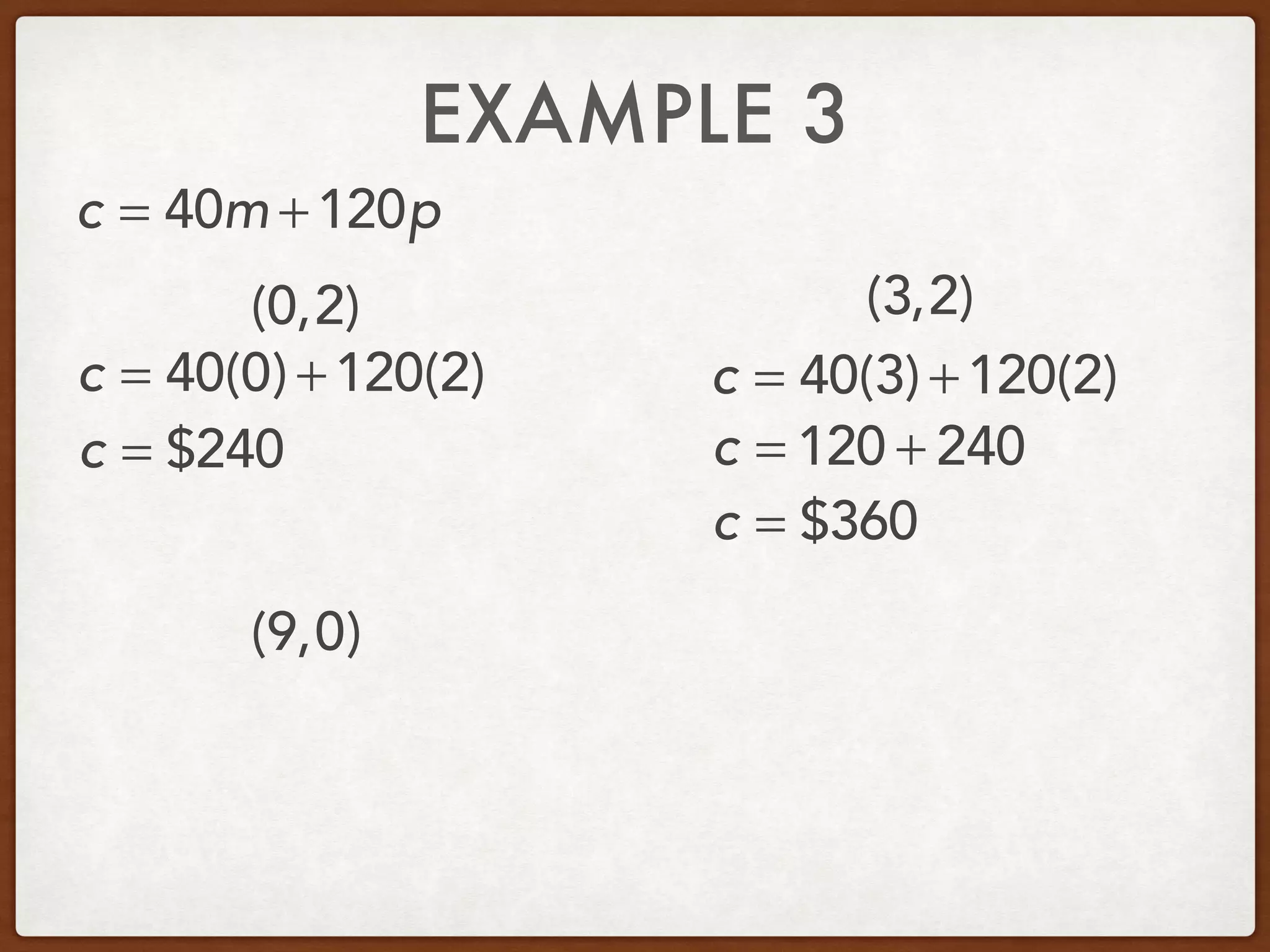
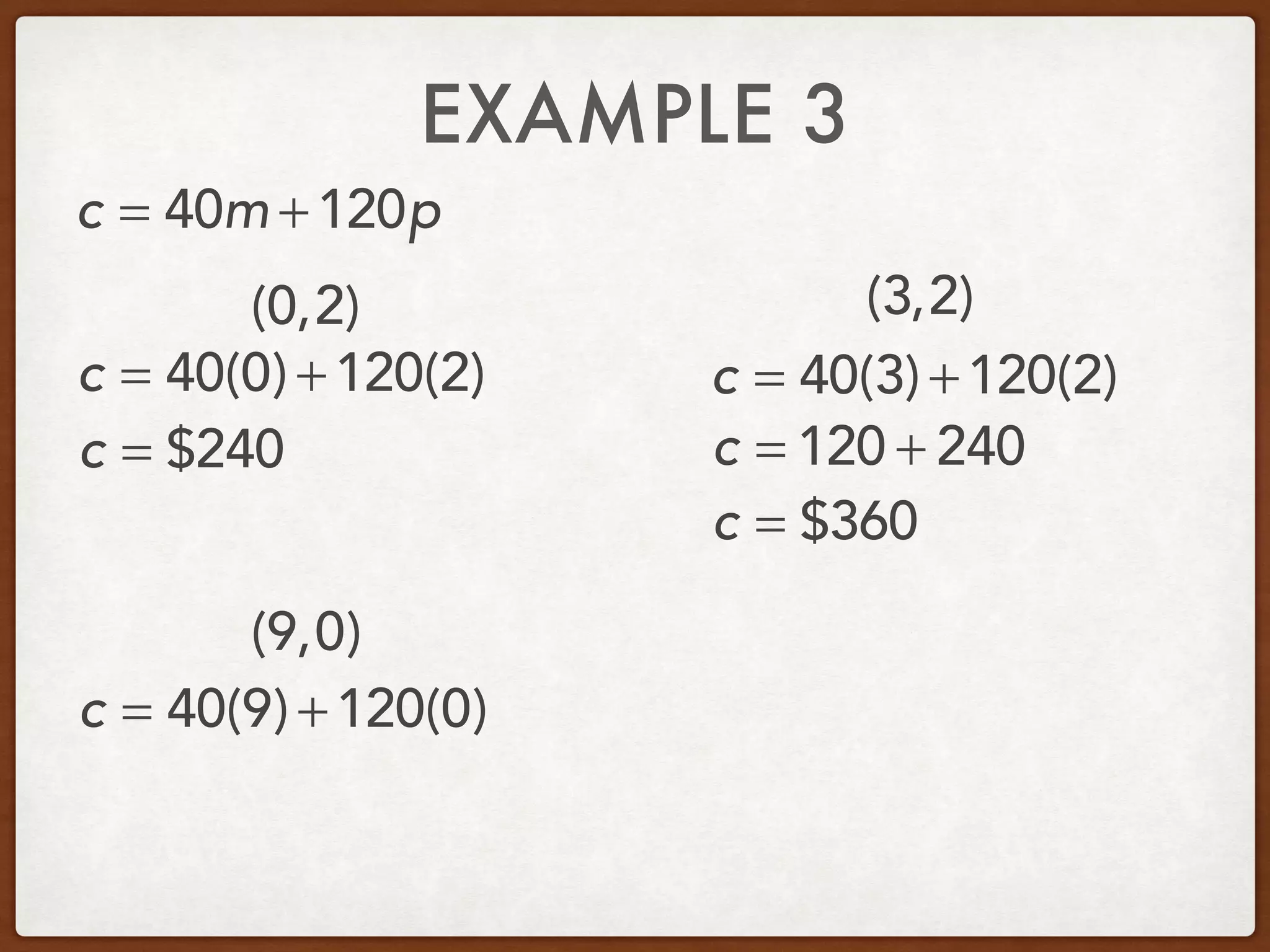
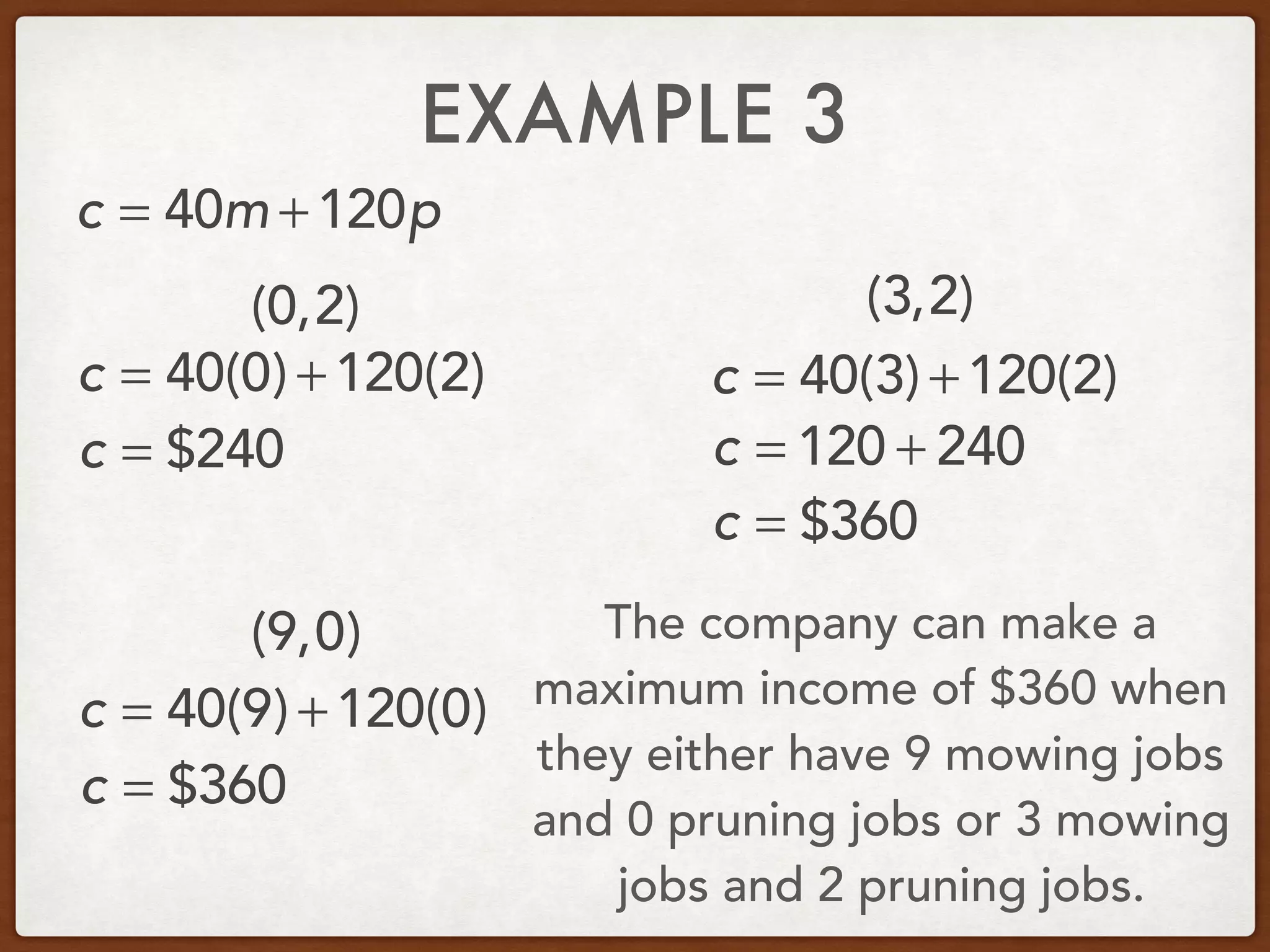
OPTIMIZATION WITH
LINEAR
PROGRAMMING
SECTION 1-8
ESSENTIAL QUESTIONS
• How do you find the maximum and minimum
values of a function over a region?
• How do you solve real-world optimization
problems using linear programming?
VOCABULARY
1. Linear Programming:
2. Feasible Region:
VOCABULARY
1. Linear Programming:
2. Feasible Region:
The method of finding the
maximum or minimum values of a function over
a set of linear inequalities
VOCABULARY
1. Linear Programming:
2. Feasible Region:
The method of finding the
maximum or minimum values of a function over
a set of linear inequalities
The shaded area that results
as the solution to the system of inequalities
VOCABULARY
3. Bounded:
4. Unbounded:
5. Optimize:
VOCABULARY
3. Bounded:
4. Unbounded:
5. Optimize:
When the feasible set is enclosed
within the constraints of the system
VOCABULARY
3. Bounded:
4. Unbounded:
5. Optimize:
When the feasible set is enclosed
within the constraints of the system
When the feasible set is open and
continues on forever
VOCABULARY
3. Bounded:
4. Unbounded:
5. Optimize:
When the feasible set is enclosed
within the constraints of the system
When the feasible set is open and
continues on forever
Finding the best price or amount to
minimize costs or maximize profits
EXAMPLE 1
Graph the system of inequalities. Name the
coordinates of the feasible region. Find the
maximum and minimum values of the function
provided for this region.
x ≤ 5
y ≤ 4
x + y ≥ 2
⎧
⎨
⎪
⎩
⎪
f(x,y) = 3x − 2y
EXAMPLE 1
Graph the system of inequalities. Name the
coordinates of the feasible region. Find the
maximum and minimum values of the function
provided for this region.
x ≤ 5
y ≤ 4
x + y ≥ 2
⎧
⎨
⎪
⎩
⎪ x
y
f(x,y) = 3x − 2y
EXAMPLE 1
Graph the system of inequalities. Name the
coordinates of the feasible region. Find the
maximum and minimum values of the function
provided for this region.
x ≤ 5
y ≤ 4
x + y ≥ 2
⎧
⎨
⎪
⎩
⎪ x
y
f(x,y) = 3x − 2y
EXAMPLE 1
Graph the system of inequalities. Name the
coordinates of the feasible region. Find the
maximum and minimum values of the function
provided for this region.
x ≤ 5
y ≤ 4
x + y ≥ 2
⎧
⎨
⎪
⎩
⎪ x
y
f(x,y) = 3x − 2y
EXAMPLE 1
Graph the system of inequalities. Name the
coordinates of the feasible region. Find the
maximum and minimum values of the function
provided for this region.
x ≤ 5
y ≤ 4
x + y ≥ 2
⎧
⎨
⎪
⎩
⎪ x
y
f(x,y) = 3x − 2y
x y
0
0
EXAMPLE 1
Graph the system of inequalities. Name the
coordinates of the feasible region. Find the
maximum and minimum values of the function
provided for this region.
x ≤ 5
y ≤ 4
x + y ≥ 2
⎧
⎨
⎪
⎩
⎪ x
y
f(x,y) = 3x − 2y
x y
0
0
2
EXAMPLE 1
Graph the system of inequalities. Name the
coordinates of the feasible region. Find the
maximum and minimum values of the function
provided for this region.
x ≤ 5
y ≤ 4
x + y ≥ 2
⎧
⎨
⎪
⎩
⎪ x
y
f(x,y) = 3x − 2y
x y
0
0
2
EXAMPLE 1
Graph the system of inequalities. Name the
coordinates of the feasible region. Find the
maximum and minimum values of the function
provided for this region.
x ≤ 5
y ≤ 4
x + y ≥ 2
⎧
⎨
⎪
⎩
⎪ x
y
f(x,y) = 3x − 2y
x y
0
0
2
2
EXAMPLE 1
Graph the system of inequalities. Name the
coordinates of the feasible region. Find the
maximum and minimum values of the function
provided for this region.
x ≤ 5
y ≤ 4
x + y ≥ 2
⎧
⎨
⎪
⎩
⎪ x
y
f(x,y) = 3x − 2y
x y
0
0
2
2
EXAMPLE 1
Graph the system of inequalities. Name the
coordinates of the feasible region. Find the
maximum and minimum values of the function
provided for this region.
x ≤ 5
y ≤ 4
x + y ≥ 2
⎧
⎨
⎪
⎩
⎪ x
y
f(x,y) = 3x − 2y
x y
0
0
2
2
EXAMPLE 1
Graph the system of inequalities. Name the
coordinates of the feasible region. Find the
maximum and minimum values of the function
provided for this region.
x ≤ 5
y ≤ 4
x + y ≥ 2
⎧
⎨
⎪
⎩
⎪ x
y
f(x,y) = 3x − 2y
x y
0
0
2
2
EXAMPLE 1
Graph the system of inequalities. Name the
coordinates of the feasible region. Find the
maximum and minimum values of the function
provided for this region.
x ≤ 5
y ≤ 4
x + y ≥ 2
⎧
⎨
⎪
⎩
⎪ x
y
(−2,4)
f(x,y) = 3x − 2y
x y
0
0
2
2
EXAMPLE 1
Graph the system of inequalities. Name the
coordinates of the feasible region. Find the
maximum and minimum values of the function
provided for this region.
x ≤ 5
y ≤ 4
x + y ≥ 2
⎧
⎨
⎪
⎩
⎪ x
y
(−2,4) (5,4)
f(x,y) = 3x − 2y
x y
0
0
2
2
EXAMPLE 1
Graph the system of inequalities. Name the
coordinates of the feasible region. Find the
maximum and minimum values of the function
provided for this region.
x ≤ 5
y ≤ 4
x + y ≥ 2
⎧
⎨
⎪
⎩
⎪ x
y
(−2,4) (5,4) (5,−3)
f(x,y) = 3x − 2y
x y
0
0
2
2
EXAMPLE 1
(−2,4) (5,4)
(5,−3)
f(x,y) = 3x − 2y
EXAMPLE 1
(−2,4) (5,4)
(5,−3)
f(x,y) = 3x − 2y
f(−2,4) = 3(−2) − 2(4)
EXAMPLE 1
(−2,4) (5,4)
(5,−3)
f(x,y) = 3x − 2y
f(−2,4) = 3(−2) − 2(4)
f(−2,4) = −6 − 8
EXAMPLE 1
(−2,4) (5,4)
(5,−3)
f(x,y) = 3x − 2y
f(−2,4) = 3(−2) − 2(4)
f(−2,4) = −6 − 8
f(−2,4) = −14
EXAMPLE 1
(−2,4) (5,4)
(5,−3)
f(x,y) = 3x − 2y
f(−2,4) = 3(−2) − 2(4)
f(−2,4) = −6 − 8
f(−2,4) = −14
f(5,4) = 3(5) − 2(4)
EXAMPLE 1
(−2,4) (5,4)
(5,−3)
f(x,y) = 3x − 2y
f(−2,4) = 3(−2) − 2(4)
f(−2,4) = −6 − 8
f(−2,4) = −14
f(5,4) = 3(5) − 2(4)
f(5,4) = 15 − 8
EXAMPLE 1
(−2,4) (5,4)
(5,−3)
f(x,y) = 3x − 2y
f(−2,4) = 3(−2) − 2(4)
f(−2,4) = −6 − 8
f(−2,4) = −14
f(5,4) = 3(5) − 2(4)
f(5,4) = 15 − 8
f(5,4) = 7
EXAMPLE 1
(−2,4) (5,4)
(5,−3)
f(x,y) = 3x − 2y
f(−2,4) = 3(−2) − 2(4)
f(−2,4) = −6 − 8
f(−2,4) = −14
f(5,4) = 3(5) − 2(4)
f(5,4) = 15 − 8
f(5,4) = 7
f(5,−3) = 3(5) − 2(−3)
EXAMPLE 1
(−2,4) (5,4)
(5,−3)
f(x,y) = 3x − 2y
f(−2,4) = 3(−2) − 2(4)
f(−2,4) = −6 − 8
f(−2,4) = −14
f(5,4) = 3(5) − 2(4)
f(5,4) = 15 − 8
f(5,4) = 7
f(5,−3) = 3(5) − 2(−3)
f(5,−3) = 15 + 6
EXAMPLE 1
(−2,4) (5,4)
(5,−3)
f(x,y) = 3x − 2y
f(−2,4) = 3(−2) − 2(4)
f(−2,4) = −6 − 8
f(−2,4) = −14
f(5,4) = 3(5) − 2(4)
f(5,4) = 15 − 8
f(5,4) = 7
f(5,−3) = 3(5) − 2(−3)
f(5,−3) = 15 + 6
f(5,4) = 21
EXAMPLE 1
(−2,4) (5,4)
(5,−3)
f(x,y) = 3x − 2y
f(−2,4) = 3(−2) − 2(4)
f(−2,4) = −6 − 8
f(−2,4) = −14
f(5,4) = 3(5) − 2(4)
f(5,4) = 15 − 8
f(5,4) = 7
f(5,−3) = 3(5) − 2(−3)
f(5,−3) = 15 + 6
f(5,4) = 21
The maximum of 21 is
at (5, -3) and the
minimum of -14 is at
(-2, 4).
EXAMPLE 2
Graph the system of inequalities. Name the
coordinates of the feasible region. Find the
maximum and minimum values of the function
provided for this region.
−x + 2y ≤ 2
x − 2y ≤ 4
x + y ≥ −2
⎧
⎨
⎪
⎩
⎪
f(x,y) = 2x − 3y
EXAMPLE 2
Graph the system of inequalities. Name the
coordinates of the feasible region. Find the
maximum and minimum values of the function
provided for this region.
−x + 2y ≤ 2
x − 2y ≤ 4
x + y ≥ −2
⎧
⎨
⎪
⎩
⎪ x
y
f(x,y) = 2x − 3y
EXAMPLE 2
Graph the system of inequalities. Name the
coordinates of the feasible region. Find the
maximum and minimum values of the function
provided for this region.
−x + 2y ≤ 2
x − 2y ≤ 4
x + y ≥ −2
⎧
⎨
⎪
⎩
⎪ x
y
f(x,y) = 2x − 3y
x y
0
0
EXAMPLE 2
Graph the system of inequalities. Name the
coordinates of the feasible region. Find the
maximum and minimum values of the function
provided for this region.
−x + 2y ≤ 2
x − 2y ≤ 4
x + y ≥ −2
⎧
⎨
⎪
⎩
⎪ x
y
f(x,y) = 2x − 3y
x y
0
0
1
EXAMPLE 2
Graph the system of inequalities. Name the
coordinates of the feasible region. Find the
maximum and minimum values of the function
provided for this region.
−x + 2y ≤ 2
x − 2y ≤ 4
x + y ≥ −2
⎧
⎨
⎪
⎩
⎪ x
y
f(x,y) = 2x − 3y
x y
0
0
1
EXAMPLE 2
Graph the system of inequalities. Name the
coordinates of the feasible region. Find the
maximum and minimum values of the function
provided for this region.
−x + 2y ≤ 2
x − 2y ≤ 4
x + y ≥ −2
⎧
⎨
⎪
⎩
⎪ x
y
f(x,y) = 2x − 3y
x y
0
0
1
-2
EXAMPLE 2
Graph the system of inequalities. Name the
coordinates of the feasible region. Find the
maximum and minimum values of the function
provided for this region.
−x + 2y ≤ 2
x − 2y ≤ 4
x + y ≥ −2
⎧
⎨
⎪
⎩
⎪ x
y
f(x,y) = 2x − 3y
x y
0
0
1
-2
EXAMPLE 2
Graph the system of inequalities. Name the
coordinates of the feasible region. Find the
maximum and minimum values of the function
provided for this region.
−x + 2y ≤ 2
x − 2y ≤ 4
x + y ≥ −2
⎧
⎨
⎪
⎩
⎪ x
y
f(x,y) = 2x − 3y
x y
0
0
1
-2
EXAMPLE 2
Graph the system of inequalities. Name the
coordinates of the feasible region. Find the
maximum and minimum values of the function
provided for this region.
−x + 2y ≤ 2
x − 2y ≤ 4
x + y ≥ −2
⎧
⎨
⎪
⎩
⎪ x
y
f(x,y) = 2x − 3y
x y
0
0
1
-2
x y
0
0
EXAMPLE 2
Graph the system of inequalities. Name the
coordinates of the feasible region. Find the
maximum and minimum values of the function
provided for this region.
−x + 2y ≤ 2
x − 2y ≤ 4
x + y ≥ −2
⎧
⎨
⎪
⎩
⎪ x
y
f(x,y) = 2x − 3y
x y
0
0
1
-2
x y
0
0
-2
EXAMPLE 2
Graph the system of inequalities. Name the
coordinates of the feasible region. Find the
maximum and minimum values of the function
provided for this region.
−x + 2y ≤ 2
x − 2y ≤ 4
x + y ≥ −2
⎧
⎨
⎪
⎩
⎪ x
y
f(x,y) = 2x − 3y
x y
0
0
1
-2
x y
0
0
-2
EXAMPLE 2
Graph the system of inequalities. Name the
coordinates of the feasible region. Find the
maximum and minimum values of the function
provided for this region.
−x + 2y ≤ 2
x − 2y ≤ 4
x + y ≥ −2
⎧
⎨
⎪
⎩
⎪ x
y
f(x,y) = 2x − 3y
x y
0
0
1
-2
x y
0
0
-2
4
EXAMPLE 2
Graph the system of inequalities. Name the
coordinates of the feasible region. Find the
maximum and minimum values of the function
provided for this region.
−x + 2y ≤ 2
x − 2y ≤ 4
x + y ≥ −2
⎧
⎨
⎪
⎩
⎪ x
y
f(x,y) = 2x − 3y
x y
0
0
1
-2
x y
0
0
-2
4
EXAMPLE 2
Graph the system of inequalities. Name the
coordinates of the feasible region. Find the
maximum and minimum values of the function
provided for this region.
−x + 2y ≤ 2
x − 2y ≤ 4
x + y ≥ −2
⎧
⎨
⎪
⎩
⎪ x
y
f(x,y) = 2x − 3y
x y
0
0
1
-2
x y
0
0
-2
4
EXAMPLE 2
Graph the system of inequalities. Name the
coordinates of the feasible region. Find the
maximum and minimum values of the function
provided for this region.
−x + 2y ≤ 2
x − 2y ≤ 4
x + y ≥ −2
⎧
⎨
⎪
⎩
⎪ x
y
f(x,y) = 2x − 3y
x y
0
0
1
-2
x y
0
0
-2
4
x y
0
0
EXAMPLE 2
Graph the system of inequalities. Name the
coordinates of the feasible region. Find the
maximum and minimum values of the function
provided for this region.
−x + 2y ≤ 2
x − 2y ≤ 4
x + y ≥ −2
⎧
⎨
⎪
⎩
⎪ x
y
f(x,y) = 2x − 3y
x y
0
0
1
-2
x y
0
0
-2
4
x y
0
0
-2
EXAMPLE 2
Graph the system of inequalities. Name the
coordinates of the feasible region. Find the
maximum and minimum values of the function
provided for this region.
−x + 2y ≤ 2
x − 2y ≤ 4
x + y ≥ −2
⎧
⎨
⎪
⎩
⎪ x
y
f(x,y) = 2x − 3y
x y
0
0
1
-2
x y
0
0
-2
4
x y
0
0
-2
-2
EXAMPLE 2
Graph the system of inequalities. Name the
coordinates of the feasible region. Find the
maximum and minimum values of the function
provided for this region.
−x + 2y ≤ 2
x − 2y ≤ 4
x + y ≥ −2
⎧
⎨
⎪
⎩
⎪ x
y
f(x,y) = 2x − 3y
x y
0
0
1
-2
x y
0
0
-2
4
x y
0
0
-2
-2
EXAMPLE 2
Graph the system of inequalities. Name the
coordinates of the feasible region. Find the
maximum and minimum values of the function
provided for this region.
−x + 2y ≤ 2
x − 2y ≤ 4
x + y ≥ −2
⎧
⎨
⎪
⎩
⎪ x
y
f(x,y) = 2x − 3y
x y
0
0
1
-2
x y
0
0
-2
4
x y
0
0
-2
-2
EXAMPLE 2
Graph the system of inequalities. Name the
coordinates of the feasible region. Find the
maximum and minimum values of the function
provided for this region.
−x + 2y ≤ 2
x − 2y ≤ 4
x + y ≥ −2
⎧
⎨
⎪
⎩
⎪ x
y
(−2,0)
f(x,y) = 2x − 3y
x y
0
0
1
-2
x y
0
0
-2
4
x y
0
0
-2
-2
EXAMPLE 2
Graph the system of inequalities. Name the
coordinates of the feasible region. Find the
maximum and minimum values of the function
provided for this region.
−x + 2y ≤ 2
x − 2y ≤ 4
x + y ≥ −2
⎧
⎨
⎪
⎩
⎪ x
y
(−2,0) (0,−2)
f(x,y) = 2x − 3y
x y
0
0
1
-2
x y
0
0
-2
4
x y
0
0
-2
-2
EXAMPLE 2
(−2,0) (0,−2)
f(x,y) = 2x + 3y
EXAMPLE 2
(−2,0) (0,−2)
f(x,y) = 2x + 3y
f(−2,0) = 2(−2) + 3(0)
EXAMPLE 2
(−2,0) (0,−2)
f(x,y) = 2x + 3y
f(−2,0) = 2(−2) + 3(0)
f(−2,0) = −4 + 0
EXAMPLE 2
(−2,0) (0,−2)
f(x,y) = 2x + 3y
f(−2,0) = 2(−2) + 3(0)
f(−2,0) = −4 + 0
f(−2,0) = −4
EXAMPLE 2
(−2,0) (0,−2)
f(x,y) = 2x + 3y
f(−2,0) = 2(−2) + 3(0)
f(−2,0) = −4 + 0
f(−2,0) = −4
f(0,−2) = 2(0) + 3(−2)
EXAMPLE 2
(−2,0) (0,−2)
f(x,y) = 2x + 3y
f(−2,0) = 2(−2) + 3(0)
f(−2,0) = −4 + 0
f(−2,0) = −4
f(0,−2) = 2(0) + 3(−2)
f(0,−2) = 0 − 6
EXAMPLE 2
(−2,0) (0,−2)
f(x,y) = 2x + 3y
f(−2,0) = 2(−2) + 3(0)
f(−2,0) = −4 + 0
f(−2,0) = −4
f(0,−2) = 2(0) + 3(−2)
f(0,−2) = 0 − 6
f(0,−2) = −6
EXAMPLE 2
(−2,0) (0,−2)
f(x,y) = 2x + 3y
f(−2,0) = 2(−2) + 3(0)
f(−2,0) = −4 + 0
f(−2,0) = −4
f(0,−2) = 2(0) + 3(−2)
f(0,−2) = 0 − 6
f(0,−2) = −6
(0,0)Check:
EXAMPLE 2
(−2,0) (0,−2)
f(x,y) = 2x + 3y
f(−2,0) = 2(−2) + 3(0)
f(−2,0) = −4 + 0
f(−2,0) = −4
f(0,−2) = 2(0) + 3(−2)
f(0,−2) = 0 − 6
f(0,−2) = −6
f(0,0) = 2(0) + 3(0)
(0,0)Check:
EXAMPLE 2
(−2,0) (0,−2)
f(x,y) = 2x + 3y
f(−2,0) = 2(−2) + 3(0)
f(−2,0) = −4 + 0
f(−2,0) = −4
f(0,−2) = 2(0) + 3(−2)
f(0,−2) = 0 − 6
f(0,−2) = −6
f(0,0) = 2(0) + 3(0)
f(0,0) = 0 − 0
(0,0)Check:
EXAMPLE 2
(−2,0) (0,−2)
f(x,y) = 2x + 3y
f(−2,0) = 2(−2) + 3(0)
f(−2,0) = −4 + 0
f(−2,0) = −4
f(0,−2) = 2(0) + 3(−2)
f(0,−2) = 0 − 6
f(0,−2) = −6
f(0,0) = 2(0) + 3(0)
f(0,0) = 0 − 0
f(0,0) = 0
(0,0)Check:
EXAMPLE 2
(−2,0) (0,−2)
f(x,y) = 2x + 3y
f(−2,0) = 2(−2) + 3(0)
f(−2,0) = −4 + 0
f(−2,0) = −4
f(0,−2) = 2(0) + 3(−2)
f(0,−2) = 0 − 6
f(0,−2) = −6
The minimum of -6 is at
(0, -2) and there is no
maximum.
f(0,0) = 2(0) + 3(0)
f(0,0) = 0 − 0
f(0,0) = 0
(0,0)Check:
EXAMPLE 3
Shecky’s Sod and Shrubs has crews that mow lawns
and prune shrubbery. The company schedules one
hour for mowing jobs and three hours for pruning
jobs. Each crew is scheduled for no more than two
pruning jobs per day. Each crew’s schedule is set
up for a maximum of nine hours per day. On
average, the charge for mowing a lawn is $40, and
the charge for pruning shrubbery is $120. Find a
combination of mowing lawns and pruning shrubs
that will maximize the income the company
receives per day for one of its crews.
EXAMPLE 3
EXAMPLE 3
m = mowing jobs
EXAMPLE 3
m = mowing jobs
p = pruning jobs
EXAMPLE 3
m = mowing jobs
p = pruning jobs
⎧
⎨
⎪
⎩
⎪
EXAMPLE 3
m = mowing jobs
p = pruning jobs
1m + 3p ≤ 9⎧
⎨
⎪
⎩
⎪
EXAMPLE 3
m = mowing jobs
p = pruning jobs
1m + 3p ≤ 9
p ≤ 2
⎧
⎨
⎪
⎩
⎪
EXAMPLE 3
m = mowing jobs
p = pruning jobs
1m + 3p ≤ 9
p ≤ 2
m ≥ 0
⎧
⎨
⎪
⎩
⎪
EXAMPLE 3
m = mowing jobs
p = pruning jobs
1m + 3p ≤ 9
p ≤ 2
m ≥ 0
⎧
⎨
⎪
⎩
⎪
m
p
EXAMPLE 3
m = mowing jobs
p = pruning jobs
1m + 3p ≤ 9
p ≤ 2
m ≥ 0
⎧
⎨
⎪
⎩
⎪
m
p
m p
0
0
EXAMPLE 3
m = mowing jobs
p = pruning jobs
1m + 3p ≤ 9
p ≤ 2
m ≥ 0
⎧
⎨
⎪
⎩
⎪
m
p
m p
0
0
3
EXAMPLE 3
m = mowing jobs
p = pruning jobs
1m + 3p ≤ 9
p ≤ 2
m ≥ 0
⎧
⎨
⎪
⎩
⎪
m
p
m p
0
0
3
EXAMPLE 3
m = mowing jobs
p = pruning jobs
1m + 3p ≤ 9
p ≤ 2
m ≥ 0
⎧
⎨
⎪
⎩
⎪
m
p
m p
0
0
3
9
EXAMPLE 3
m = mowing jobs
p = pruning jobs
1m + 3p ≤ 9
p ≤ 2
m ≥ 0
⎧
⎨
⎪
⎩
⎪
m
p
m p
0
0
3
9
EXAMPLE 3
m = mowing jobs
p = pruning jobs
1m + 3p ≤ 9
p ≤ 2
m ≥ 0
⎧
⎨
⎪
⎩
⎪
m
p
m p
0
0
3
9
EXAMPLE 3
m = mowing jobs
p = pruning jobs
1m + 3p ≤ 9
p ≤ 2
m ≥ 0
⎧
⎨
⎪
⎩
⎪
m
p
m p
0
0
3
9
EXAMPLE 3
m = mowing jobs
p = pruning jobs
1m + 3p ≤ 9
p ≤ 2
m ≥ 0
⎧
⎨
⎪
⎩
⎪
m
p
m p
0
0
3
9
EXAMPLE 3
m = mowing jobs
p = pruning jobs
1m + 3p ≤ 9
p ≤ 2
m ≥ 0
⎧
⎨
⎪
⎩
⎪
m
p
m p
0
0
3
9
c = 40m +120p
EXAMPLE 3
m = mowing jobs
p = pruning jobs
1m + 3p ≤ 9
p ≤ 2
m ≥ 0
⎧
⎨
⎪
⎩
⎪
m
p
m p
0
0
3
9
c = 40m +120p
c = charge
EXAMPLE 3
m = mowing jobs
p = pruning jobs
1m + 3p ≤ 9
p ≤ 2
m ≥ 0
⎧
⎨
⎪
⎩
⎪
m
p
m p
0
0
3
9
c = 40m +120p
c = charge
(0,0)
EXAMPLE 3
m = mowing jobs
p = pruning jobs
1m + 3p ≤ 9
p ≤ 2
m ≥ 0
⎧
⎨
⎪
⎩
⎪
m
p
m p
0
0
3
9
c = 40m +120p
c = charge
(0,0) (0,2)
EXAMPLE 3
m = mowing jobs
p = pruning jobs
1m + 3p ≤ 9
p ≤ 2
m ≥ 0
⎧
⎨
⎪
⎩
⎪
m
p
m p
0
0
3
9
c = 40m +120p
c = charge
(0,0) (0,2) (3,2)
EXAMPLE 3
m = mowing jobs
p = pruning jobs
1m + 3p ≤ 9
p ≤ 2
m ≥ 0
⎧
⎨
⎪
⎩
⎪
m
p
m p
0
0
3
9
c = 40m +120p
c = charge
(0,0) (0,2) (3,2) (9,0)
EXAMPLE 3
(0,2) (3,2)
c = 40m +120p
(9,0)
EXAMPLE 3
(0,2) (3,2)
c = 40m +120p
c = 40(0) +120(2)
(9,0)
EXAMPLE 3
(0,2) (3,2)
c = 40m +120p
c = 40(0) +120(2)
c = $240
(9,0)
EXAMPLE 3
(0,2) (3,2)
c = 40m +120p
c = 40(0) +120(2)
c = $240
c = 40(3) +120(2)
(9,0)
EXAMPLE 3
(0,2) (3,2)
c = 40m +120p
c = 40(0) +120(2)
c = $240
c = 40(3) +120(2)
c = 120 + 240
(9,0)
EXAMPLE 3
(0,2) (3,2)
c = 40m +120p
c = 40(0) +120(2)
c = $240
c = 40(3) +120(2)
c = 120 + 240
c = $360
(9,0)
EXAMPLE 3
(0,2) (3,2)
c = 40m +120p
c = 40(0) +120(2)
c = $240
c = 40(3) +120(2)
c = 120 + 240
c = $360
c = 40(9) +120(0)
(9,0)
EXAMPLE 3
(0,2) (3,2)
c = 40m +120p
c = 40(0) +120(2)
c = $240
c = 40(3) +120(2)
c = 120 + 240
c = $360
c = 40(9) +120(0)
c = $360
(9,0)
EXAMPLE 3
(0,2) (3,2)
c = 40m +120p
c = 40(0) +120(2)
c = $240
c = 40(3) +120(2)
c = 120 + 240
c = $360
The company can make a
maximum income of $360 when
they either have 9 mowing jobs
and 0 pruning jobs or 3 mowing
jobs and 2 pruning jobs.
c = 40(9) +120(0)
c = $360
(9,0)

Algebra 2 Section 1-8

  • 1.
  • 2.
    ESSENTIAL QUESTIONS • Howdo you find the maximum and minimum values of a function over a region? • How do you solve real-world optimization problems using linear programming?
  • 3.
  • 4.
    VOCABULARY 1. Linear Programming: 2.Feasible Region: The method of finding the maximum or minimum values of a function over a set of linear inequalities
  • 5.
    VOCABULARY 1. Linear Programming: 2.Feasible Region: The method of finding the maximum or minimum values of a function over a set of linear inequalities The shaded area that results as the solution to the system of inequalities
  • 6.
  • 7.
    VOCABULARY 3. Bounded: 4. Unbounded: 5.Optimize: When the feasible set is enclosed within the constraints of the system
  • 8.
    VOCABULARY 3. Bounded: 4. Unbounded: 5.Optimize: When the feasible set is enclosed within the constraints of the system When the feasible set is open and continues on forever
  • 9.
    VOCABULARY 3. Bounded: 4. Unbounded: 5.Optimize: When the feasible set is enclosed within the constraints of the system When the feasible set is open and continues on forever Finding the best price or amount to minimize costs or maximize profits
  • 10.
    EXAMPLE 1 Graph thesystem of inequalities. Name the coordinates of the feasible region. Find the maximum and minimum values of the function provided for this region. x ≤ 5 y ≤ 4 x + y ≥ 2 ⎧ ⎨ ⎪ ⎩ ⎪ f(x,y) = 3x − 2y
  • 11.
    EXAMPLE 1 Graph thesystem of inequalities. Name the coordinates of the feasible region. Find the maximum and minimum values of the function provided for this region. x ≤ 5 y ≤ 4 x + y ≥ 2 ⎧ ⎨ ⎪ ⎩ ⎪ x y f(x,y) = 3x − 2y
  • 12.
    EXAMPLE 1 Graph thesystem of inequalities. Name the coordinates of the feasible region. Find the maximum and minimum values of the function provided for this region. x ≤ 5 y ≤ 4 x + y ≥ 2 ⎧ ⎨ ⎪ ⎩ ⎪ x y f(x,y) = 3x − 2y
  • 13.
    EXAMPLE 1 Graph thesystem of inequalities. Name the coordinates of the feasible region. Find the maximum and minimum values of the function provided for this region. x ≤ 5 y ≤ 4 x + y ≥ 2 ⎧ ⎨ ⎪ ⎩ ⎪ x y f(x,y) = 3x − 2y
  • 14.
    EXAMPLE 1 Graph thesystem of inequalities. Name the coordinates of the feasible region. Find the maximum and minimum values of the function provided for this region. x ≤ 5 y ≤ 4 x + y ≥ 2 ⎧ ⎨ ⎪ ⎩ ⎪ x y f(x,y) = 3x − 2y x y 0 0
  • 15.
    EXAMPLE 1 Graph thesystem of inequalities. Name the coordinates of the feasible region. Find the maximum and minimum values of the function provided for this region. x ≤ 5 y ≤ 4 x + y ≥ 2 ⎧ ⎨ ⎪ ⎩ ⎪ x y f(x,y) = 3x − 2y x y 0 0 2
  • 16.
    EXAMPLE 1 Graph thesystem of inequalities. Name the coordinates of the feasible region. Find the maximum and minimum values of the function provided for this region. x ≤ 5 y ≤ 4 x + y ≥ 2 ⎧ ⎨ ⎪ ⎩ ⎪ x y f(x,y) = 3x − 2y x y 0 0 2
  • 17.
    EXAMPLE 1 Graph thesystem of inequalities. Name the coordinates of the feasible region. Find the maximum and minimum values of the function provided for this region. x ≤ 5 y ≤ 4 x + y ≥ 2 ⎧ ⎨ ⎪ ⎩ ⎪ x y f(x,y) = 3x − 2y x y 0 0 2 2
  • 18.
    EXAMPLE 1 Graph thesystem of inequalities. Name the coordinates of the feasible region. Find the maximum and minimum values of the function provided for this region. x ≤ 5 y ≤ 4 x + y ≥ 2 ⎧ ⎨ ⎪ ⎩ ⎪ x y f(x,y) = 3x − 2y x y 0 0 2 2
  • 19.
    EXAMPLE 1 Graph thesystem of inequalities. Name the coordinates of the feasible region. Find the maximum and minimum values of the function provided for this region. x ≤ 5 y ≤ 4 x + y ≥ 2 ⎧ ⎨ ⎪ ⎩ ⎪ x y f(x,y) = 3x − 2y x y 0 0 2 2
  • 20.
    EXAMPLE 1 Graph thesystem of inequalities. Name the coordinates of the feasible region. Find the maximum and minimum values of the function provided for this region. x ≤ 5 y ≤ 4 x + y ≥ 2 ⎧ ⎨ ⎪ ⎩ ⎪ x y f(x,y) = 3x − 2y x y 0 0 2 2
  • 21.
    EXAMPLE 1 Graph thesystem of inequalities. Name the coordinates of the feasible region. Find the maximum and minimum values of the function provided for this region. x ≤ 5 y ≤ 4 x + y ≥ 2 ⎧ ⎨ ⎪ ⎩ ⎪ x y (−2,4) f(x,y) = 3x − 2y x y 0 0 2 2
  • 22.
    EXAMPLE 1 Graph thesystem of inequalities. Name the coordinates of the feasible region. Find the maximum and minimum values of the function provided for this region. x ≤ 5 y ≤ 4 x + y ≥ 2 ⎧ ⎨ ⎪ ⎩ ⎪ x y (−2,4) (5,4) f(x,y) = 3x − 2y x y 0 0 2 2
  • 23.
    EXAMPLE 1 Graph thesystem of inequalities. Name the coordinates of the feasible region. Find the maximum and minimum values of the function provided for this region. x ≤ 5 y ≤ 4 x + y ≥ 2 ⎧ ⎨ ⎪ ⎩ ⎪ x y (−2,4) (5,4) (5,−3) f(x,y) = 3x − 2y x y 0 0 2 2
  • 24.
  • 25.
    EXAMPLE 1 (−2,4) (5,4) (5,−3) f(x,y)= 3x − 2y f(−2,4) = 3(−2) − 2(4)
  • 26.
    EXAMPLE 1 (−2,4) (5,4) (5,−3) f(x,y)= 3x − 2y f(−2,4) = 3(−2) − 2(4) f(−2,4) = −6 − 8
  • 27.
    EXAMPLE 1 (−2,4) (5,4) (5,−3) f(x,y)= 3x − 2y f(−2,4) = 3(−2) − 2(4) f(−2,4) = −6 − 8 f(−2,4) = −14
  • 28.
    EXAMPLE 1 (−2,4) (5,4) (5,−3) f(x,y)= 3x − 2y f(−2,4) = 3(−2) − 2(4) f(−2,4) = −6 − 8 f(−2,4) = −14 f(5,4) = 3(5) − 2(4)
  • 29.
    EXAMPLE 1 (−2,4) (5,4) (5,−3) f(x,y)= 3x − 2y f(−2,4) = 3(−2) − 2(4) f(−2,4) = −6 − 8 f(−2,4) = −14 f(5,4) = 3(5) − 2(4) f(5,4) = 15 − 8
  • 30.
    EXAMPLE 1 (−2,4) (5,4) (5,−3) f(x,y)= 3x − 2y f(−2,4) = 3(−2) − 2(4) f(−2,4) = −6 − 8 f(−2,4) = −14 f(5,4) = 3(5) − 2(4) f(5,4) = 15 − 8 f(5,4) = 7
  • 31.
    EXAMPLE 1 (−2,4) (5,4) (5,−3) f(x,y)= 3x − 2y f(−2,4) = 3(−2) − 2(4) f(−2,4) = −6 − 8 f(−2,4) = −14 f(5,4) = 3(5) − 2(4) f(5,4) = 15 − 8 f(5,4) = 7 f(5,−3) = 3(5) − 2(−3)
  • 32.
    EXAMPLE 1 (−2,4) (5,4) (5,−3) f(x,y)= 3x − 2y f(−2,4) = 3(−2) − 2(4) f(−2,4) = −6 − 8 f(−2,4) = −14 f(5,4) = 3(5) − 2(4) f(5,4) = 15 − 8 f(5,4) = 7 f(5,−3) = 3(5) − 2(−3) f(5,−3) = 15 + 6
  • 33.
    EXAMPLE 1 (−2,4) (5,4) (5,−3) f(x,y)= 3x − 2y f(−2,4) = 3(−2) − 2(4) f(−2,4) = −6 − 8 f(−2,4) = −14 f(5,4) = 3(5) − 2(4) f(5,4) = 15 − 8 f(5,4) = 7 f(5,−3) = 3(5) − 2(−3) f(5,−3) = 15 + 6 f(5,4) = 21
  • 34.
    EXAMPLE 1 (−2,4) (5,4) (5,−3) f(x,y)= 3x − 2y f(−2,4) = 3(−2) − 2(4) f(−2,4) = −6 − 8 f(−2,4) = −14 f(5,4) = 3(5) − 2(4) f(5,4) = 15 − 8 f(5,4) = 7 f(5,−3) = 3(5) − 2(−3) f(5,−3) = 15 + 6 f(5,4) = 21 The maximum of 21 is at (5, -3) and the minimum of -14 is at (-2, 4).
  • 35.
    EXAMPLE 2 Graph thesystem of inequalities. Name the coordinates of the feasible region. Find the maximum and minimum values of the function provided for this region. −x + 2y ≤ 2 x − 2y ≤ 4 x + y ≥ −2 ⎧ ⎨ ⎪ ⎩ ⎪ f(x,y) = 2x − 3y
  • 36.
    EXAMPLE 2 Graph thesystem of inequalities. Name the coordinates of the feasible region. Find the maximum and minimum values of the function provided for this region. −x + 2y ≤ 2 x − 2y ≤ 4 x + y ≥ −2 ⎧ ⎨ ⎪ ⎩ ⎪ x y f(x,y) = 2x − 3y
  • 37.
    EXAMPLE 2 Graph thesystem of inequalities. Name the coordinates of the feasible region. Find the maximum and minimum values of the function provided for this region. −x + 2y ≤ 2 x − 2y ≤ 4 x + y ≥ −2 ⎧ ⎨ ⎪ ⎩ ⎪ x y f(x,y) = 2x − 3y x y 0 0
  • 38.
    EXAMPLE 2 Graph thesystem of inequalities. Name the coordinates of the feasible region. Find the maximum and minimum values of the function provided for this region. −x + 2y ≤ 2 x − 2y ≤ 4 x + y ≥ −2 ⎧ ⎨ ⎪ ⎩ ⎪ x y f(x,y) = 2x − 3y x y 0 0 1
  • 39.
    EXAMPLE 2 Graph thesystem of inequalities. Name the coordinates of the feasible region. Find the maximum and minimum values of the function provided for this region. −x + 2y ≤ 2 x − 2y ≤ 4 x + y ≥ −2 ⎧ ⎨ ⎪ ⎩ ⎪ x y f(x,y) = 2x − 3y x y 0 0 1
  • 40.
    EXAMPLE 2 Graph thesystem of inequalities. Name the coordinates of the feasible region. Find the maximum and minimum values of the function provided for this region. −x + 2y ≤ 2 x − 2y ≤ 4 x + y ≥ −2 ⎧ ⎨ ⎪ ⎩ ⎪ x y f(x,y) = 2x − 3y x y 0 0 1 -2
  • 41.
    EXAMPLE 2 Graph thesystem of inequalities. Name the coordinates of the feasible region. Find the maximum and minimum values of the function provided for this region. −x + 2y ≤ 2 x − 2y ≤ 4 x + y ≥ −2 ⎧ ⎨ ⎪ ⎩ ⎪ x y f(x,y) = 2x − 3y x y 0 0 1 -2
  • 42.
    EXAMPLE 2 Graph thesystem of inequalities. Name the coordinates of the feasible region. Find the maximum and minimum values of the function provided for this region. −x + 2y ≤ 2 x − 2y ≤ 4 x + y ≥ −2 ⎧ ⎨ ⎪ ⎩ ⎪ x y f(x,y) = 2x − 3y x y 0 0 1 -2
  • 43.
    EXAMPLE 2 Graph thesystem of inequalities. Name the coordinates of the feasible region. Find the maximum and minimum values of the function provided for this region. −x + 2y ≤ 2 x − 2y ≤ 4 x + y ≥ −2 ⎧ ⎨ ⎪ ⎩ ⎪ x y f(x,y) = 2x − 3y x y 0 0 1 -2 x y 0 0
  • 44.
    EXAMPLE 2 Graph thesystem of inequalities. Name the coordinates of the feasible region. Find the maximum and minimum values of the function provided for this region. −x + 2y ≤ 2 x − 2y ≤ 4 x + y ≥ −2 ⎧ ⎨ ⎪ ⎩ ⎪ x y f(x,y) = 2x − 3y x y 0 0 1 -2 x y 0 0 -2
  • 45.
    EXAMPLE 2 Graph thesystem of inequalities. Name the coordinates of the feasible region. Find the maximum and minimum values of the function provided for this region. −x + 2y ≤ 2 x − 2y ≤ 4 x + y ≥ −2 ⎧ ⎨ ⎪ ⎩ ⎪ x y f(x,y) = 2x − 3y x y 0 0 1 -2 x y 0 0 -2
  • 46.
    EXAMPLE 2 Graph thesystem of inequalities. Name the coordinates of the feasible region. Find the maximum and minimum values of the function provided for this region. −x + 2y ≤ 2 x − 2y ≤ 4 x + y ≥ −2 ⎧ ⎨ ⎪ ⎩ ⎪ x y f(x,y) = 2x − 3y x y 0 0 1 -2 x y 0 0 -2 4
  • 47.
    EXAMPLE 2 Graph thesystem of inequalities. Name the coordinates of the feasible region. Find the maximum and minimum values of the function provided for this region. −x + 2y ≤ 2 x − 2y ≤ 4 x + y ≥ −2 ⎧ ⎨ ⎪ ⎩ ⎪ x y f(x,y) = 2x − 3y x y 0 0 1 -2 x y 0 0 -2 4
  • 48.
    EXAMPLE 2 Graph thesystem of inequalities. Name the coordinates of the feasible region. Find the maximum and minimum values of the function provided for this region. −x + 2y ≤ 2 x − 2y ≤ 4 x + y ≥ −2 ⎧ ⎨ ⎪ ⎩ ⎪ x y f(x,y) = 2x − 3y x y 0 0 1 -2 x y 0 0 -2 4
  • 49.
    EXAMPLE 2 Graph thesystem of inequalities. Name the coordinates of the feasible region. Find the maximum and minimum values of the function provided for this region. −x + 2y ≤ 2 x − 2y ≤ 4 x + y ≥ −2 ⎧ ⎨ ⎪ ⎩ ⎪ x y f(x,y) = 2x − 3y x y 0 0 1 -2 x y 0 0 -2 4 x y 0 0
  • 50.
    EXAMPLE 2 Graph thesystem of inequalities. Name the coordinates of the feasible region. Find the maximum and minimum values of the function provided for this region. −x + 2y ≤ 2 x − 2y ≤ 4 x + y ≥ −2 ⎧ ⎨ ⎪ ⎩ ⎪ x y f(x,y) = 2x − 3y x y 0 0 1 -2 x y 0 0 -2 4 x y 0 0 -2
  • 51.
    EXAMPLE 2 Graph thesystem of inequalities. Name the coordinates of the feasible region. Find the maximum and minimum values of the function provided for this region. −x + 2y ≤ 2 x − 2y ≤ 4 x + y ≥ −2 ⎧ ⎨ ⎪ ⎩ ⎪ x y f(x,y) = 2x − 3y x y 0 0 1 -2 x y 0 0 -2 4 x y 0 0 -2 -2
  • 52.
    EXAMPLE 2 Graph thesystem of inequalities. Name the coordinates of the feasible region. Find the maximum and minimum values of the function provided for this region. −x + 2y ≤ 2 x − 2y ≤ 4 x + y ≥ −2 ⎧ ⎨ ⎪ ⎩ ⎪ x y f(x,y) = 2x − 3y x y 0 0 1 -2 x y 0 0 -2 4 x y 0 0 -2 -2
  • 53.
    EXAMPLE 2 Graph thesystem of inequalities. Name the coordinates of the feasible region. Find the maximum and minimum values of the function provided for this region. −x + 2y ≤ 2 x − 2y ≤ 4 x + y ≥ −2 ⎧ ⎨ ⎪ ⎩ ⎪ x y f(x,y) = 2x − 3y x y 0 0 1 -2 x y 0 0 -2 4 x y 0 0 -2 -2
  • 54.
    EXAMPLE 2 Graph thesystem of inequalities. Name the coordinates of the feasible region. Find the maximum and minimum values of the function provided for this region. −x + 2y ≤ 2 x − 2y ≤ 4 x + y ≥ −2 ⎧ ⎨ ⎪ ⎩ ⎪ x y (−2,0) f(x,y) = 2x − 3y x y 0 0 1 -2 x y 0 0 -2 4 x y 0 0 -2 -2
  • 55.
    EXAMPLE 2 Graph thesystem of inequalities. Name the coordinates of the feasible region. Find the maximum and minimum values of the function provided for this region. −x + 2y ≤ 2 x − 2y ≤ 4 x + y ≥ −2 ⎧ ⎨ ⎪ ⎩ ⎪ x y (−2,0) (0,−2) f(x,y) = 2x − 3y x y 0 0 1 -2 x y 0 0 -2 4 x y 0 0 -2 -2
  • 56.
  • 57.
    EXAMPLE 2 (−2,0) (0,−2) f(x,y)= 2x + 3y f(−2,0) = 2(−2) + 3(0)
  • 58.
    EXAMPLE 2 (−2,0) (0,−2) f(x,y)= 2x + 3y f(−2,0) = 2(−2) + 3(0) f(−2,0) = −4 + 0
  • 59.
    EXAMPLE 2 (−2,0) (0,−2) f(x,y)= 2x + 3y f(−2,0) = 2(−2) + 3(0) f(−2,0) = −4 + 0 f(−2,0) = −4
  • 60.
    EXAMPLE 2 (−2,0) (0,−2) f(x,y)= 2x + 3y f(−2,0) = 2(−2) + 3(0) f(−2,0) = −4 + 0 f(−2,0) = −4 f(0,−2) = 2(0) + 3(−2)
  • 61.
    EXAMPLE 2 (−2,0) (0,−2) f(x,y)= 2x + 3y f(−2,0) = 2(−2) + 3(0) f(−2,0) = −4 + 0 f(−2,0) = −4 f(0,−2) = 2(0) + 3(−2) f(0,−2) = 0 − 6
  • 62.
    EXAMPLE 2 (−2,0) (0,−2) f(x,y)= 2x + 3y f(−2,0) = 2(−2) + 3(0) f(−2,0) = −4 + 0 f(−2,0) = −4 f(0,−2) = 2(0) + 3(−2) f(0,−2) = 0 − 6 f(0,−2) = −6
  • 63.
    EXAMPLE 2 (−2,0) (0,−2) f(x,y)= 2x + 3y f(−2,0) = 2(−2) + 3(0) f(−2,0) = −4 + 0 f(−2,0) = −4 f(0,−2) = 2(0) + 3(−2) f(0,−2) = 0 − 6 f(0,−2) = −6 (0,0)Check:
  • 64.
    EXAMPLE 2 (−2,0) (0,−2) f(x,y)= 2x + 3y f(−2,0) = 2(−2) + 3(0) f(−2,0) = −4 + 0 f(−2,0) = −4 f(0,−2) = 2(0) + 3(−2) f(0,−2) = 0 − 6 f(0,−2) = −6 f(0,0) = 2(0) + 3(0) (0,0)Check:
  • 65.
    EXAMPLE 2 (−2,0) (0,−2) f(x,y)= 2x + 3y f(−2,0) = 2(−2) + 3(0) f(−2,0) = −4 + 0 f(−2,0) = −4 f(0,−2) = 2(0) + 3(−2) f(0,−2) = 0 − 6 f(0,−2) = −6 f(0,0) = 2(0) + 3(0) f(0,0) = 0 − 0 (0,0)Check:
  • 66.
    EXAMPLE 2 (−2,0) (0,−2) f(x,y)= 2x + 3y f(−2,0) = 2(−2) + 3(0) f(−2,0) = −4 + 0 f(−2,0) = −4 f(0,−2) = 2(0) + 3(−2) f(0,−2) = 0 − 6 f(0,−2) = −6 f(0,0) = 2(0) + 3(0) f(0,0) = 0 − 0 f(0,0) = 0 (0,0)Check:
  • 67.
    EXAMPLE 2 (−2,0) (0,−2) f(x,y)= 2x + 3y f(−2,0) = 2(−2) + 3(0) f(−2,0) = −4 + 0 f(−2,0) = −4 f(0,−2) = 2(0) + 3(−2) f(0,−2) = 0 − 6 f(0,−2) = −6 The minimum of -6 is at (0, -2) and there is no maximum. f(0,0) = 2(0) + 3(0) f(0,0) = 0 − 0 f(0,0) = 0 (0,0)Check:
  • 68.
    EXAMPLE 3 Shecky’s Sodand Shrubs has crews that mow lawns and prune shrubbery. The company schedules one hour for mowing jobs and three hours for pruning jobs. Each crew is scheduled for no more than two pruning jobs per day. Each crew’s schedule is set up for a maximum of nine hours per day. On average, the charge for mowing a lawn is $40, and the charge for pruning shrubbery is $120. Find a combination of mowing lawns and pruning shrubs that will maximize the income the company receives per day for one of its crews.
  • 69.
  • 70.
    EXAMPLE 3 m =mowing jobs
  • 71.
    EXAMPLE 3 m =mowing jobs p = pruning jobs
  • 72.
    EXAMPLE 3 m =mowing jobs p = pruning jobs ⎧ ⎨ ⎪ ⎩ ⎪
  • 73.
    EXAMPLE 3 m =mowing jobs p = pruning jobs 1m + 3p ≤ 9⎧ ⎨ ⎪ ⎩ ⎪
  • 74.
    EXAMPLE 3 m =mowing jobs p = pruning jobs 1m + 3p ≤ 9 p ≤ 2 ⎧ ⎨ ⎪ ⎩ ⎪
  • 75.
    EXAMPLE 3 m =mowing jobs p = pruning jobs 1m + 3p ≤ 9 p ≤ 2 m ≥ 0 ⎧ ⎨ ⎪ ⎩ ⎪
  • 76.
    EXAMPLE 3 m =mowing jobs p = pruning jobs 1m + 3p ≤ 9 p ≤ 2 m ≥ 0 ⎧ ⎨ ⎪ ⎩ ⎪ m p
  • 77.
    EXAMPLE 3 m =mowing jobs p = pruning jobs 1m + 3p ≤ 9 p ≤ 2 m ≥ 0 ⎧ ⎨ ⎪ ⎩ ⎪ m p m p 0 0
  • 78.
    EXAMPLE 3 m =mowing jobs p = pruning jobs 1m + 3p ≤ 9 p ≤ 2 m ≥ 0 ⎧ ⎨ ⎪ ⎩ ⎪ m p m p 0 0 3
  • 79.
    EXAMPLE 3 m =mowing jobs p = pruning jobs 1m + 3p ≤ 9 p ≤ 2 m ≥ 0 ⎧ ⎨ ⎪ ⎩ ⎪ m p m p 0 0 3
  • 80.
    EXAMPLE 3 m =mowing jobs p = pruning jobs 1m + 3p ≤ 9 p ≤ 2 m ≥ 0 ⎧ ⎨ ⎪ ⎩ ⎪ m p m p 0 0 3 9
  • 81.
    EXAMPLE 3 m =mowing jobs p = pruning jobs 1m + 3p ≤ 9 p ≤ 2 m ≥ 0 ⎧ ⎨ ⎪ ⎩ ⎪ m p m p 0 0 3 9
  • 82.
    EXAMPLE 3 m =mowing jobs p = pruning jobs 1m + 3p ≤ 9 p ≤ 2 m ≥ 0 ⎧ ⎨ ⎪ ⎩ ⎪ m p m p 0 0 3 9
  • 83.
    EXAMPLE 3 m =mowing jobs p = pruning jobs 1m + 3p ≤ 9 p ≤ 2 m ≥ 0 ⎧ ⎨ ⎪ ⎩ ⎪ m p m p 0 0 3 9
  • 84.
    EXAMPLE 3 m =mowing jobs p = pruning jobs 1m + 3p ≤ 9 p ≤ 2 m ≥ 0 ⎧ ⎨ ⎪ ⎩ ⎪ m p m p 0 0 3 9
  • 85.
    EXAMPLE 3 m =mowing jobs p = pruning jobs 1m + 3p ≤ 9 p ≤ 2 m ≥ 0 ⎧ ⎨ ⎪ ⎩ ⎪ m p m p 0 0 3 9 c = 40m +120p
  • 86.
    EXAMPLE 3 m =mowing jobs p = pruning jobs 1m + 3p ≤ 9 p ≤ 2 m ≥ 0 ⎧ ⎨ ⎪ ⎩ ⎪ m p m p 0 0 3 9 c = 40m +120p c = charge
  • 87.
    EXAMPLE 3 m =mowing jobs p = pruning jobs 1m + 3p ≤ 9 p ≤ 2 m ≥ 0 ⎧ ⎨ ⎪ ⎩ ⎪ m p m p 0 0 3 9 c = 40m +120p c = charge (0,0)
  • 88.
    EXAMPLE 3 m =mowing jobs p = pruning jobs 1m + 3p ≤ 9 p ≤ 2 m ≥ 0 ⎧ ⎨ ⎪ ⎩ ⎪ m p m p 0 0 3 9 c = 40m +120p c = charge (0,0) (0,2)
  • 89.
    EXAMPLE 3 m =mowing jobs p = pruning jobs 1m + 3p ≤ 9 p ≤ 2 m ≥ 0 ⎧ ⎨ ⎪ ⎩ ⎪ m p m p 0 0 3 9 c = 40m +120p c = charge (0,0) (0,2) (3,2)
  • 90.
    EXAMPLE 3 m =mowing jobs p = pruning jobs 1m + 3p ≤ 9 p ≤ 2 m ≥ 0 ⎧ ⎨ ⎪ ⎩ ⎪ m p m p 0 0 3 9 c = 40m +120p c = charge (0,0) (0,2) (3,2) (9,0)
  • 91.
    EXAMPLE 3 (0,2) (3,2) c= 40m +120p (9,0)
  • 92.
    EXAMPLE 3 (0,2) (3,2) c= 40m +120p c = 40(0) +120(2) (9,0)
  • 93.
    EXAMPLE 3 (0,2) (3,2) c= 40m +120p c = 40(0) +120(2) c = $240 (9,0)
  • 94.
    EXAMPLE 3 (0,2) (3,2) c= 40m +120p c = 40(0) +120(2) c = $240 c = 40(3) +120(2) (9,0)
  • 95.
    EXAMPLE 3 (0,2) (3,2) c= 40m +120p c = 40(0) +120(2) c = $240 c = 40(3) +120(2) c = 120 + 240 (9,0)
  • 96.
    EXAMPLE 3 (0,2) (3,2) c= 40m +120p c = 40(0) +120(2) c = $240 c = 40(3) +120(2) c = 120 + 240 c = $360 (9,0)
  • 97.
    EXAMPLE 3 (0,2) (3,2) c= 40m +120p c = 40(0) +120(2) c = $240 c = 40(3) +120(2) c = 120 + 240 c = $360 c = 40(9) +120(0) (9,0)
  • 98.
    EXAMPLE 3 (0,2) (3,2) c= 40m +120p c = 40(0) +120(2) c = $240 c = 40(3) +120(2) c = 120 + 240 c = $360 c = 40(9) +120(0) c = $360 (9,0)
  • 99.
    EXAMPLE 3 (0,2) (3,2) c= 40m +120p c = 40(0) +120(2) c = $240 c = 40(3) +120(2) c = 120 + 240 c = $360 The company can make a maximum income of $360 when they either have 9 mowing jobs and 0 pruning jobs or 3 mowing jobs and 2 pruning jobs. c = 40(9) +120(0) c = $360 (9,0)