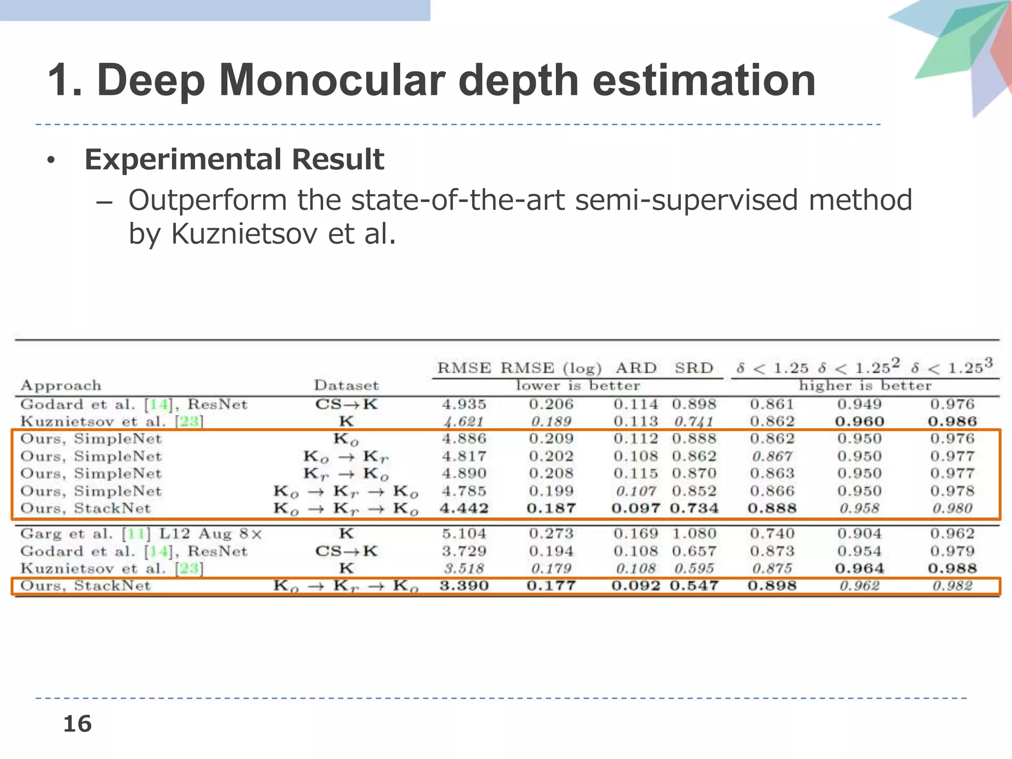
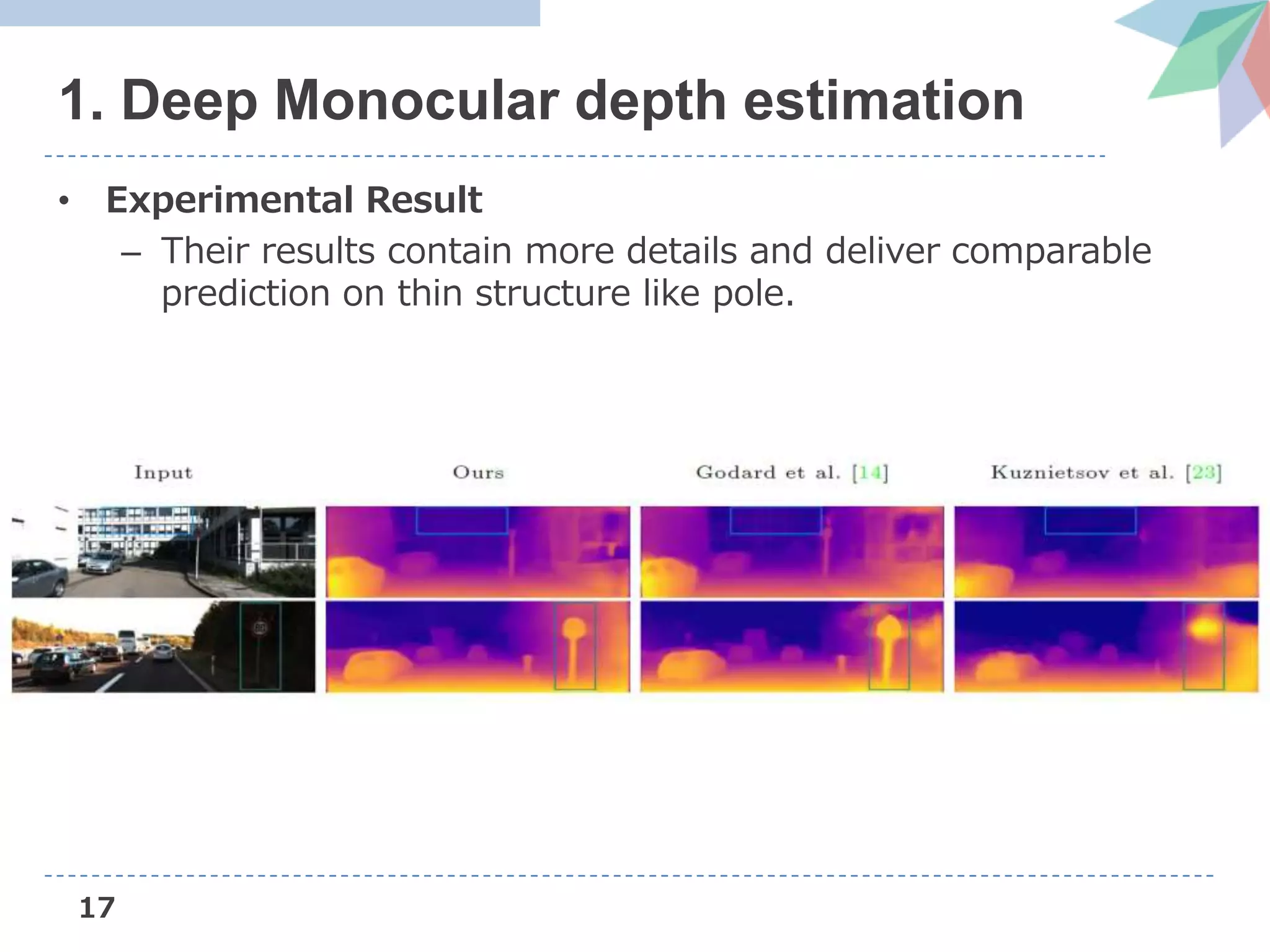
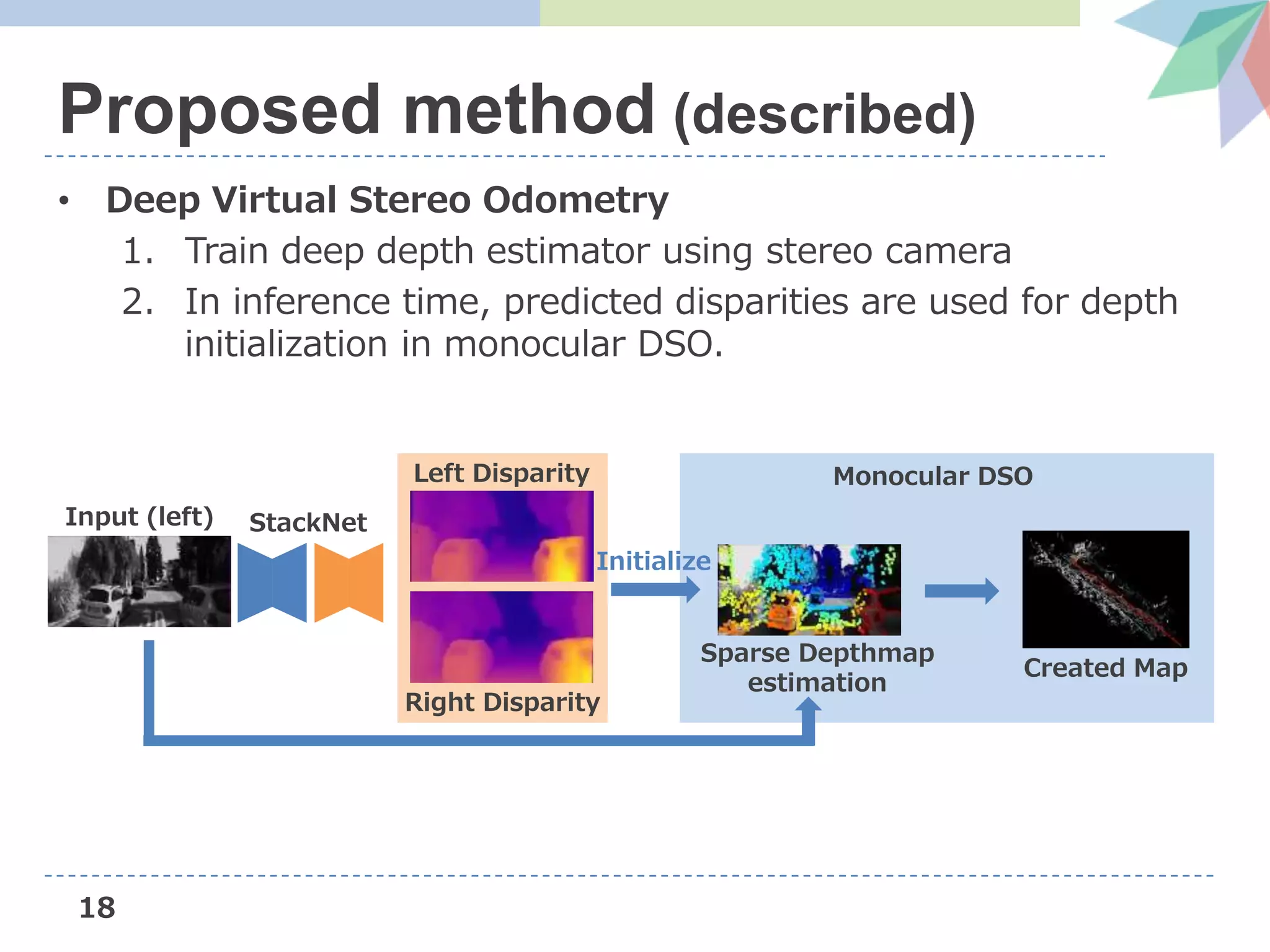
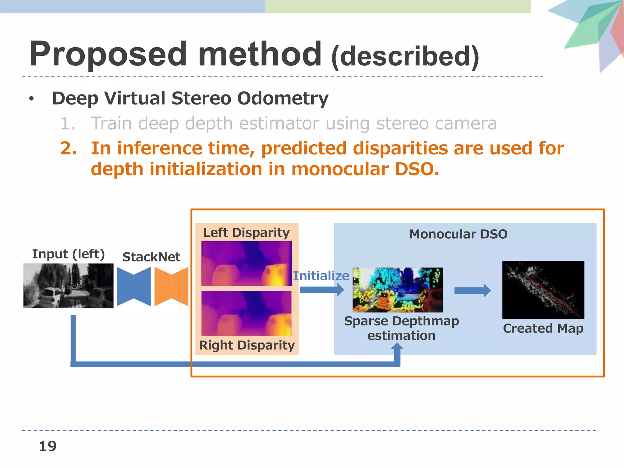
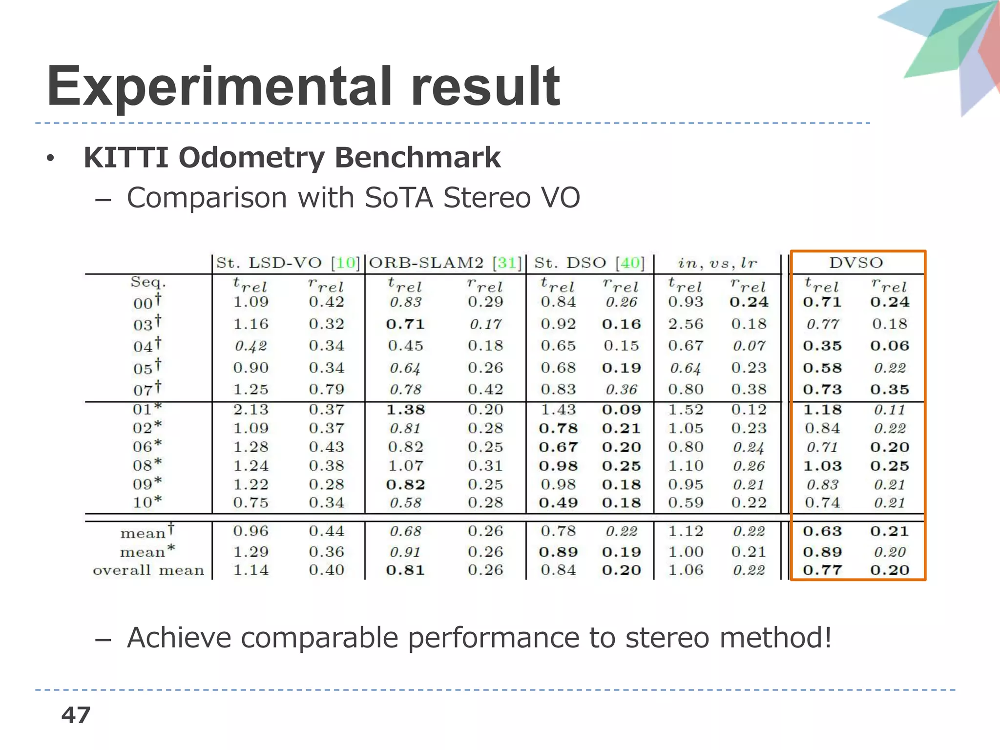
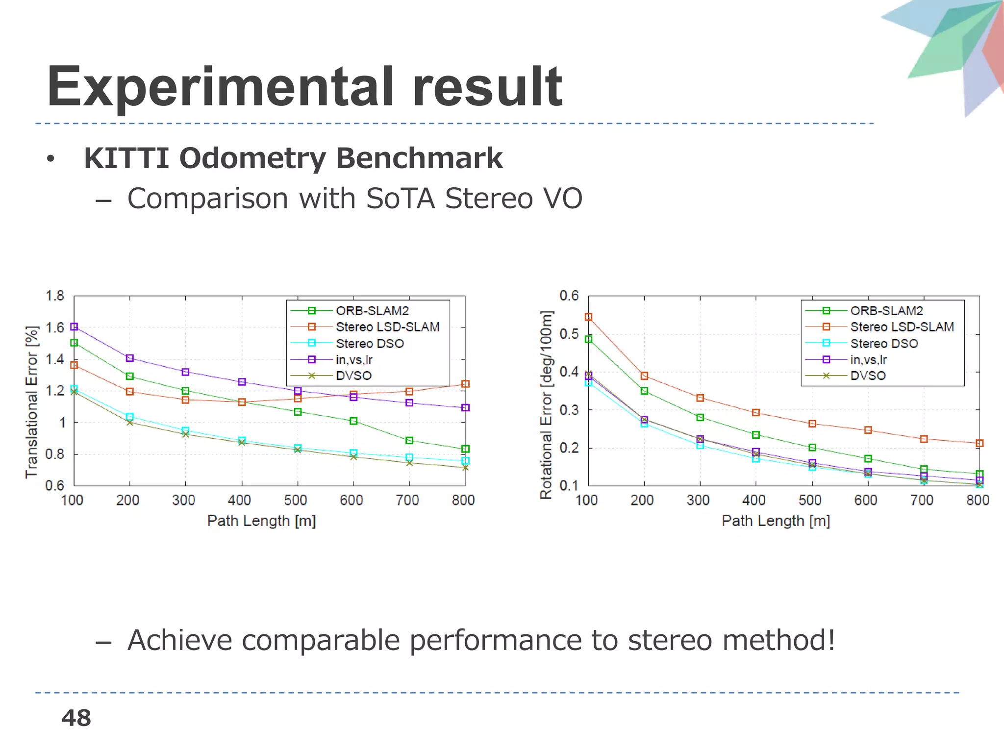
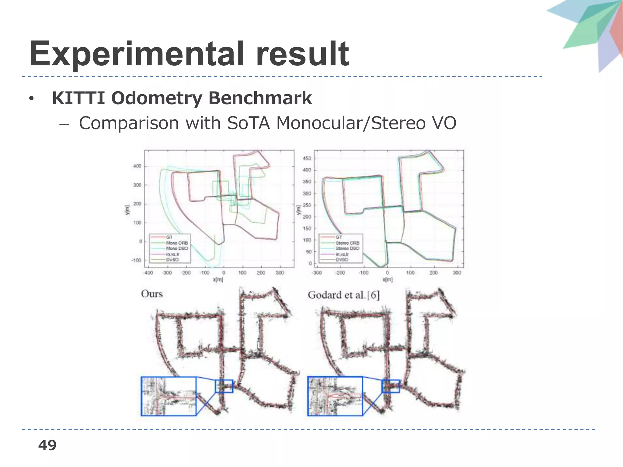
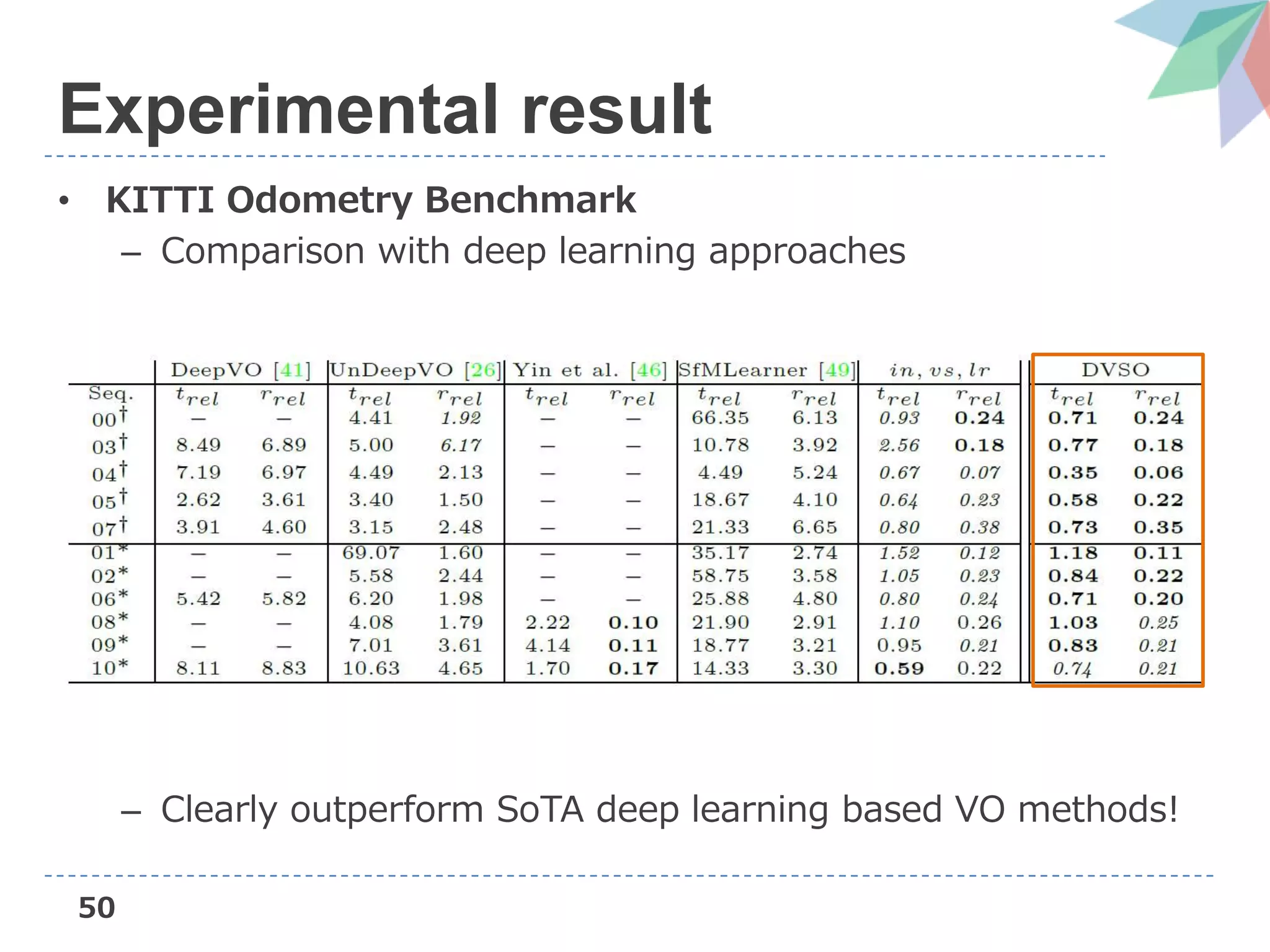
The document presents Deep Virtual Stereo Odometry (DVSO), a novel monocular visual odometry system that utilizes deep depth prediction to mitigate scale drift and improve the accuracy of 3D reconstruction. The approach trains a depth estimator using stereo camera inputs, which are then applied during inference with monocular cameras for depth initialization in Direct Sparse Odometry. Experimental results demonstrate that DVSO achieves performance comparable to stereo methods while outperforming state-of-the-art monocular visual odometry techniques.

1. Deep Virtual Stereo Odometry:
Leveraging Deep Depth Prediction for Monocular
Direct Sparse Odometry [ECCV2018(oral)]
The University of Tokyo
Aizawa Lab M1 Masaya Kaneko
論文読み会 @ AIST

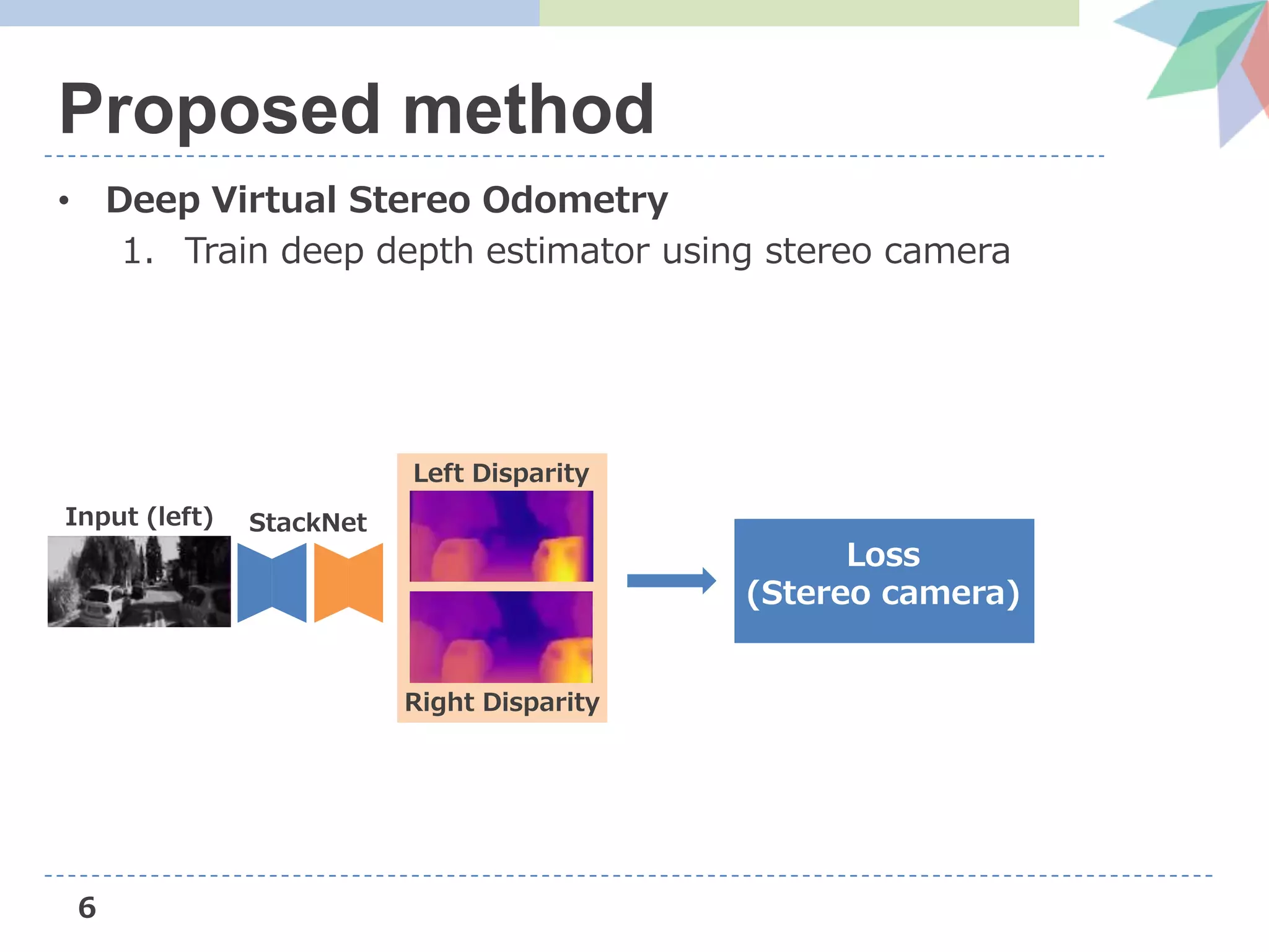
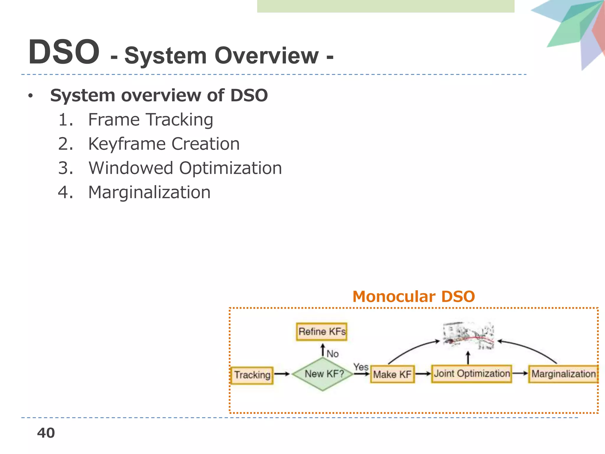
2. 1
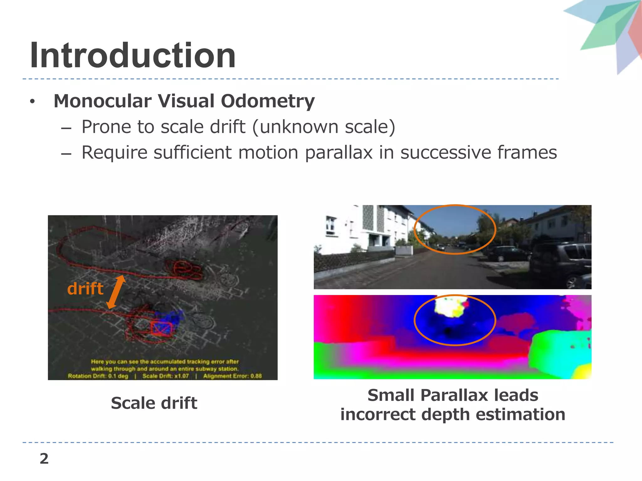
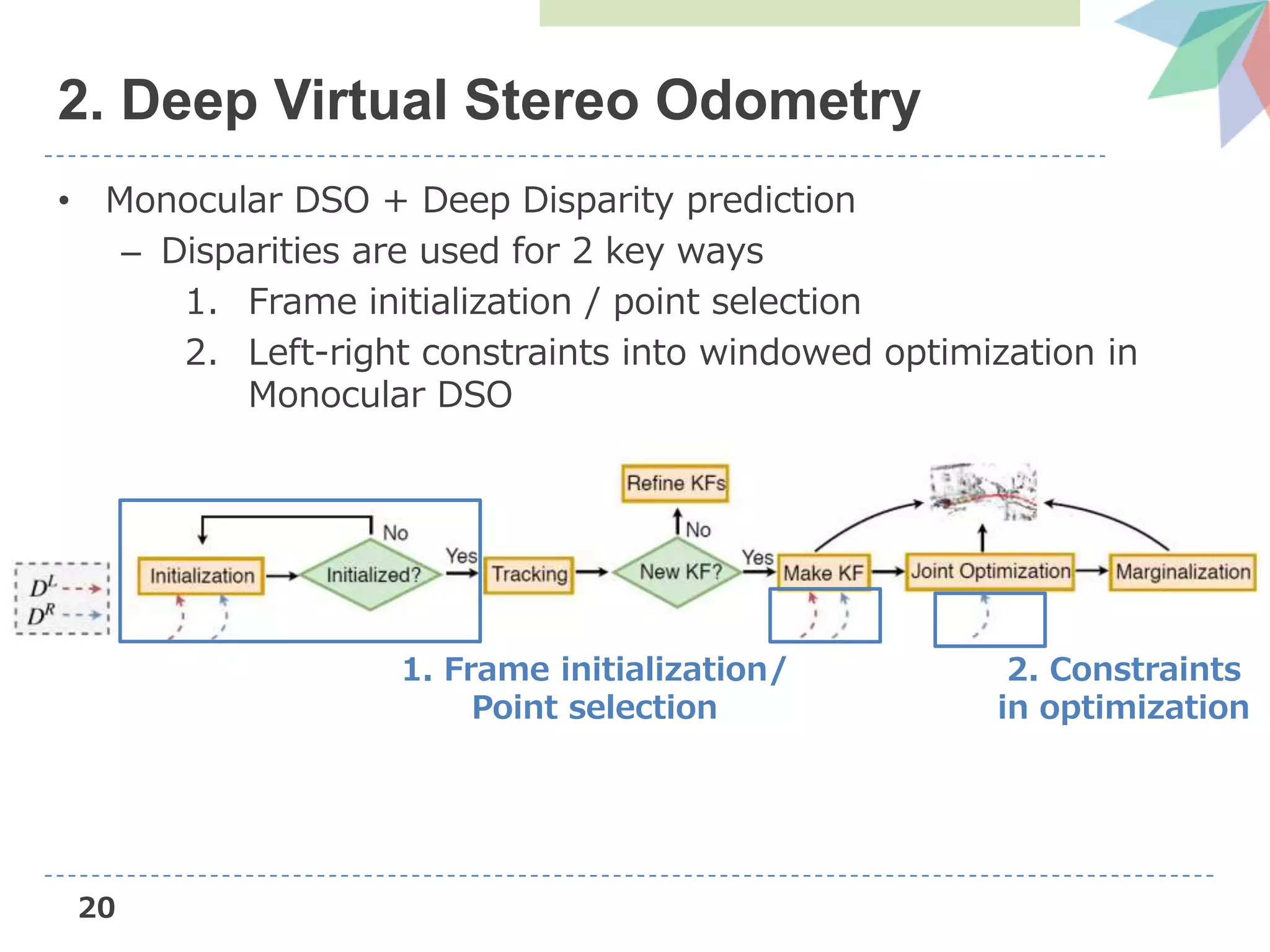
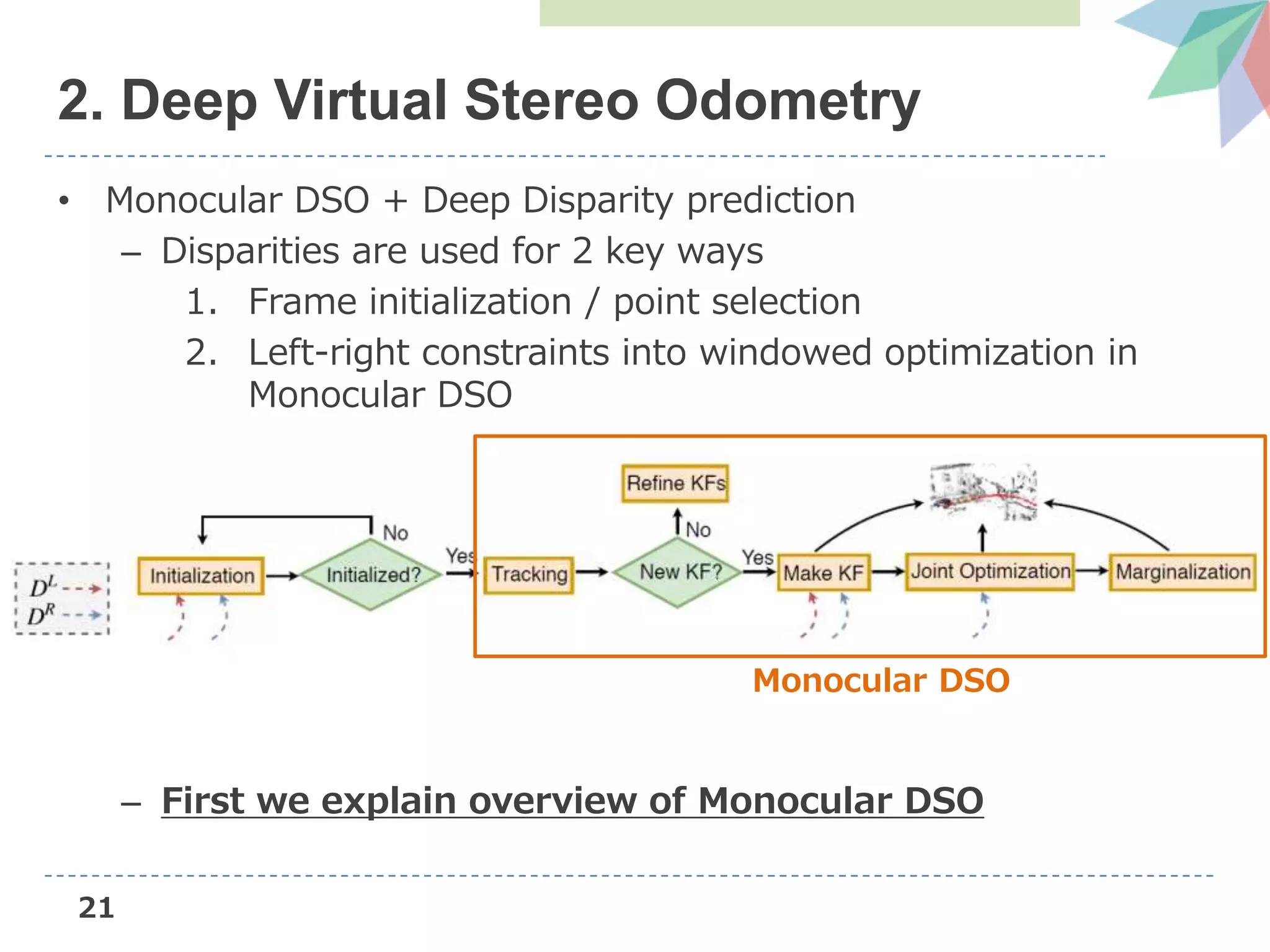
Introduction
• Monocular Visual Odometry
– Camera’s trajectory estimation and 3D reconstruction from
image sequences obtained by monocular camera
Direct Sparse Odometry [Engel+, PAMI’18]

3. 2
Introduction
• Monocular Visual Odometry
– Prone to scale drift (unknown scale)
– Require sufficient motion parallax in successive frames
Scale drift Small Parallax leads
incorrect depth estimation
drift

4. 3
Introduction
• Typically complex sensors are employed to avoid this issue.
– Active depth sensors (LiDAR, RGB-D camera)
– Stereo camera
• However, these sensors have following disadvantages.
– Require larger efforts in calibration
– Increase the cost of system
Velodyne
(https://velodynelidar.com/)
ZED
(https://www.stereolabs.com/)

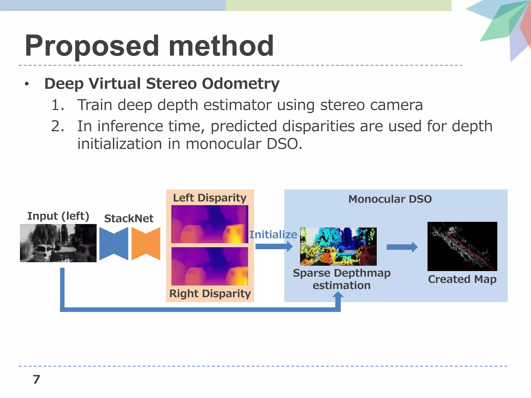
5. 4
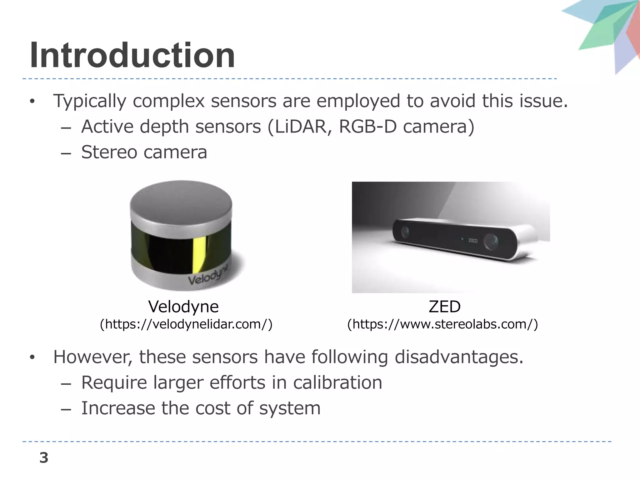
Introduction
• If a priori knowledge about environment is used, this issue
can be solved without complex sensors.
– Deep based approach like CNN-SLAM [Tateno+, CVPR’18]
– Now they propose a method to adapt this approach into
state-of-the-art VO, DSO (Direct Sparse Odometry).
https://drive.google.com/file/d/108CttbYiBqaI3b1jIJFTS26SzNfQqQNG/view

6. 5
Problem setting
• Requirements
– In inference time, you can only use monocular camera.
(for Monocular Visual Odometry)
– In train time, only inexpensive sensors are available.
• Mono/Stereo camera is ok.
• Active sensors are too costly to use.
Sensors Inference Train
Monocular camera 〇 〇
Stereo camera × 〇
Active sensors
(RGB-D, LiDAR)
× ×

7. • Deep Virtual Stereo Odometry
1. Train deep depth estimator using stereo camera
6
Proposed method
Loss
(Stereo camera)
Input (left)
Left Disparity
Right Disparity
StackNet

8. • Deep Virtual Stereo Odometry
1. Train deep depth estimator using stereo camera
2. In inference time, predicted disparities are used for depth
initialization in monocular DSO.
7
Proposed method
Monocular DSO
Sparse Depthmap
estimation
Created Map
Input (left)
Left Disparity
Right Disparity
Initialize
StackNet

9. • Deep Virtual Stereo Odometry
1. Train deep depth estimator using stereo camera
2. In inference time, predicted disparities are used for depth
initialization in monocular DSO.
8
Proposed method
Monocular DSO
Sparse Depthmap
estimation
Created Map
Input (left)
Left Disparity
Right Disparity
Initialize
StackNet

10. 9
1. Deep Monocular depth estimation
• 3 key ingredients
Network Architecture Loss Function
1. StackNet
2 stage refinement of the network
predictions in a stacked encoder-
decoder architecture
Input (left)
Left Disparity
Right Disparity
StackNet
3. Supervised learning
Use accurate sparse depth reconstruction
by Stereo DSO as GT
Left Disparity
Stereo DSO’s
Reconstructed result
2. Self-supervised learning
Photoconsistency in a stereo setup
𝐼𝑙𝑒𝑓𝑡
𝑑𝑖𝑠𝑝 𝑟𝑖𝑔ℎ𝑡
𝐼𝑟𝑒𝑐𝑜𝑛𝑠
𝑟𝑖𝑔ℎ𝑡
𝐼𝑟𝑒𝑐𝑜𝑛𝑠
𝑙𝑒𝑓𝑡
𝑑𝑖𝑠𝑝𝑙𝑒𝑓𝑡

11. 10
1. Deep Monocular depth estimation
• Network Architecture
– StackNet (SimpleNet + ResidualNet)

12. 11
1. Deep Monocular depth estimation
• Loss Function
– Linear combination of 5 terms in each image scale
1. Self-supervised loss
2. Supervised loss
3. Left-right disparity consistency loss
4. Disparity smoothness regularization
5. Occlusion regularization

13. 12
1. Deep Monocular depth estimation
• Loss Function
1. Self-supervised loss
• Measures the quality of the reconstructed images
𝐼𝑙𝑒𝑓𝑡
𝑑𝑖𝑠𝑝 𝑟𝑖𝑔ℎ𝑡
𝐼𝑟𝑒𝑐𝑜𝑛𝑠
𝑟𝑖𝑔ℎ𝑡
𝐼𝑟𝑒𝑐𝑜𝑛𝑠
𝑙𝑒𝑓𝑡
𝑑𝑖𝑠𝑝𝑙𝑒𝑓𝑡

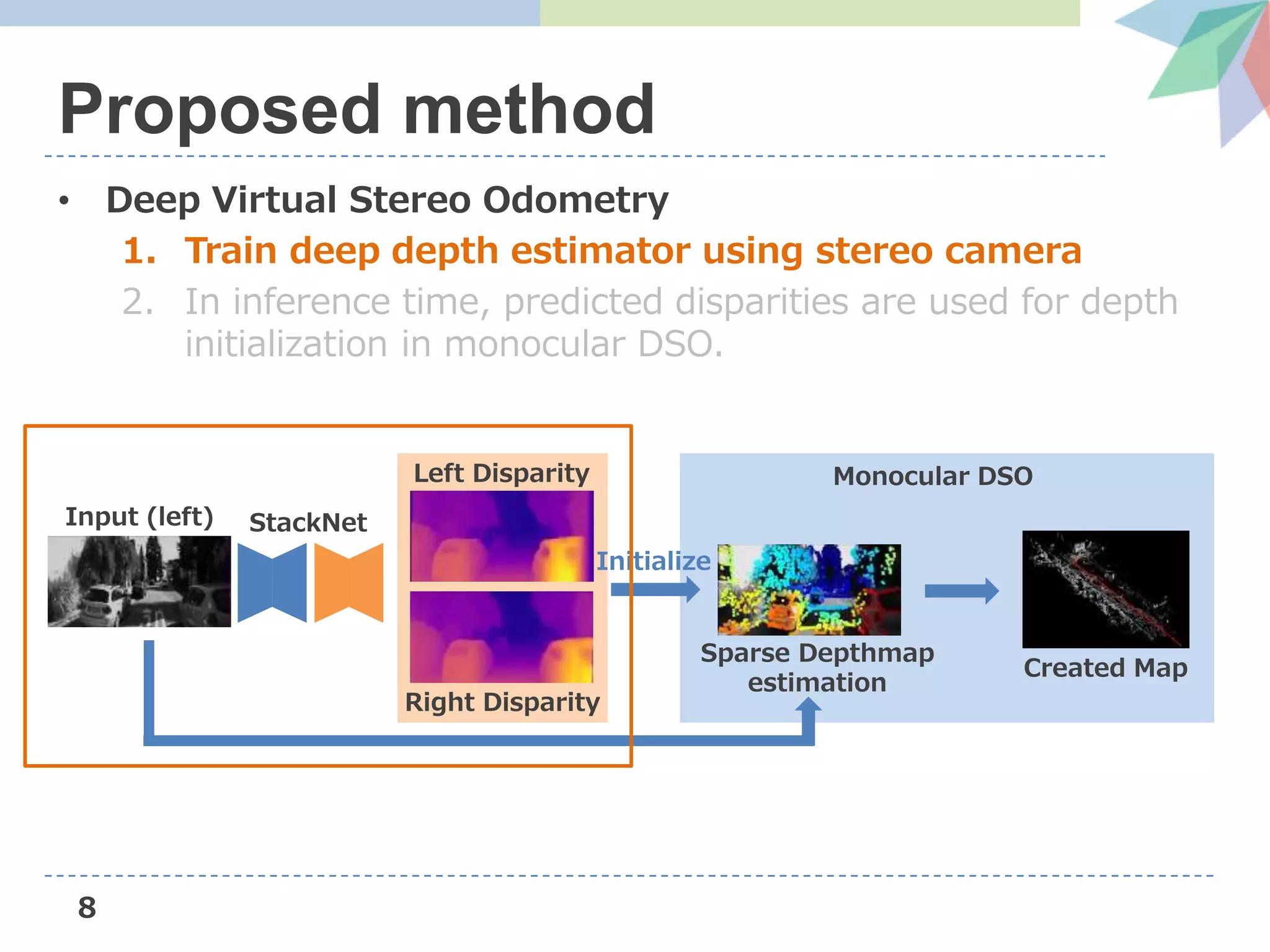
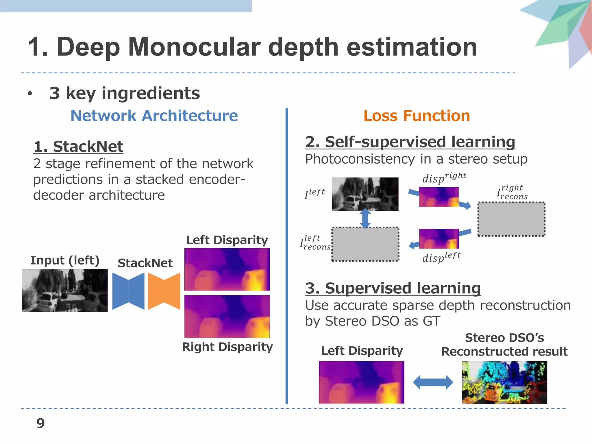
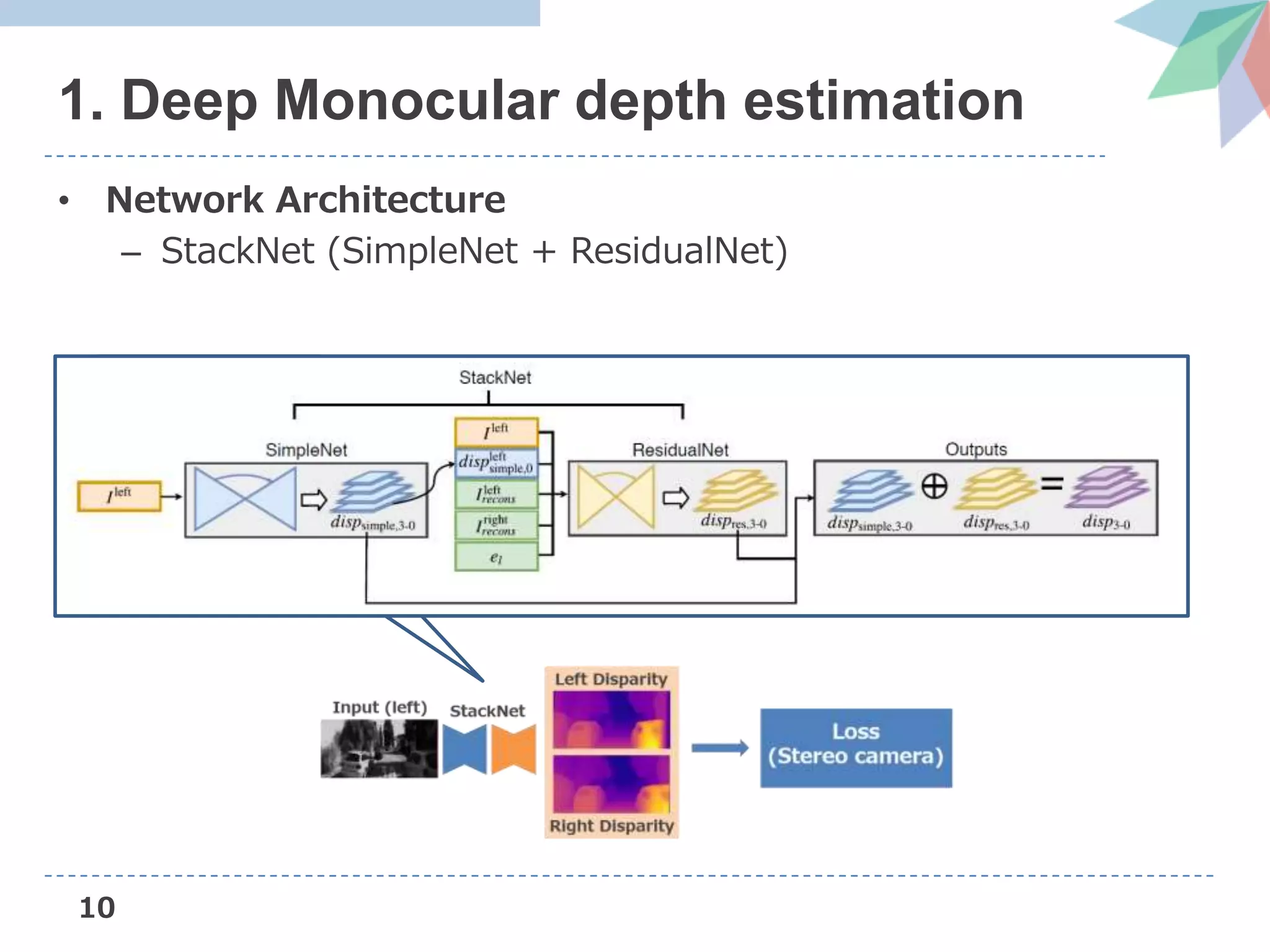
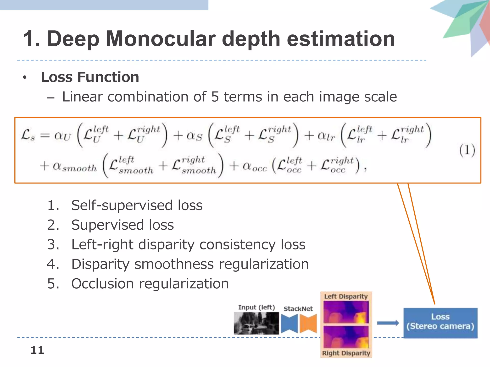
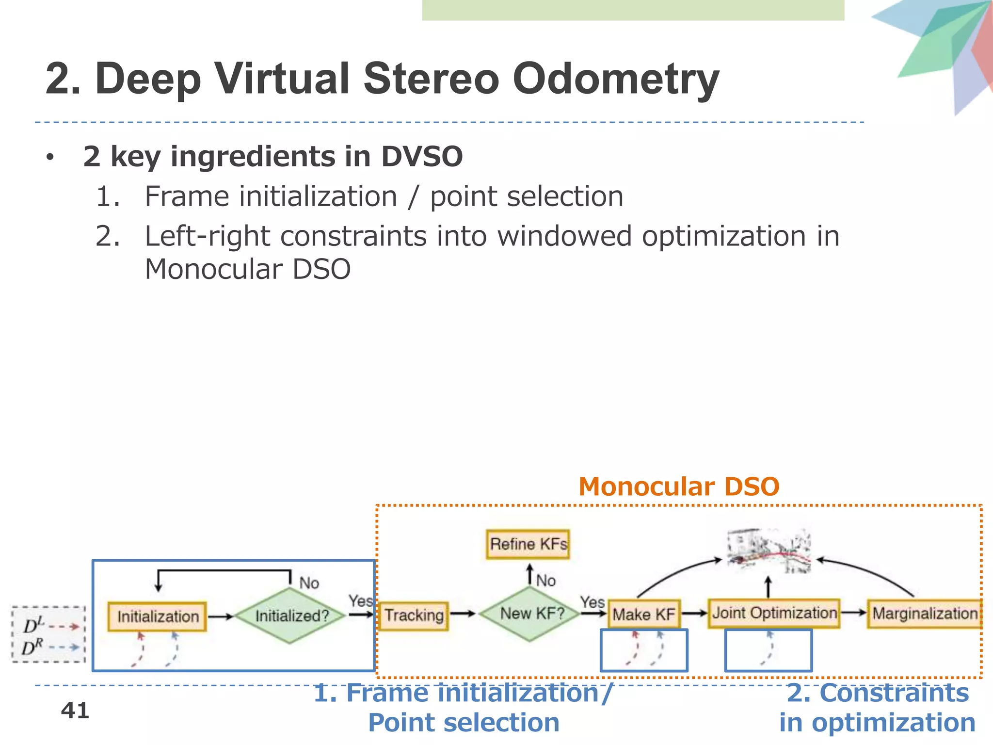
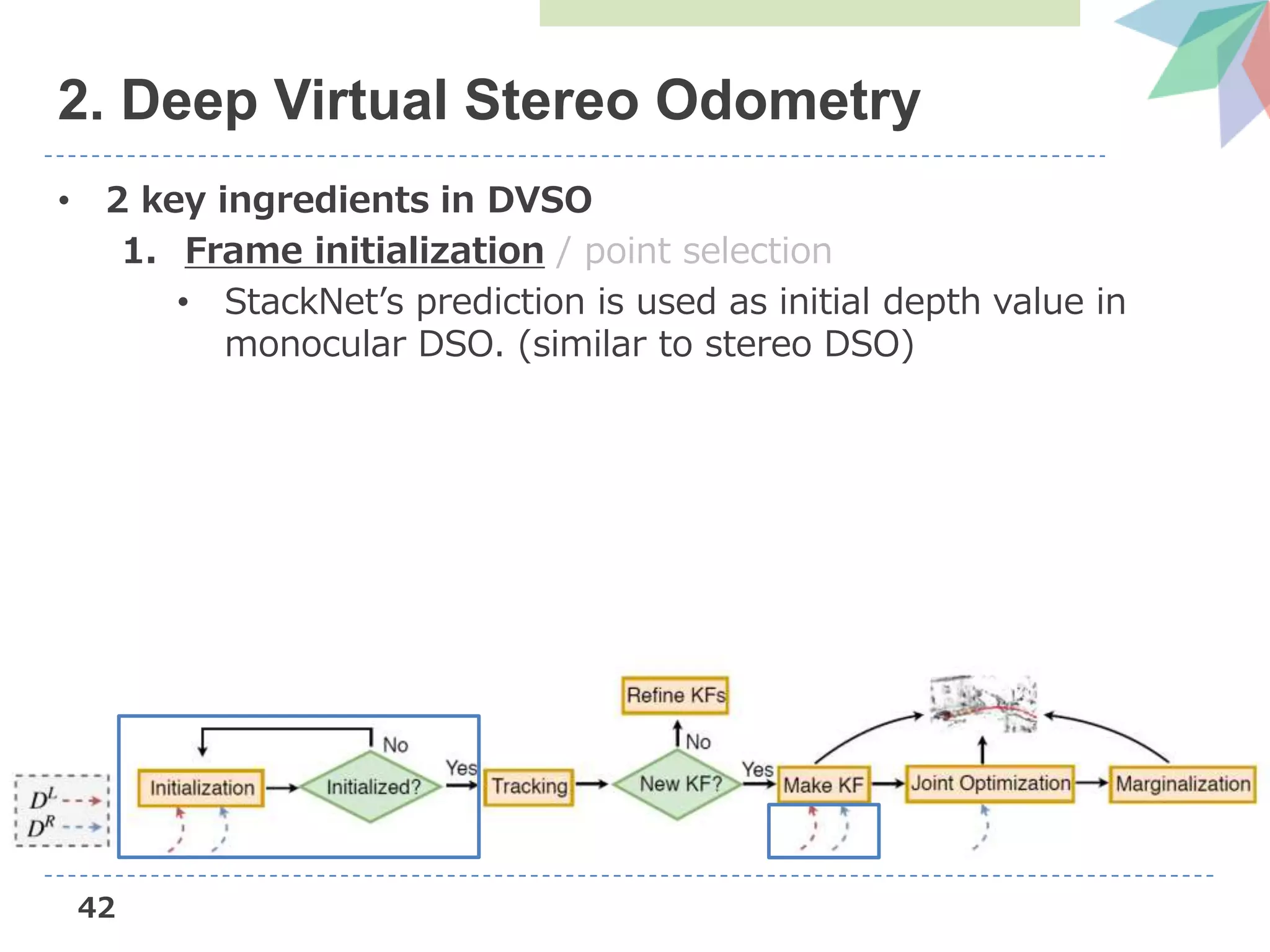
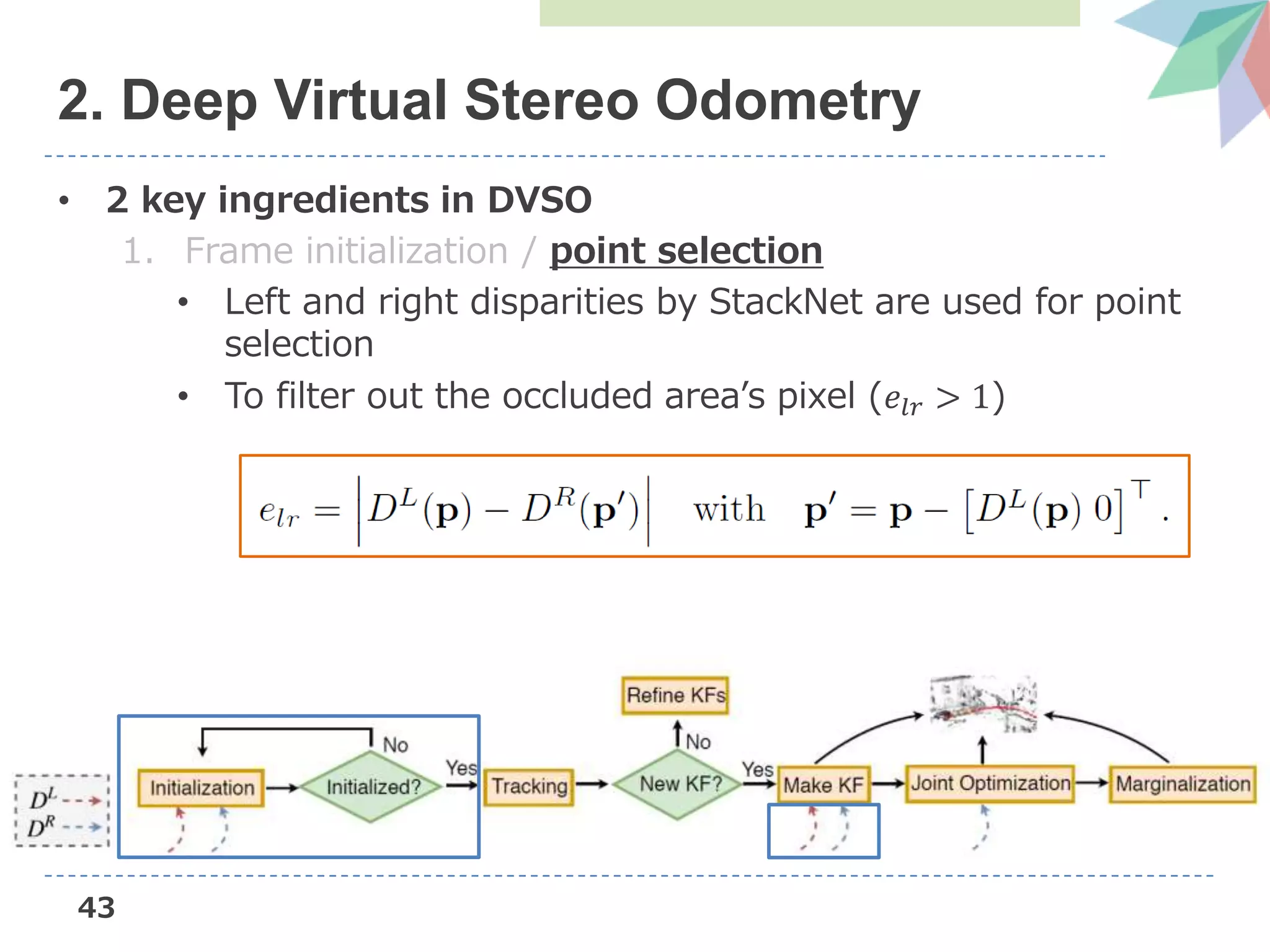
14. 13
1. Deep Monocular depth estimation
• Loss Function
2. Supervised loss
• Measures the deviation of the predicted disparity from
disparities estimated by Stereo DSO [Wang+, ICCV’17]
Left Disparity
Stereo DSO’s
Reconstructed result
Stereo DSO
(using Stereo camera)

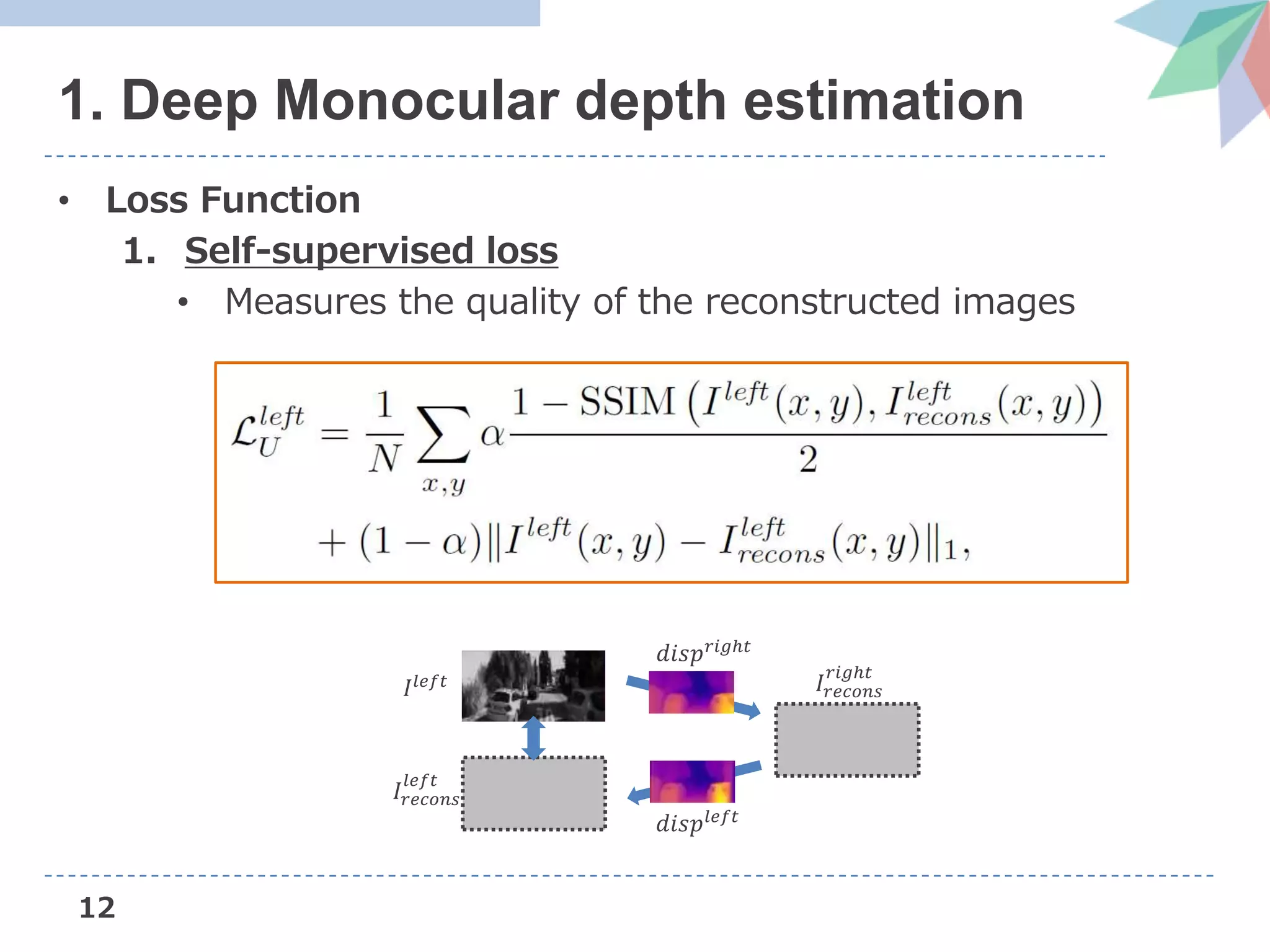
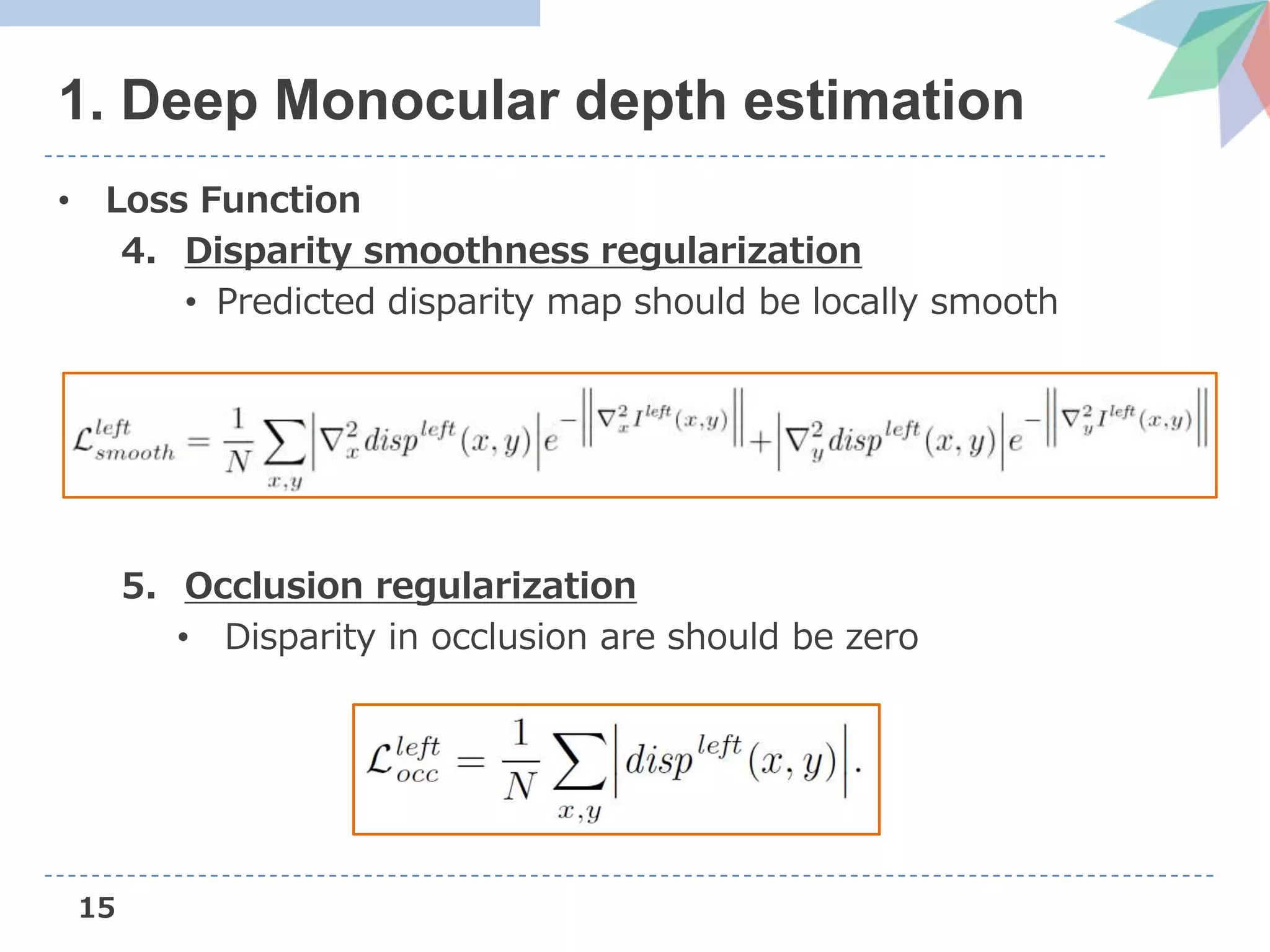
15. 14
1. Deep Monocular depth estimation
• Loss Function
3. Left-right disparity consistency loss
• Consistency loss proposed in MonoDepth [Godard+, CVPR’17]
𝐼𝑙𝑒𝑓𝑡
𝑑𝑖𝑠𝑝𝑙𝑒𝑓𝑡 𝑑𝑖𝑠𝑝 𝑟𝑖𝑔ℎ𝑡
𝐼 𝑟𝑖𝑔ℎ𝑡
𝑑𝑖𝑠𝑝𝑙𝑒𝑓𝑡

16. 15
1. Deep Monocular depth estimation
• Loss Function
4. Disparity smoothness regularization
• Predicted disparity map should be locally smooth
5. Occlusion regularization
• Disparity in occlusion are should be zero

17. 16
1. Deep Monocular depth estimation
• Experimental Result
– Outperform the state-of-the-art semi-supervised method
by Kuznietsov et al.

18. 17
1. Deep Monocular depth estimation
• Experimental Result
– Their results contain more details and deliver comparable
prediction on thin structure like pole.

19. • Deep Virtual Stereo Odometry
1. Train deep depth estimator using stereo camera
2. In inference time, predicted disparities are used for depth
initialization in monocular DSO.
18
Proposed method (described)
Monocular DSO
Sparse Depthmap
estimation
Created Map
Input (left)
Left Disparity
Right Disparity
Initialize
StackNet

20. • Deep Virtual Stereo Odometry
1. Train deep depth estimator using stereo camera
2. In inference time, predicted disparities are used for
depth initialization in monocular DSO.
19
Proposed method (described)
Monocular DSO
Sparse Depthmap
estimation
Created Map
Input (left)
Left Disparity
Right Disparity
Initialize
StackNet

21. 20
2. Deep Virtual Stereo Odometry
• Monocular DSO + Deep Disparity prediction
– Disparities are used for 2 key ways
1. Frame initialization / point selection
2. Left-right constraints into windowed optimization in
Monocular DSO
1. Frame initialization/
Point selection
2. Constraints
in optimization

22. 21
2. Deep Virtual Stereo Odometry
• Monocular DSO + Deep Disparity prediction
– Disparities are used for 2 key ways
1. Frame initialization / point selection
2. Left-right constraints into windowed optimization in
Monocular DSO
– First we explain overview of Monocular DSO
Monocular DSO

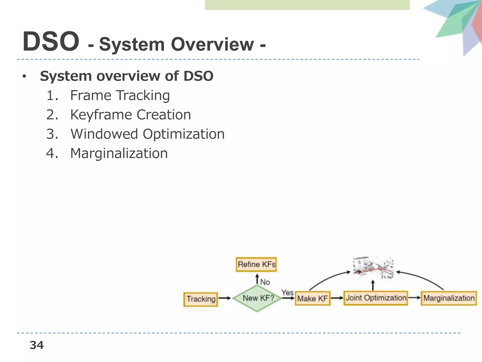
23. 22
DSO (Direct Sparse Odometry)
• Novel direct sparse Visual Odometry method
– Direct: seamless ability to use & reconstruct all points
instead of only corners
– Sparse: efficient, joint optimization of all parameters
Feature-based,
Sparse
Direct,
Semi-dense
Taking both approach’s benefits
[1] https://drive.google.com/file/d/108CttbYiBqaI3b1jIJFTS26SzNfQqQNG/view
LSD-SLAM [Engel+, ICCV’14] ORB-SLAM [Mur-Artal+, MVIGRO’14]

24. 23
• Direct sparse model
DSO - Model Formulation-
Target frame 𝐼′𝑗
(Pose 𝐓𝑗,
exposure time 𝒕𝑗)
𝒑
𝓝 𝒑
𝒑′Depth 1/𝑑 𝒑
Back-Projection
Π 𝑐
−1
Projection
Π 𝑐
Reference frame 𝐼′𝑖
(Pose 𝐓𝑖,
exposure time 𝒕𝑖)

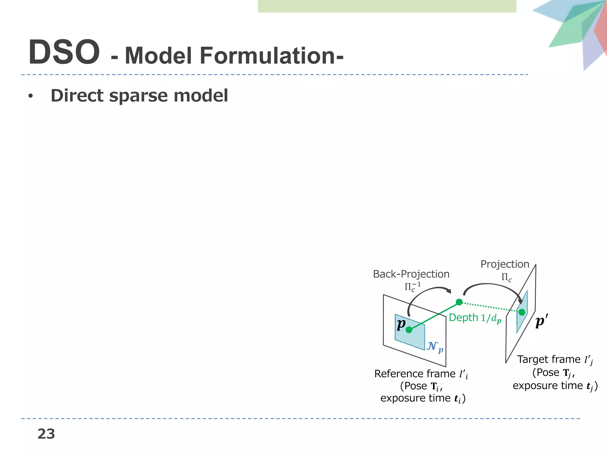
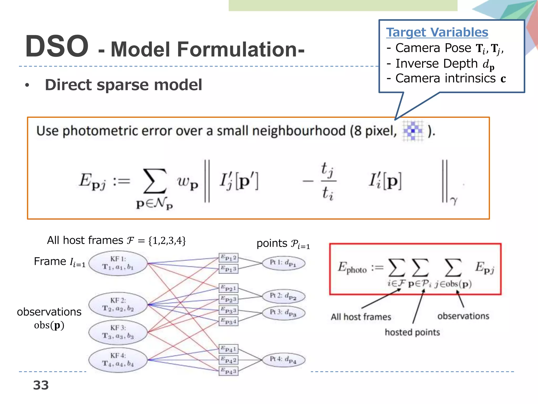
25. 24
• Direct sparse model
DSO - Model Formulation-
Target frame 𝐼′𝑗
(Pose 𝐓𝑗,
exposure time 𝒕𝑗)
𝒑
𝓝 𝒑
𝒑′Depth 1/𝑑 𝒑
Back-Projection
Π 𝑐
−1
Projection
Π 𝑐
Reference frame 𝐼′𝑖
(Pose 𝐓𝑖,
exposure time 𝒕𝑖)
𝓝 𝒑
[1] https://people.eecs.berkeley.edu/~chaene/cvpr17tut/SLAM.pdf

26. 25
• Direct sparse model
DSO - Model Formulation-
Target frame 𝐼′𝑗
(Pose 𝐓𝑗,
exposure time 𝒕𝑗)
𝒑
𝓝 𝒑
𝒑′Depth 1/𝑑 𝒑
Back-Projection
Π 𝑐
−1
Projection
Π 𝑐
Reference frame 𝐼′𝑖
(Pose 𝐓𝑖,
exposure time 𝒕𝑖)
𝓝 𝒑
Target Variables
- Camera Pose 𝐓𝑖, 𝐓𝑗,
- Inverse Depth 𝑑 𝐩
- Camera intrinsics 𝐜
[1] https://people.eecs.berkeley.edu/~chaene/cvpr17tut/SLAM.pdf

27. 26
• Direct sparse model
DSO - Model Formulation-
Target frame 𝐼′𝑗
(Pose 𝐓𝑗,
exposure time 𝒕𝑗)
𝒑
𝓝 𝒑
𝒑′Depth 1/𝑑 𝒑
Back-Projection
Π 𝑐
−1
Projection
Π 𝑐
Reference frame 𝐼′𝑖
(Pose 𝐓𝑖,
exposure time 𝒕𝑖)
𝓝 𝒑
Target Variables
- Camera Pose 𝐓𝑖, 𝐓𝑗,
- Inverse Depth 𝑑 𝐩
- Camera intrinsics 𝐜
Error between irradiance 𝑩 = 𝑰/𝒕
[1] https://people.eecs.berkeley.edu/~chaene/cvpr17tut/SLAM.pdf

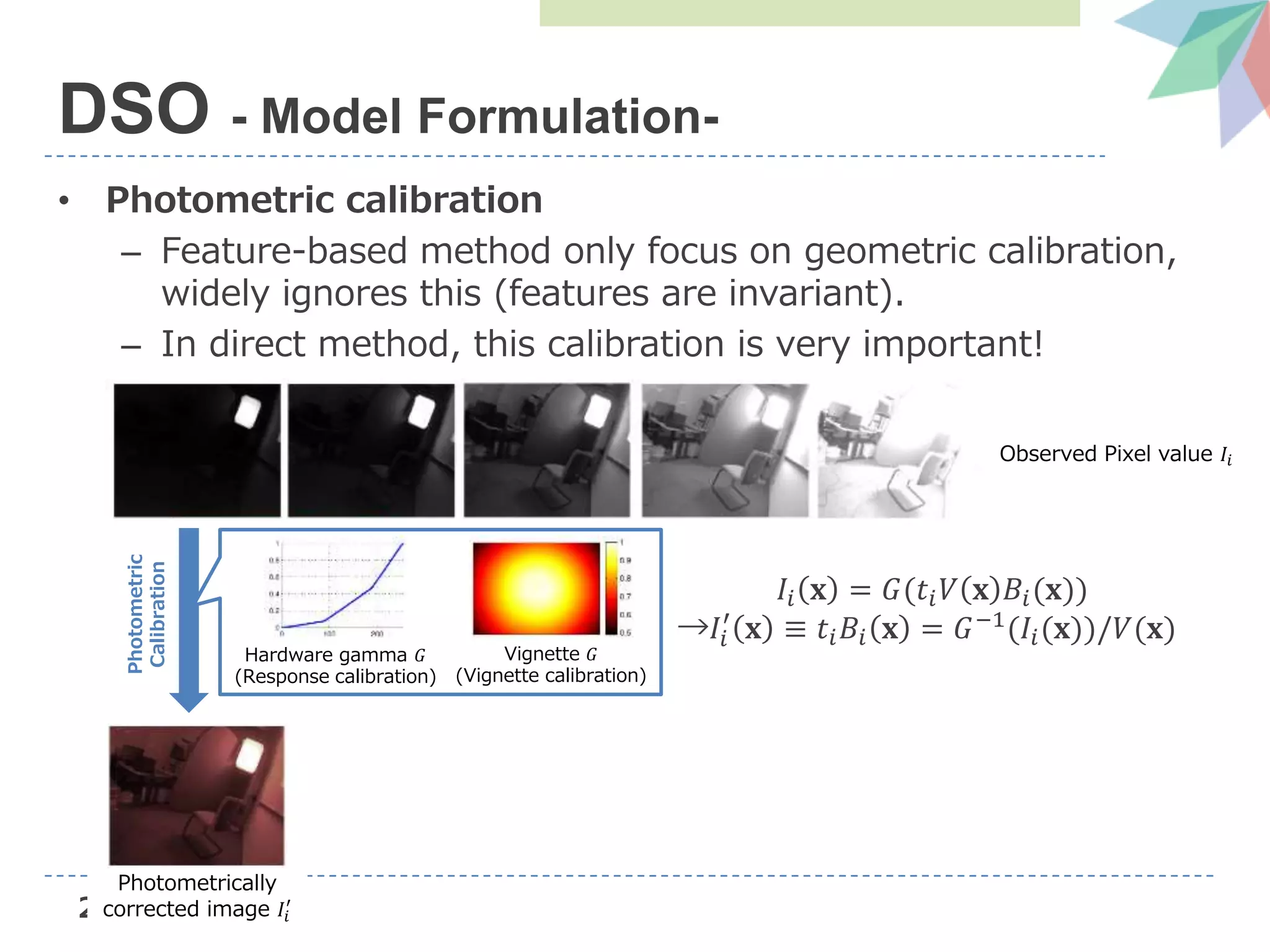
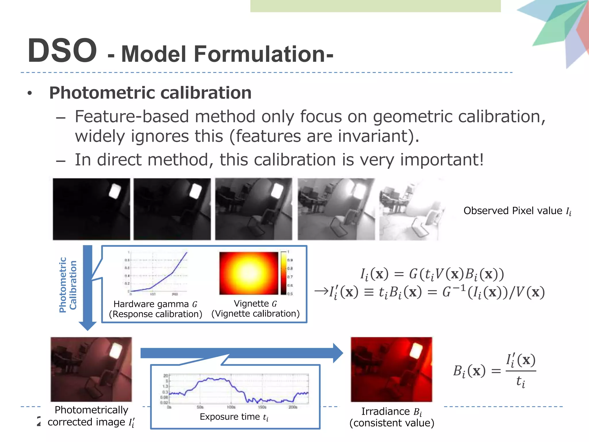
28. 27
• Photometric calibration
– Feature-based method only focus on geometric calibration,
widely ignores this (features are invariant).
– In direct method, this calibration is very important!
DSO - Model Formulation-
Observed Pixel value 𝐼𝑖
[1] https://people.eecs.berkeley.edu/~chaene/cvpr17tut/SLAM.pdf

29. 28
• Photometric calibration
– Feature-based method only focus on geometric calibration,
widely ignores this (features are invariant).
– In direct method, this calibration is very important!
DSO - Model Formulation-
Observed Pixel value 𝐼𝑖
Photometric
Calibration
Hardware gamma 𝐺
(Response calibration)
Vignette 𝐺
(Vignette calibration)
Photometrically
corrected image 𝐼𝑖
′
𝐼𝑖 𝐱 = 𝐺(𝑡𝑖 𝑉 𝐱 𝐵𝑖(𝐱))
→𝐼𝑖
′
𝐱 ≡ 𝑡𝑖 𝐵𝑖 𝐱 = 𝐺−1
(𝐼𝑖(𝐱))/𝑉(𝐱)

30. 29
• Photometric calibration
– Feature-based method only focus on geometric calibration,
widely ignores this (features are invariant).
– In direct method, this calibration is very important!
DSO - Model Formulation-
Observed Pixel value 𝐼𝑖
Photometric
Calibration
Hardware gamma 𝐺
(Response calibration)
Vignette 𝐺
(Vignette calibration)
Irradiance 𝐵𝑖
(consistent value)
𝐼𝑖 𝐱 = 𝐺(𝑡𝑖 𝑉 𝐱 𝐵𝑖(𝐱))
→𝐼𝑖
′
𝐱 ≡ 𝑡𝑖 𝐵𝑖 𝐱 = 𝐺−1
(𝐼𝑖(𝐱))/𝑉(𝐱)
Photometrically
corrected image 𝐼𝑖
′ Exposure time 𝑡𝑖
𝐵𝑖 𝐱 =
𝐼𝑖
′
(𝐱)
𝑡𝑖

31. 30
• Direct sparse model
DSO - Model Formulation-
Target frame 𝐼′𝑗
(Pose 𝐓𝑗,
exposure time 𝒕𝑗)
𝒑
𝓝 𝒑
𝒑′Depth 1/𝑑 𝒑
Back-Projection
Π 𝑐
−1
Projection
Π 𝑐
Reference frame 𝐼′𝑖
(Pose 𝐓𝑖,
exposure time 𝒕𝑖)
𝓝 𝒑
Error between irradiance 𝑩 = 𝑰/𝒕
[1] https://people.eecs.berkeley.edu/~chaene/cvpr17tut/SLAM.pdf

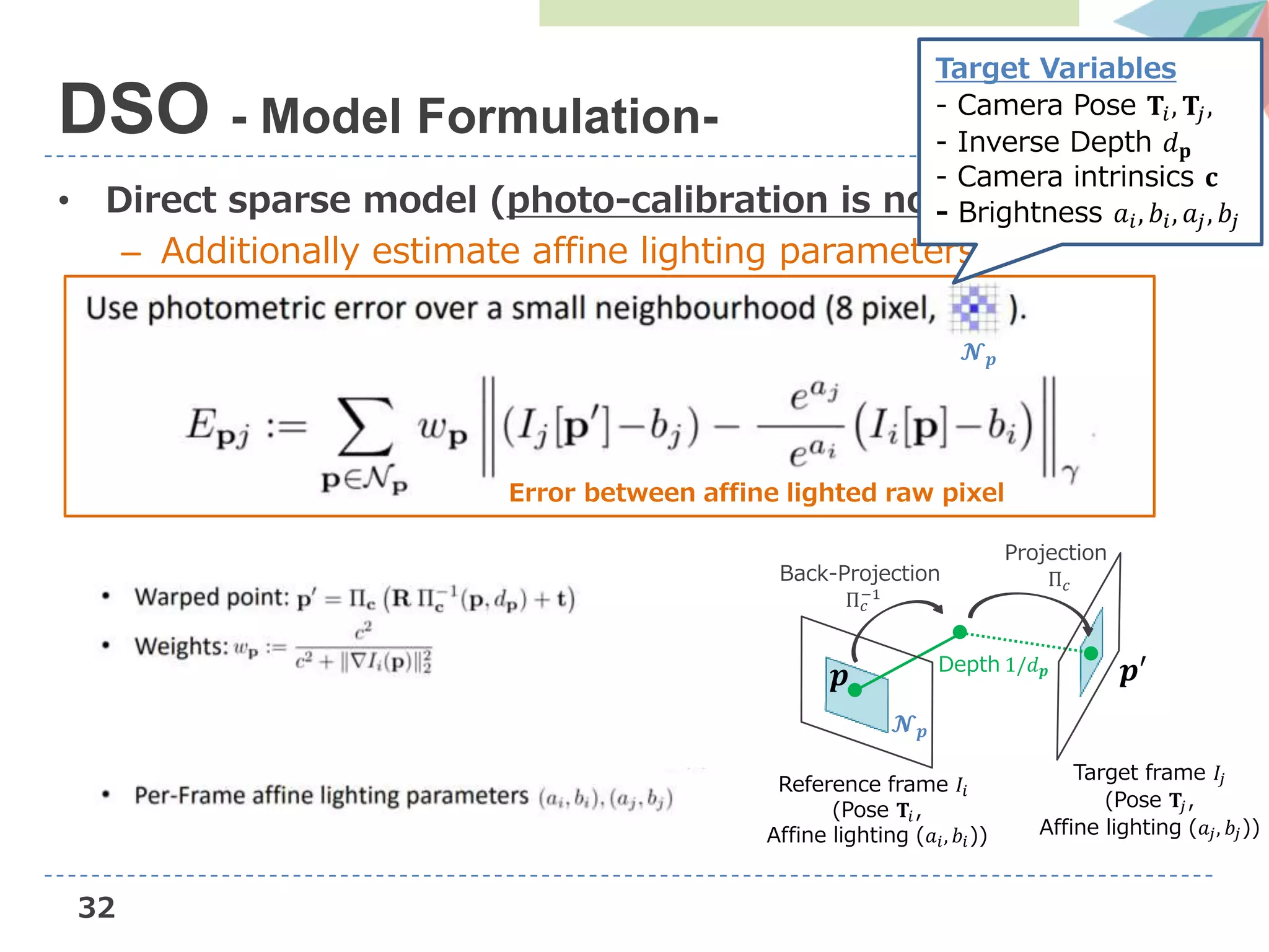
32. 31
• Direct sparse model (photo-calibration is not available)
– Additionally estimate affine lighting parameters
DSO - Model Formulation-
Reference frame 𝐼𝑖
(Pose 𝐓𝑖,
Affine lighting (𝑎𝑖, 𝑏𝑖))
Target frame 𝐼𝑗
(Pose 𝐓𝑗,
Affine lighting (𝑎𝑗, 𝑏𝑗))
𝒑
𝓝 𝒑
𝒑′Depth 1/𝑑 𝒑
Back-Projection
Π 𝑐
−1
Projection
Π 𝑐
𝓝 𝒑
Error between affine lighted raw pixel
[1] https://people.eecs.berkeley.edu/~chaene/cvpr17tut/SLAM.pdf

33. 32
• Direct sparse model (photo-calibration is not available)
– Additionally estimate affine lighting parameters
DSO - Model Formulation-
Reference frame 𝐼𝑖
(Pose 𝐓𝑖,
Affine lighting (𝑎𝑖, 𝑏𝑖))
Target frame 𝐼𝑗
(Pose 𝐓𝑗,
Affine lighting (𝑎𝑗, 𝑏𝑗))
𝒑
𝓝 𝒑
𝒑′Depth 1/𝑑 𝒑
Back-Projection
Π 𝑐
−1
Projection
Π 𝑐
𝓝 𝒑
Error between affine lighted raw pixel
Target Variables
- Camera Pose 𝐓𝑖, 𝐓𝑗,
- Inverse Depth 𝑑 𝐩
- Camera intrinsics 𝐜
- Brightness 𝑎𝑖, 𝑏𝑖, 𝑎𝑗, 𝑏𝑗

34. 33
• Direct sparse model
DSO - Model Formulation-
All host frames ℱ = {1,2,3,4}
Frame 𝐼𝑖=1
points 𝒫𝑖=1
observations
obs(𝐩)
Target Variables
- Camera Pose 𝐓𝑖, 𝐓𝑗,
- Inverse Depth 𝑑 𝐩
- Camera intrinsics 𝐜

35. 34
• System overview of DSO
1. Frame Tracking
2. Keyframe Creation
3. Windowed Optimization
4. Marginalization
DSO - System Overview -

36. 35
• System overview of DSO
1. Frame Tracking
2. Keyframe Creation
3. Windowed Optimization
4. Marginalization
DSO - System Overview -
Tracking + Depth estimation
- From active 𝑁𝑓(= 7) Keyframes
Multi-scale Image Pyramid
+ constant motion model

37. 36
• System overview of DSO
1. Frame Tracking
2. Keyframe Creation
3. Windowed Optimization
4. Marginalization
DSO - System Overview -
Tracking + Depth estimation
- Frame keeps 𝑁 𝑝 = 2000 points
1. Well distributed in an image ?
2. High image gradient magnitude ?
Point selection’s Two criteria

38. 37
• System overview of DSO
1. Frame Tracking
2. Keyframe Creation
3. Windowed Optimization
4. Marginalization
DSO - System Overview -
Whether KF is required or not ?
- Similar strategy to ORB-SLAM
1. In the view field ?
2. Occlusion ?
3. Camera exposure time?
Three criteria
If these conditions are met, tracked
frame is inserted as Keyframe.

39. • System overview of DSO
1. Frame Tracking
2. Keyframe Creation
3. Windowed Optimization
4. Marginalization
38
DSO - System Overview -
Windowed optimization (BA)
- Minimize Photometric error from
active Keyframes

40. • System overview of DSO
1. Frame Tracking
2. Keyframe Creation
3. Windowed Optimization
4. Marginalization
39
DSO - System Overview -
Marginalization
- Old variables are removed to
avoid too much computation
- Schur complement
Black : marginalized points

41. 40
• System overview of DSO
1. Frame Tracking
2. Keyframe Creation
3. Windowed Optimization
4. Marginalization
DSO - System Overview -
Monocular DSO

42. 41
• 2 key ingredients in DVSO
1. Frame initialization / point selection
2. Left-right constraints into windowed optimization in
Monocular DSO
2. Deep Virtual Stereo Odometry
1. Frame initialization/
Point selection
2. Constraints
in optimization
Monocular DSO

43. 42
• 2 key ingredients in DVSO
1. Frame initialization / point selection
• StackNet’s prediction is used as initial depth value in
monocular DSO. (similar to stereo DSO)
2. Deep Virtual Stereo Odometry

44. 43
• 2 key ingredients in DVSO
1. Frame initialization / point selection
• Left and right disparities by StackNet are used for point
selection
• To filter out the occluded area’s pixel (𝑒𝑙𝑟 > 1)
2. Deep Virtual Stereo Odometry

45. 44
• 2 key ingredients in DVSO
2. Additional Constraints in Optimization
• Monocular DSO’s total energy (described)
2. Deep Virtual Stereo Odometry
→

46. 45
• 2 key ingredients in DVSO
2. Additional Constraints in Optimization
• Introduce a novel virtual stereo term for each point
• To check whether optimized depth is consistent with
the disparity prediction of StackNet.
2. Deep Virtual Stereo Odometry

47. 46
• 2 key ingredients in DVSO
2. Additional Constraints in Optimization
• Total energy is summation of original error and virtual
stereo term
2. Deep Virtual Stereo Odometry
Original errorVirtual stereo term

48. 47
Experimental result
• KITTI Odometry Benchmark
– Comparison with SoTA Stereo VO
– Achieve comparable performance to stereo method!

49. 48
Experimental result
• KITTI Odometry Benchmark
– Comparison with SoTA Stereo VO
– Achieve comparable performance to stereo method!

50. 49
Experimental result
• KITTI Odometry Benchmark
– Comparison with SoTA Monocular/Stereo VO

51. 50
Experimental result
• KITTI Odometry Benchmark
– Comparison with deep learning approaches
– Clearly outperform SoTA deep learning based VO methods!

52. 51
Experimental result
• KITTI Odometry Benchmark
– Localization and Mapping Result

53. 52
Conclusion
• They present a novel monocular VO system, DVSO.
– Recover metric scale and Reduce scale drift with only a
single camera
– Outperform SoTA monocular VO
– Achieve comparable results to stereo VO
• Future work
– Fine-tune of the network inside the odometry pipeline end-
to-end.
– Investigate how much proposed approach can generalize
to other camera and environments