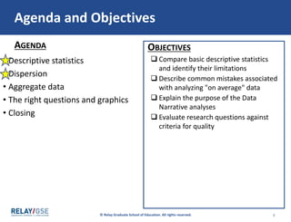
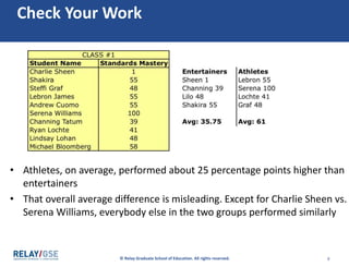
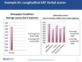
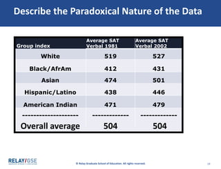
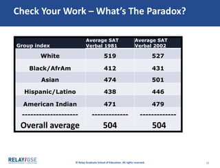
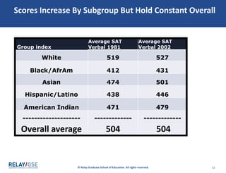
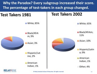
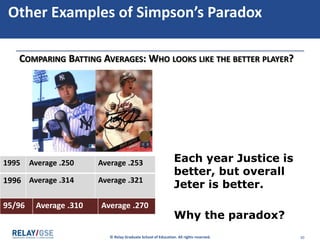
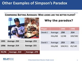
© Relay Graduate School of Education. All rights reserved. 1
AGGREGATE DATA
© Relay Graduate School of Education. All rights reserved. 22
AGENDA OBJECTIVES
Agenda and Objectives
• Descriptive statistics
• Dispersion
• Aggregate data
• The right questions and graphics
• Closing
 Compare basic descriptive statistics
and identify their limitations
 Describe common mistakes associated
with analyzing "on average" data
 Explain the purpose of the Data
Narrative analyses
 Evaluate research questions against
criteria for quality
2 2
© Relay Graduate School of Education. All rights reserved. 33
In the last activity, we
finished reviewing our
tree of statistical
terminology.
Now let’s apply that
knowledge!
© Relay Graduate School of Education. All rights reserved. 44
Aggregated Data
© Relay Graduate School of Education. All rights reserved. 5
Entertainers vs. Athletes for Class #1
• Who did better? How much better?
• Should we be worried about the lower-performing group? Why, why not?
• If you were the principal, would you intervene on behalf of the lower-
performing group? Is this teacher disfavoring entertainers?
Click ahead when
you’ve completed the
appropriate section
of your Handout
© Relay Graduate School of Education. All rights reserved. 7
Check Your Work
© Relay Graduate School of Education. All rights reserved. 8
Check Your Work
• Athletes, on average, performed about 25 percentage points higher than
entertainers
• That overall average difference is misleading. Except for Charlie Sheen vs.
Serena Williams, everybody else in the two groups performed similarly
© Relay Graduate School of Education. All rights reserved. 99
Statistical finding
vs.
Interesting finding
© Relay Graduate School of Education. All rights reserved. 1010
Statistical finding
vs.
Interesting finding
Athletes performed better than
entertainers. But the difference was
really just because Charlie Sheen
scored a 1 and Serena a 100.
© Relay Graduate School of Education. All rights reserved. 1111
Statistically significant
vs.
Practically significant
Not every statistical finding has any
practical purpose. A number is just a
number without any other context.
© Relay Graduate School of Education. All rights reserved. 1212
Speaking of…
“Statistical significance”
© Relay Graduate School of Education. All rights reserved. 13
Misuse of the Term “Statistically Significant”
The word "significant", in this sense, does not mean "large" or
"important" as it does in the everyday use of the word.
http://xkcd.com/539/
© Relay Graduate School of Education. All rights reserved. 1414
Statistical significance
The Data Narrative is NOT a test of
statistical significance! It’s an
exploration of your data. It’s a
report and analysis. It is NOT
statistical modeling.
© Relay Graduate School of Education. All rights reserved. 15
Correct use of the Term “Statistically Significant”
• Statistically significant, in the statistical sense, refers to something that is
unlikely to have occurred by chance. Like a scientific experiment
performed in a laboratory setting.
© Relay Graduate School of Education. All rights reserved. 1616
CORRELATION CAUSATION
Unless you're using randomized trials and
experimentation, in the statistical world,
you cannot say that something caused
something else. You can say that two
things are 'related', or may be
'contributing factors', but not they caused
each other.
© Relay Graduate School of Education. All rights reserved. 1717
Simpson’s Paradox:
Why even an average of
1.5 years of growth is not
necessarily good enough
© Relay Graduate School of Education. All rights reserved. 18
Example #1: Longitudinal SAT Verbal scores
Newspaper headlines:
Average scores don’t improve!
200
240
280
320
360
400
440
480
520
560
Overall
Average SAT
Verbal 1981
Average SAT
Verbal 2002
Behind the scenes:
Scores increases within every racial subgroup
200
240
280
320
360
400
440
480
520
560
Average
Verbal SAT
1981
Average
Verbal SAT
2002
© Relay Graduate School of Education. All rights reserved. 19
Describe the Paradoxical Nature of the Data
Group index
Average SAT
Verbal 1981
Average SAT
Verbal 2002
White 519 527
Black/AfrAm 412 431
Asian 474 501
Hispanic/Latino 438 446
American Indian 471 479
--------------------
Overall average
-------------
504
-------------
504
Click ahead when
you’ve completed the
appropriate section
of your Handout
© Relay Graduate School of Education. All rights reserved. 21
Check Your Work – What’s The Paradox?
Group index
Average SAT
Verbal 1981
Average SAT
Verbal 2002
White 519 527
Black/AfrAm 412 431
Asian 474 501
Hispanic/Latino 438 446
American Indian 471 479
--------------------
Overall average
-------------
504
-------------
504
© Relay Graduate School of Education. All rights reserved. 22
Scores Increase By Subgroup But Hold Constant Overall
Group index
Average SAT
Verbal 1981
Average SAT
Verbal 2002
White 519 527
Black/AfrAm 412 431
Asian 474 501
Hispanic/Latino 438 446
American Indian 471 479
--------------------
Overall average
-------------
504
-------------
504
© Relay Graduate School of Education. All rights reserved. 23
Why the Paradox? Every subgroup increased their score.
The percentage of test-takers in each group changed.
Test Takers 1981
White; 85%
Black/AfrA
m; 9%
Asian; 3%
Hispanic/Lat
ino; 2%
American
Indian; 1%
Test Takers 2002
White; 65%
Black/AfrAm;
11%
Asian; 10%
Hispanic/Latin
o; 9%
American
Indian; 1%
Other; 4%
© Relay Graduate School of Education. All rights reserved. 2424
“A statistician can have his
head in an oven and his feet
in ice…
© Relay Graduate School of Education. All rights reserved. 2525
“A statistician can have his
head in an oven and his feet
in ice…
and he will say that, on
average,
© Relay Graduate School of Education. All rights reserved. 2626
“A statistician can have his
head in an oven and his feet
in ice…
and he will say that, on
average, he feels fine.”
© Relay Graduate School of Education. All rights reserved. 2727
“A statistician can have his
head in an oven and his feet
in ice…
and he will say that, on
average, he feels fine.”
Be wary
of “on
average”!
© Relay Graduate School of Education. All rights reserved. 28
UC Berkeley: Was Admissions Biased?
• In 1973, a lawsuit was filed against UC Berkeley for
discrimination – overall, 44% of men were admitted and
only 35% of women were admitted to all graduate programs
http://hoopedia.nba.com/index.php?title=Oski_the_Bear_California
© Relay Graduate School of Education. All rights reserved. 29
Nope, no bias. Women just applied to more
competitive programs than men.
• In 1973, a lawsuit was filed against UC Berkeley for
discrimination – overall, 44% of men were admitted and
only 35% of women were admitted to all graduate programs
• It was discovered that, on average, women were applying to
more competitive programs at higher rates (like law school,
med school, etc), and therefore were being rejected with
greater frequency overall across programs
GO BEARS!
© Relay Graduate School of Education. All rights reserved. 30
Other Examples of Simpson’s Paradox
COMPARING BATTING AVERAGES: WHO LOOKS LIKE THE BETTER PLAYER?
Each year Justice is
better, but overall
Jeter is better.
Why the paradox?
1995 Average .250 Average .253
1996 Average .314 Average .321
95/96 Average .310 Average .270
© Relay Graduate School of Education. All rights reserved. 31
Other Examples of Simpson’s Paradox
COMPARING BATTING AVERAGES: WHO LOOKS LIKE THE BETTER PLAYER?
Player 1995 1996
Derek J Average .250 .314
Hits/AB 12/48 183/582
David J Average .253 .321
Hits/AB 104/411 45/140
Why the paradox?
1995 Average .250 Average .253
1996 Average .314 Average .321
95/96 Average .310 Average .270
© Relay Graduate School of Education. All rights reserved. 32
What’s the Lesson from Simpson’s Paradox?
DISAGGREGATE YOUR DATA!
(AND TELL THE RIGHT STORY)

Aggregate Data

  • 1.
    © Relay GraduateSchool of Education. All rights reserved. 1 AGGREGATE DATA
  • 2.
    © Relay GraduateSchool of Education. All rights reserved. 22 AGENDA OBJECTIVES Agenda and Objectives • Descriptive statistics • Dispersion • Aggregate data • The right questions and graphics • Closing  Compare basic descriptive statistics and identify their limitations  Describe common mistakes associated with analyzing "on average" data  Explain the purpose of the Data Narrative analyses  Evaluate research questions against criteria for quality 2 2
  • 3.
    © Relay GraduateSchool of Education. All rights reserved. 33 In the last activity, we finished reviewing our tree of statistical terminology. Now let’s apply that knowledge!
  • 4.
    © Relay GraduateSchool of Education. All rights reserved. 44 Aggregated Data
  • 5.
    © Relay GraduateSchool of Education. All rights reserved. 5 Entertainers vs. Athletes for Class #1 • Who did better? How much better? • Should we be worried about the lower-performing group? Why, why not? • If you were the principal, would you intervene on behalf of the lower- performing group? Is this teacher disfavoring entertainers?
  • 6.
    Click ahead when you’vecompleted the appropriate section of your Handout
  • 7.
    © Relay GraduateSchool of Education. All rights reserved. 7 Check Your Work
  • 8.
    © Relay GraduateSchool of Education. All rights reserved. 8 Check Your Work • Athletes, on average, performed about 25 percentage points higher than entertainers • That overall average difference is misleading. Except for Charlie Sheen vs. Serena Williams, everybody else in the two groups performed similarly
  • 9.
    © Relay GraduateSchool of Education. All rights reserved. 99 Statistical finding vs. Interesting finding
  • 10.
    © Relay GraduateSchool of Education. All rights reserved. 1010 Statistical finding vs. Interesting finding Athletes performed better than entertainers. But the difference was really just because Charlie Sheen scored a 1 and Serena a 100.
  • 11.
    © Relay GraduateSchool of Education. All rights reserved. 1111 Statistically significant vs. Practically significant Not every statistical finding has any practical purpose. A number is just a number without any other context.
  • 12.
    © Relay GraduateSchool of Education. All rights reserved. 1212 Speaking of… “Statistical significance”
  • 13.
    © Relay GraduateSchool of Education. All rights reserved. 13 Misuse of the Term “Statistically Significant” The word "significant", in this sense, does not mean "large" or "important" as it does in the everyday use of the word. http://xkcd.com/539/
  • 14.
    © Relay GraduateSchool of Education. All rights reserved. 1414 Statistical significance The Data Narrative is NOT a test of statistical significance! It’s an exploration of your data. It’s a report and analysis. It is NOT statistical modeling.
  • 15.
    © Relay GraduateSchool of Education. All rights reserved. 15 Correct use of the Term “Statistically Significant” • Statistically significant, in the statistical sense, refers to something that is unlikely to have occurred by chance. Like a scientific experiment performed in a laboratory setting.
  • 16.
    © Relay GraduateSchool of Education. All rights reserved. 1616 CORRELATION CAUSATION Unless you're using randomized trials and experimentation, in the statistical world, you cannot say that something caused something else. You can say that two things are 'related', or may be 'contributing factors', but not they caused each other.
  • 17.
    © Relay GraduateSchool of Education. All rights reserved. 1717 Simpson’s Paradox: Why even an average of 1.5 years of growth is not necessarily good enough
  • 18.
    © Relay GraduateSchool of Education. All rights reserved. 18 Example #1: Longitudinal SAT Verbal scores Newspaper headlines: Average scores don’t improve! 200 240 280 320 360 400 440 480 520 560 Overall Average SAT Verbal 1981 Average SAT Verbal 2002 Behind the scenes: Scores increases within every racial subgroup 200 240 280 320 360 400 440 480 520 560 Average Verbal SAT 1981 Average Verbal SAT 2002
  • 19.
    © Relay GraduateSchool of Education. All rights reserved. 19 Describe the Paradoxical Nature of the Data Group index Average SAT Verbal 1981 Average SAT Verbal 2002 White 519 527 Black/AfrAm 412 431 Asian 474 501 Hispanic/Latino 438 446 American Indian 471 479 -------------------- Overall average ------------- 504 ------------- 504
  • 20.
    Click ahead when you’vecompleted the appropriate section of your Handout
  • 21.
    © Relay GraduateSchool of Education. All rights reserved. 21 Check Your Work – What’s The Paradox? Group index Average SAT Verbal 1981 Average SAT Verbal 2002 White 519 527 Black/AfrAm 412 431 Asian 474 501 Hispanic/Latino 438 446 American Indian 471 479 -------------------- Overall average ------------- 504 ------------- 504
  • 22.
    © Relay GraduateSchool of Education. All rights reserved. 22 Scores Increase By Subgroup But Hold Constant Overall Group index Average SAT Verbal 1981 Average SAT Verbal 2002 White 519 527 Black/AfrAm 412 431 Asian 474 501 Hispanic/Latino 438 446 American Indian 471 479 -------------------- Overall average ------------- 504 ------------- 504
  • 23.
    © Relay GraduateSchool of Education. All rights reserved. 23 Why the Paradox? Every subgroup increased their score. The percentage of test-takers in each group changed. Test Takers 1981 White; 85% Black/AfrA m; 9% Asian; 3% Hispanic/Lat ino; 2% American Indian; 1% Test Takers 2002 White; 65% Black/AfrAm; 11% Asian; 10% Hispanic/Latin o; 9% American Indian; 1% Other; 4%
  • 24.
    © Relay GraduateSchool of Education. All rights reserved. 2424 “A statistician can have his head in an oven and his feet in ice…
  • 25.
    © Relay GraduateSchool of Education. All rights reserved. 2525 “A statistician can have his head in an oven and his feet in ice… and he will say that, on average,
  • 26.
    © Relay GraduateSchool of Education. All rights reserved. 2626 “A statistician can have his head in an oven and his feet in ice… and he will say that, on average, he feels fine.”
  • 27.
    © Relay GraduateSchool of Education. All rights reserved. 2727 “A statistician can have his head in an oven and his feet in ice… and he will say that, on average, he feels fine.” Be wary of “on average”!
  • 28.
    © Relay GraduateSchool of Education. All rights reserved. 28 UC Berkeley: Was Admissions Biased? • In 1973, a lawsuit was filed against UC Berkeley for discrimination – overall, 44% of men were admitted and only 35% of women were admitted to all graduate programs http://hoopedia.nba.com/index.php?title=Oski_the_Bear_California
  • 29.
    © Relay GraduateSchool of Education. All rights reserved. 29 Nope, no bias. Women just applied to more competitive programs than men. • In 1973, a lawsuit was filed against UC Berkeley for discrimination – overall, 44% of men were admitted and only 35% of women were admitted to all graduate programs • It was discovered that, on average, women were applying to more competitive programs at higher rates (like law school, med school, etc), and therefore were being rejected with greater frequency overall across programs GO BEARS!
  • 30.
    © Relay GraduateSchool of Education. All rights reserved. 30 Other Examples of Simpson’s Paradox COMPARING BATTING AVERAGES: WHO LOOKS LIKE THE BETTER PLAYER? Each year Justice is better, but overall Jeter is better. Why the paradox? 1995 Average .250 Average .253 1996 Average .314 Average .321 95/96 Average .310 Average .270
  • 31.
    © Relay GraduateSchool of Education. All rights reserved. 31 Other Examples of Simpson’s Paradox COMPARING BATTING AVERAGES: WHO LOOKS LIKE THE BETTER PLAYER? Player 1995 1996 Derek J Average .250 .314 Hits/AB 12/48 183/582 David J Average .253 .321 Hits/AB 104/411 45/140 Why the paradox? 1995 Average .250 Average .253 1996 Average .314 Average .321 95/96 Average .310 Average .270
  • 32.
    © Relay GraduateSchool of Education. All rights reserved. 32 What’s the Lesson from Simpson’s Paradox? DISAGGREGATE YOUR DATA! (AND TELL THE RIGHT STORY)

Editor's Notes

  • #2 Say: Greetings friends. Happy to have you with us.   We will circle back to the warm up throughout the next 90 minutes, as we work tirelessly toward being able to answer those three questions.
  • #3 Give: G/S’s 30 seconds to read today’s objectives, also on your interactive handout, pg. 1   Say: Here’s our agenda for the day, also in your interactive handout pg. 1. A couple thoughts on our pacing for the day…
  • #5 Aggregated data is not raw data! This is when we start grouping results together by some shared characteristic or quality.
  • #6  Ask: Entertainers vs. Athletes – is there a difference? Give grad students 2 minutes to answer the question. ASR: No, the only difference is Sheen vs. Serena. Otherwise everybody is the same. Not every finding is an interesting finding. (Good rules of thumb for everybody): Folks in here with very small classrooms should be mindful of this scenario – there is a difference between a statistical finding and an interesting finding. Make sure to interrogate your data and think carefully!
  • #8  Ask: Entertainers vs. Athletes – is there a difference? Give grad students 2 minutes to answer the question. ASR: No, the only difference is Sheen vs. Serena. Otherwise everybody is the same. Not every finding is an interesting finding. (Good rules of thumb for everybody): Folks in here with very small classrooms should be mindful of this scenario – there is a difference between a statistical finding and an interesting finding. Make sure to interrogate your data and think carefully!
  • #10  Another way to say 'statistical finding' vs. 'interesting finding'
  • #11  Another way to say 'statistical finding' vs. 'interesting finding'
  • #12 We also say this as we talk about 'statistically significant' vs. practically significant.
  • #13 Speaking of it…What is statistical significance?
  • #14 Say: The phrase “statistically significant” does not belong on your Data Narrative! Unless you are using a statistical software package and you are basing your analyses on a series of statistical hypothesis tests that are appropriately suited for the set of data you have collected.   When do we talk about statistical significance? http://xkcd.com/539/
  • #15 Speaking of it…What is statistical significance?
  • #16 Randomized trial measuring cancer rates in postmenopausal women who received hormone therapy vs placebo (sugar pills) – was the increased incidence of cancer “statistically significant”?   There’s a funny story where the world of statistics collided with the legal world. Everybody knows cigarettes cause cancer. Oh wait, did you say “cause” cancer? As in, cigarettes themselves ‘cause’ people to get cancer? Is that a semantic argument like “guns don’t kill people, people kill people”? The problem is that you can only prove that something causes something if you follow the principles of the scientific method and create a control group and an experimental group, apply the treatment (cigarette smoking, in this case), and see what happens. Maybe people who smoke are already reckless and their smoking is a manifestation of their disregard for their personal health. How can you say it causes cancer?  
  • #17 Important Point: Unless you're using randomized trials and experimentation, in the statistical world, you cannot say that something caused something else. You can say that two things are 'related', or may be 'contributing factors', but not they caused each other.
  • #18 Say Next we’re going to discuss a phenomenon called Simpson's Paradox. This will help up understand why goals of 1.5 years of growth isn’t enough.
  • #19 You'll notice some data here for SAT scores from 1981 to 2002. But the data appears contradictory.   Turn and Talk: Using everyday language, clearly describe the paradoxical nature of the data in the graphs/table. ASR: The overall average doesn’t change at all, but when you look at scores by subgroup every single group increased.
  • #20 Say What was going on here? There was a difference in the composition of who was taking the test.
  • #22 Say What was going on here? There was a difference in the composition of who was taking the test.
  • #23 Say What was going on here? There was a difference in the composition of who was taking the test.
  • #24 Meaning, in 1981, the test-takers were comprised of almost exclusively one racial subgroup, but that had changed in 2002. So while every group's scores went up, the percentage of test takers in each group changed, and this reweighted the average.  
  • #25 Let’s further examine what ‘on average’ can actually hide.
  • #26 Let’s further examine what ‘on average’ can actually hide.
  • #27 Let’s further examine what ‘on average’ can actually hide.
  • #28 Let’s further examine what ‘on average’ can actually hide.
  • #29 UC Berkeley: In 1973, a lawsuit was filed against UC Berkeley for discrimination – overall, 44% of men were admitted and only 35% of women were admitted to graduate programs. Why? A greater percentage of women were applying to the programs that had a lower rate of acceptance. http://hoopedia.nba.com/index.php?title=Oski_the_Bear_California
  • #30 UC Berkeley: In 1973, a lawsuit was filed against UC Berkeley for discrimination – overall, 44% of men were admitted and only 35% of women were admitted to graduate programs. Why? A greater percentage of women were applying to the programs that had a lower rate of acceptance. http://hoopedia.nba.com/index.php?title=Oski_the_Bear_California
  • #31 Justice vs. Jeter: You don’t have to understand the mechanism to this paradox, you just have to know that averages alone can provide deceiving information. Batting averages differed, on average, because the number of at-bats differed. http://blog.naver.com/PostView.nhn?blogId=bottle1k&logNo=140099282872&redirect=Dlog&widgetTypeCall=true http://www.askmehelpdesk.com/trading-cards/nolan-ryan-david-justice-rookie-cards-192484.html
  • #32 Justice vs. Jeter: You don’t have to understand the mechanism to this paradox, you just have to know that averages alone can provide deceiving information. Batting averages differed, on average, because the number of at-bats differed. http://blog.naver.com/PostView.nhn?blogId=bottle1k&logNo=140099282872&redirect=Dlog&widgetTypeCall=true http://www.askmehelpdesk.com/trading-cards/nolan-ryan-david-justice-rookie-cards-192484.html
  • #33 So how does this apply to the Data Narrative? Well you need to disaggregate your data! For the Data Narrative, we want you to interrogate your data. Rough it up a little. Shake out the real story. Don’t just look at the averages Then tell that story in your Data Narrative.