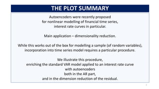
The document explores the use of autoencoders for nonlinear modeling of financial time series, particularly interest rate curves, with an emphasis on dimensionality reduction. It presents a methodology to enhance traditional VAR models by integrating autoencoders and discusses the challenges related to distinguishing between sample and time series data. The analysis includes comparisons of various model types and their effectiveness, revealing insights into residual behaviors and correlations in the context of interest rate swaps from 2010 to 2023.

1. AEN-VAR-AEN
time series modelling with autoencoders
preliminary results
Andrey Chirikhin
andrey.chirikhin@barclays.com
The 19th WBS Quantitative Finance Conference
28 September 2023
Vacencia

2. Autoencoders were recently proposed
for nonlinear modelling of financial time series,
interest rate curves in particular.
Main application – dimensionality reduction.
While this works out of the box for modelling a sample (of random variables),
incorporation into time series model requires a particular procedure.
We illustrate this procedure,
enriching the standard VAR model applied to an interest rate curve
with autoencoders
both in the AR part,
and in the dimension reduction of the residual.
THE PLOT SUMMARY
2

3. THE SHOOTING SCRIPT
3
The prologue
Samples vs time series
The sacred purpose of TSA
Act 2
AR VAR NVAR
Act 1
Is(n’t) AR(1) enough?
Act 3
The residuals: PCA vs AEN
aka The tail of two methods for the dimensionality reduction not to be afraid of.

4. THE SHOOTING SCRIPT
4
The prologue
Samples vs time series
The sacred purpose of TSA

5. TIME SERIES VS SAMPLES
5
Consider a series of observations of a (stochastic) vector variable.
Otherwise,
it is a time series (TS).
Order matters and
the model may have to reproduce
certain time-dependent features
of the original TS.
It is a sample,
if the order of observations can be shuffled.
Only values matter, but not the order.
Typically, a (stationary) distribution
Is being estimated, or, more generally
a function is being fitted (ML)
Unless the data is obtained from an “in vitru” controlled experiment,
or the problem clearly does not have time dimension,
to consider observations a sample and not a time series is… risky.
Depending on the problem being solved,
same observations can be considered upfront
a sample or a time series, the former usually requiring that sample is, actually, a stationary TS
but changing your view in the middle of analysis can yield equally unpredictable outcome.

6. SEPARATING CORRELATION AND CAUSATION
6
One can define time series modelling as
extracting the causation model
until residuals become at least serially independent.
Why iid residuals?
1. Historical simulation or
similar sample-based
nonparametric methods
2. Parametric estimation of
the model for
the 𝜖 scalar or vector,
usually via Likelihood,
so factorization is useful.
3. Target for the
non-linear AR estimation
using scheme similar to (2).
causation correlation
ARMA(N,M) 𝑥𝑛 = 𝑎0 + ෍
𝑖=1
𝑁
𝑎𝑖𝑥𝑛−𝑖 + ෍
𝑗=1
𝑀
𝑏𝑗𝜖𝑛−𝑗 𝑥𝑛, 𝜖𝑛, 𝑎𝑖, 𝑏𝑗 ∈ 𝑅
VARMA(N,M) 𝑋𝑛 = 𝐴0 + ෍
𝑖=1
𝑁
𝐴𝑖𝑋𝑛−𝑖 + ෍
𝑗=1
𝑀
𝐵𝑗Ε𝑛−𝑗
𝑋𝑛, Ε𝑛, 𝐴0, ∈ 𝑅𝑛
𝐴𝑖, 𝐵𝑗 ∈ 𝑅𝑛×𝑛
NVARMA(N,M) 𝑋𝑛 = Α 𝑋𝑛−1, … , 𝑋𝑛−𝑁 + Β Ε𝑛−1, … , Ε𝑛−𝑀
𝑋𝑛, Ε𝑛 ∈ 𝑅𝑛
Α: 𝑅𝑛×𝑁
→ 𝑅𝑛
Β: 𝑅𝑛×𝑀
→ 𝑅𝑛
𝝐𝒏, 𝚬𝒏 are assumed iid, no serial dependency

7. AEN GENEALOGY
7
This is the first time AENs are used in the TSA setting, both for AR and correlation dimensionality reduction
Author Year Domain Image Autoencoder
A. Kondratiev 2018 𝑠𝑖(𝜏) 𝑠𝑖(𝜏) AEN
A. Sokol 2022 𝑠𝑖(𝜏) 𝑠𝑖(𝜏) VAE
J. Andreasen 2023 𝑠𝑖(𝜏) 𝐷𝐹𝑖(𝜏) AEN
A. Chirikhin 2023 𝑠𝑖(𝜏) 𝑠𝑖+1(𝜏) AEN
𝜖𝑖(𝜏) 𝜖𝑖(𝜏) AEN

8. ACT 1
8
Is(n’t) AR(1) enough?

9. THE DATASET
9
Motivated by the one used by Kondratiev/Sokol/Andreasen
“Old style” Libor IRS swaps, USSWAPxx Curncy
1y, 2y, 3y, 5y, 10y, 7y, 15y, 20y, 30y, 50y (10 points)
01/01/2010-01/01/2023
weekly observations
679 points in total

10. NI QUESTION: WHAT DOES IT LOOK LIKE???
10

11. SELECTED TENORS AND DATES
11
Level, slope and curvature are present,… and something else?
Mind the inversion!

12. NONSTATIONARY SAMPLE…
12
…results in nonstationary model parameters, if effort is made to check for that.
One can be tempted to invent a trading strategy around this!

13. OVERLAPPING SERIES DOES NOT HELP
13
Rolling pairwise correlations are entirely spurious
Solution?
1. Estimate AR(1) per tenor
Δ𝑠𝑛 = 𝑎0 + 𝑏𝑠𝑛 + 𝜖𝑛 ⟺
𝑠𝑛+1 = 𝑎0 + 𝑎1𝑠𝑛 + 𝜖𝑛
2. Extract residuals
𝜖𝑛 = 𝑠𝑛+1 − 𝑎0 − 𝑎1𝑠𝑛
3. Study their correlation
Note
Usually, 𝑎1 ≈ 1, hence
𝜖𝑛 ≈ 𝑠𝑛+1 − 𝑠𝑛 − 𝑎0 =
Δ𝑠𝑛 −𝑎0.
Can study correlations of a
difference, without
estimating the model

14. Observable:
Stock price time series 𝑋𝑖
Stock returns:
Δ𝑋𝑖
𝑋𝑖
= 𝑟𝑖
𝑟𝑖+1 = A + B × 𝑟𝑖 +𝜖𝑖,
For stocks B ≈ 0,
𝑟𝑖+1 is stationary, white noise.
INTUITION FOR AR(1), AND AR IN GENERAL
14
Despite IRS spreads (or any other yield-like quantities) has the unit of returns,
they are not compatible with equity returns.
Yields are rather like equities themselves.
Nobody correlates equities, only equity returns.
Observable:
Bond yield time series 𝑦𝑖
Bond returns:
Δ𝐵𝑖
𝐵𝑖
= Δ𝑦𝑖 × 𝐷𝑢𝑟𝑎𝑡𝑖𝑜𝑛
Δ𝑦𝑖 = 𝑎 𝑏 − 𝑦𝑖 𝛿𝑡 + 𝜂𝑖 (“Vasicek”)
𝑦𝑖+1 = P + 𝑄 × 𝑦𝑖 +𝜂𝑖,
For bonds: 𝑄 ≲ 1,
𝑦𝑖+1 is stationary, 𝑚𝑒𝑎𝑛 𝑟𝑒𝑣𝑒𝑟𝑖𝑛𝑔
AR(1) process in both cases. Estimated by linear regression.
But because B ≈ 0, while 𝑄 ≲ 1, 𝑟𝑖+1~ Δ𝑦𝑖, and not 𝑟𝑖+1~ 𝑦𝑖+1, also as revealed by the returns equation.
Yields is, merely a price “adjusted for time to maturity: 𝑦(𝑡) = −ln 𝐵(𝑡)/(𝑇 − 𝑡) , so behaves like a price.

15. RESIDUALS’ CORRELATIONS
15
Sadly, no correlation trading system…
Still, why the spike?

16. RESIDUALS’ CORRELATIONS VS RATES
16
Covid
But are the
residuals i.i.d?
Have they
become a sample?

17. RESIDUALS’ AUTOCORRELATIONS
17
Look a bit volatile
Mind the
autocorrelation
confidence
interval:
±
𝒁𝜶/𝟐
𝑺𝒂𝒎𝒑𝒍𝒆𝑺𝒊𝒛𝒆
= ±
𝟏. 𝟗𝟔
𝟓𝟐
= ±0.027

18. RESIDUALS’ AUTOCORRELATION
18
i.i.d enough already
Why
1-year point
is always
odd?

19. 1-YEAR RUNNING SLOPES
19
USSWAP1 is nonstationary

20. ACT 1, SUMMARY
20
Most series are stationary.
After switch to residuals, correlations are much more stable.
Residual autocorrelations close to 0, so it is a sample.
Model seems to be well identified.
We could have stopped here.
Do we even need to further understand residual correlations?
This is parametric vs non-parametric question again, in a way.
More relevant for historical estimates of correlations where necessary.

21. ACT 2
21
AR VAR NVAR
For the full sample of 10 tenors:
Estimate AR, VAR and NVAR
…using different NN topologies,
compare AR functions,
residual autocorrelations,
pairwise correlations and PCAs.

22. THE MODELS
22
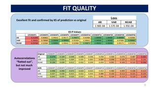
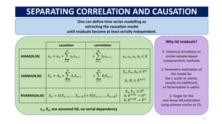
3 types of lag-1 models were estimated
Model Dynamics Method
AR(1)
Per tenor
𝑥𝑛 = 𝑎0 + 𝑎1𝑥𝑛−1 + 𝜖𝑛 tsa.ar_model.AutoReg
VAR(1) 𝑋𝑛 = 𝐴0 + 𝐴1𝑋𝑛−1 + Ε𝑛 tsa.VAR
NVAR(1) 𝑋𝑛 = Α(𝑋𝑛−1) + Ε𝑛 sklearn.neural_network
.MLPRegressor
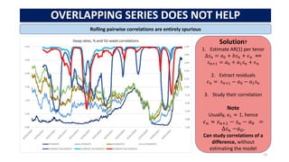
Different topologies for operator Α in NVAR(1,1) were tried,
and the one with the lowest loss chosen: [20], which was superior to [10,2,10] AEN.
RELU activation and LBGFS yield best results, probably due to the relatively small sample size,
To find a NVAR “equivalent” matrix to the VAR’s 𝑨𝟏, the identity matrix was predicted with fitted NVAR.

23. AR MATRICES
23
AR
1.0094
1.0061
1.0025
0.9959
0.9915
0.9894
0.9892
0.9892
0.9891
0.9876
VAR diff
18.34 2.80
- 2.53
- 1.49
- 1.95
- 2.10
- 2.08
- 1.93
- 1.65
- 1.65
- 17.33 2.80
- 2.53
- 1.49
- 1.95
- 2.10
- 2.08
- 1.93
- 1.65
- 1.65
-
2.22 5.78 1.62 0.53 1.13 1.30 1.21 1.05 0.82 1.10 2.22 4.77 1.62 0.53 1.13 1.30 1.21 1.05 0.82 1.10
0.74
- 0.50
- 1.71 0.34 0.46
- 0.66
- 0.58
- 0.46
- 0.32
- 0.87
- 0.74
- 0.50
- 0.71 0.34 0.46
- 0.66
- 0.58
- 0.46
- 0.32
- 0.87
-
0.41 0.17
- 0.02
- 0.84 0.20 0.33 0.52 0.52 0.57 1.25 0.41 0.17
- 0.02
- 0.16
- 0.20 0.33 0.52 0.52 0.57 1.25
1.13
- 0.03 0.12 0.38 0.73 0.30
- 0.76
- 0.83
- 1.03
- 1.30
- 1.13
- 0.03 0.12 0.38 0.27
- 0.30
- 0.76
- 0.83
- 1.03
- 1.30
-
1.74 0.57 0.38 0.31 0.56 1.43 0.66 0.61 0.78 0.97 1.74 0.57 0.38 0.31 0.56 0.44 0.66 0.61 0.78 0.97
2.07
- 1.92
- 1.85
- 1.52
- 1.08
- 0.47
- 1.04 0.23 0.29 0.52 2.07
- 1.92
- 1.85
- 1.52
- 1.08
- 0.47
- 0.05 0.23 0.29 0.52
2.20 1.81 1.63 1.30 0.87 0.50 0.33 1.31 0.00
- 2.22
- 2.20 1.81 1.63 1.30 0.87 0.50 0.33 0.32 0.00
- 2.22
-
1.25
- 0.01
- 0.31 0.29 0.30 0.12 0.36
- 0.40
- 1.76 3.97 1.25
- 0.01
- 0.31 0.29 0.30 0.12 0.36
- 0.40
- 0.77 3.97
1.24
- 1.97
- 1.94
- 1.66
- 1.39
- 0.90
- 0.24
- 0.01 0.53 4.09 1.24
- 1.97
- 1.94
- 1.66
- 1.39
- 0.90
- 0.24
- 0.01 0.53 3.10
NVAR diff
0.45 0.11 0.03 0.09
- 0.20 0.13 0.09
- 0.11 0.10 0.17 0.56
- 0.11 0.03 0.09
- 0.20 0.13 0.09
- 0.11 0.10 0.17
0.22 1.17 0.69 0.05
- 0.13 0.37 0.10
- 0.43 0.24 0.56 0.22 0.17 0.69 0.05
- 0.13 0.37 0.10
- 0.43 0.24 0.56
0.01 0.42 0.10 0.36 0.01
- 0.60 0.03 0.30 0.03 0.16 0.01 0.42 0.91
- 0.36 0.01
- 0.60 0.03 0.30 0.03 0.16
0.47 0.12 0.12
- 0.06 0.16 0.36 0.20
- 0.03
- 0.05
- 0.12 0.47 0.12 0.12
- 0.94
- 0.16 0.36 0.20
- 0.03
- 0.05
- 0.12
0.12
- 0.26 0.20 0.24 0.39 0.51 0.12 0.31 0.40 0.12 0.12
- 0.26 0.20 0.24 0.60
- 0.51 0.12 0.31 0.40 0.12
0.37 0.36 0.04
- 0.00 0.10 0.51 0.00 0.20 0.23 0.14 0.37 0.36 0.04
- 0.00 0.10 0.48
- 0.00 0.20 0.23 0.14
0.24 0.25 0.00
- 0.04 0.45 0.40 0.24 0.34 0.09 0.02 0.24 0.25 0.00
- 0.04 0.45 0.40 0.75
- 0.34 0.09 0.02
0.13 0.17 0.23
- 0.17 0.21 0.72 0.36 0.50 0.34 0.11 0.13 0.17 0.23
- 0.17 0.21 0.72 0.36 0.49
- 0.34 0.11
0.10
- 0.50 0.12 0.08 0.05 0.16 0.15 0.28 0.37 0.49 0.10
- 0.50 0.12 0.08 0.05 0.16 0.15 0.28 0.61
- 0.49
0.00
- 0.07
- 0.02 0.03 0.08 0.05 0.12
- 0.01 0.28 0.76 0.00
- 0.07
- 0.02 0.03 0.08 0.05 0.12
- 0.01 0.28 0.23
-
AR is best
revealing several non-stationarities
VAR is spurious
possibly “implementation feature”
NVAR needs more detailed analysis,
but definitely does something different

24. RESIDUAL AUTOCORRELATIONS
24
VAR and NVAR look very similar, improving on the worst case of 1Y.
Given the sample size of 678, the confidence interval is
(-0.0725, 0.0752).
More than half of the values too high.
Higher AR order is necessary.
USSWAP1 USSWAP2 USSWAP3 USSWAP5 USSWAP7 USSWAP10 USSWAP15 USSWAP20 USSWAP30 USSWAP50
AR 0.27 0.10 0.05 0.01
- 0.04
- 0.06
- 0.07
- 0.08
- 0.09
- 0.16
-
VAR 0.12 0.03 0.01 0.03
- 0.06
- 0.08
- 0.10
- 0.10
- 0.11
- 0.14
-
NVAR 0.14 0.04 0.01 0.03
- 0.04
- 0.06
- 0.09
- 0.10
- 0.12
- 0.16
-

25. AR
1.00 0.89 0.77 0.62 0.55 0.48 0.42 0.39 0.35 0.32
0.89 1.00 0.96 0.86 0.78 0.70 0.62 0.58 0.52 0.49
0.77 0.96 1.00 0.95 0.89 0.81 0.74 0.69 0.63 0.59
0.62 0.86 0.95 1.00 0.98 0.93 0.87 0.83 0.78 0.73
0.55 0.78 0.89 0.98 1.00 0.98 0.95 0.91 0.87 0.81
0.48 0.70 0.81 0.93 0.98 1.00 0.99 0.97 0.94 0.87
0.42 0.62 0.74 0.87 0.95 0.99 1.00 1.00 0.98 0.91
0.39 0.58 0.69 0.83 0.91 0.97 1.00 1.00 0.99 0.92
0.35 0.52 0.63 0.78 0.87 0.94 0.98 0.99 1.00 0.93
0.32 0.49 0.59 0.73 0.81 0.87 0.91 0.92 0.93 1.00
VAR diff
1.00 0.90 0.78 0.63 0.55 0.47 0.41 0.37 0.33 0.31 0E+00 7E-03 1E-02 4E-03 -4E-03 -1E-02 -2E-02 -2E-02 -2E-02 -1E-02
0.90 1.00 0.97 0.86 0.78 0.69 0.62 0.57 0.52 0.48 7E-03 0E+00 7E-04 -3E-04 -3E-03 -5E-03 -6E-03 -5E-03 -4E-03 -7E-03
0.78 0.97 1.00 0.95 0.89 0.81 0.74 0.69 0.63 0.59 1E-02 7E-04 0E+00 3E-04 -1E-03 -2E-03 -2E-03 -5E-04 8E-04 -2E-03
0.63 0.86 0.95 1.00 0.98 0.93 0.87 0.84 0.78 0.73 4E-03 -3E-04 3E-04 0E+00 5E-04 6E-04 1E-03 3E-03 4E-03 4E-03
0.55 0.78 0.89 0.98 1.00 0.98 0.95 0.92 0.87 0.82 -4E-03 -3E-03 -1E-03 5E-04 0E+00 1E-04 9E-04 2E-03 3E-03 7E-03
0.47 0.69 0.81 0.93 0.98 1.00 0.99 0.97 0.94 0.88 -1E-02 -5E-03 -2E-03 6E-04 1E-04 0E+00 6E-04 1E-03 2E-03 1E-02
0.41 0.62 0.74 0.87 0.95 0.99 1.00 1.00 0.98 0.92 -2E-02 -6E-03 -2E-03 1E-03 9E-04 6E-04 0E+00 2E-04 7E-04 1E-02
0.37 0.57 0.69 0.84 0.92 0.97 1.00 1.00 0.99 0.94 -2E-02 -5E-03 -5E-04 3E-03 2E-03 1E-03 2E-04 0E+00 2E-04 2E-02
0.33 0.52 0.63 0.78 0.87 0.94 0.98 0.99 1.00 0.95 -2E-02 -4E-03 8E-04 4E-03 3E-03 2E-03 7E-04 2E-04 0E+00 2E-02
0.31 0.48 0.59 0.73 0.82 0.88 0.92 0.94 0.95 1.00 -1E-02 -7E-03 -2E-03 4E-03 7E-03 1E-02 1E-02 2E-02 2E-02 0E+00
NVAR diff
1.00 0.89 0.78 0.63 0.54 0.46 0.40 0.38 0.33 0.30 0.0E+00 -3.6E-03 6.0E-03 4.0E-03 -8.8E-03 -1.6E-02 -2.1E-02 -1.4E-02 -1.6E-02 -2.2E-02
0.89 1.00 0.95 0.84 0.77 0.69 0.61 0.56 0.51 0.47 -3.6E-03 0.0E+00 -1.4E-02 -1.2E-02 -4.7E-03 -6.3E-03 -1.5E-02 -1.3E-02 -1.2E-02 -1.6E-02
0.78 0.95 1.00 0.95 0.87 0.79 0.72 0.68 0.63 0.58 6.0E-03 -1.4E-02 0.0E+00 -7.6E-04 -1.8E-02 -2.0E-02 -2.0E-02 -8.2E-03 -7.6E-04 -1.1E-02
0.63 0.84 0.95 1.00 0.97 0.92 0.86 0.83 0.78 0.72 4.0E-03 -1.2E-02 -7.6E-04 0.0E+00 -1.5E-02 -1.6E-02 -1.4E-02 -4.3E-03 2.1E-03 -4.3E-03
0.54 0.77 0.87 0.97 1.00 0.98 0.94 0.90 0.86 0.80 -8.8E-03 -4.7E-03 -1.8E-02 -1.5E-02 0.0E+00 -2.9E-03 -7.9E-03 -1.1E-02 -1.0E-02 -7.1E-03
0.46 0.69 0.79 0.92 0.98 1.00 0.98 0.96 0.93 0.87 -1.6E-02 -6.3E-03 -2.0E-02 -1.6E-02 -2.9E-03 0.0E+00 -4.1E-03 -8.8E-03 -8.2E-03 4.4E-04
0.40 0.61 0.72 0.86 0.94 0.98 1.00 0.99 0.97 0.91 -2.1E-02 -1.5E-02 -2.0E-02 -1.4E-02 -7.9E-03 -4.1E-03 0.0E+00 -3.0E-03 -6.6E-03 -5.8E-04
0.38 0.56 0.68 0.83 0.90 0.96 0.99 1.00 0.99 0.92 -1.4E-02 -1.3E-02 -8.2E-03 -4.3E-03 -1.1E-02 -8.8E-03 -3.0E-03 0.0E+00 -3.5E-03 -1.9E-03
0.33 0.51 0.63 0.78 0.86 0.93 0.97 0.99 1.00 0.94 -1.6E-02 -1.2E-02 -7.6E-04 2.1E-03 -1.0E-02 -8.2E-03 -6.6E-03 -3.5E-03 0.0E+00 1.2E-02
0.30 0.47 0.58 0.72 0.80 0.87 0.91 0.92 0.94 1.00 -2.2E-02 -1.6E-02 -1.1E-02 -4.3E-03 -7.1E-03 4.4E-04 -5.8E-04 -1.9E-03 1.2E-02 0.0E+00
RESIDUAL CORRELATIONS
25
Nearly identical
Slightly larger differences for NVAR

26. PCA
26
PCA nearly identical for the 3 models

27. ACT 2, SUMMARY
27
As expected, AR already nearly good enough,
higher AR order necessary for the extreme tenors.
VAR highlights multicollinearity.
NVAR requires fine tuning.

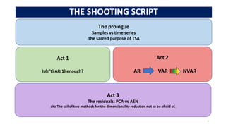
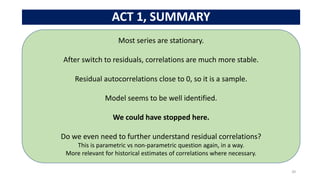
28. ACT 3
28
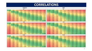
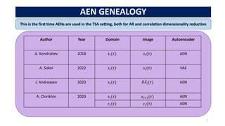
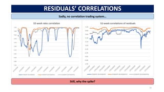
The residuals: PCA vs AEN
1. Fit a [10,2,10] autoencoder
…for residuals of estimated AR, VAR and NVAR models.
2. Predict residuals.
3. Compare their correlation matrices to the original ones.
4. Test closeness of the predicted residuals to the original residuals
… using Kolmogorov-Smirnov test
(which is justified, if residuals are not autocorrelated,
hence samples).

29. FIT QUALITY
29
Original USSWAP1 USSWAP2 USSWAP3 USSWAP5 USSWAP7 USSWAP10 USSWAP15 USSWAP20 USSWAP30 USSWAP50
AR 0.274 0.104 0.048 0.008
- 0.036
- 0.058
- 0.068
- 0.076
- 0.087
- 0.162
-
VAR 0.123 0.034 0.009 0.035
- 0.063
- 0.084
- 0.098
- 0.105
- 0.114
- 0.135
-
NVAR 0.136 0.039 0.012 0.032
- 0.039
- 0.059
- 0.091
- 0.103
- 0.115
- 0.156
-
AEN USSWAP1 USSWAP2 USSWAP3 USSWAP5 USSWAP7 USSWAP10 USSWAP15 USSWAP20 USSWAP30 USSWAP50
AR 0.098 0.090 0.072 0.024 0.015
- 0.053
- 0.080
- 0.093
- 0.106
- 0.113
-
VAR 0.037 0.030 0.015 0.022
- 0.054
- 0.080
- 0.102
- 0.112
- 0.121
- 0.125
-
NVAR 0.043 0.035 0.020 0.019
- 0.051
- 0.081
- 0.104
- 0.113
- 0.123
- 0.128
-
Autocorrelations
“flatted out”,
but not much
improved
Excellent fit and confirmed by KS of prediction vs original
Loss
AR VAR NVAR
1.90E-04 1.57E-04 1.95E-04
KS P-Values
USSWAP1 USSWAP2 USSWAP3 USSWAP5 USSWAP7 USSWAP10 USSWAP15 USSWAP20 USSWAP30 USSWAP50
AR 0.21204 0.86802 0.99642 0.99171 0.99873 0.92984 1.00000 1.00000 0.99999 0.92984
VAR 0.39830 0.78969 0.99999 0.99993 0.95304 0.99642 0.99999 1.00000 0.97084 0.99965
NVAR 0.23744 0.92984 0.99993 0.99642 0.92984 0.99873 0.99993 0.99999 0.99171 0.95304

30. CORRELATIONS
30
Original AEN
AR AR
1.00 0.89 0.77 0.62 0.55 0.48 0.42 0.39 0.35 0.32 1.00 0.99 0.95 0.84 0.73 0.61 0.50 0.45 0.37 0.33
0.89 1.00 0.96 0.86 0.78 0.70 0.62 0.58 0.52 0.49 0.99 1.00 0.99 0.92 0.83 0.73 0.64 0.59 0.52 0.48
0.77 0.96 1.00 0.95 0.89 0.81 0.74 0.69 0.63 0.59 0.95 0.99 1.00 0.97 0.91 0.83 0.75 0.70 0.65 0.60
0.62 0.86 0.95 1.00 0.98 0.93 0.87 0.83 0.78 0.73 0.84 0.92 0.97 1.00 0.98 0.94 0.89 0.86 0.82 0.79
0.55 0.78 0.89 0.98 1.00 0.98 0.95 0.91 0.87 0.81 0.73 0.83 0.91 0.98 1.00 0.99 0.96 0.94 0.91 0.88
0.48 0.70 0.81 0.93 0.98 1.00 0.99 0.97 0.94 0.87 0.61 0.73 0.83 0.94 0.99 1.00 0.99 0.98 0.96 0.95
0.42 0.62 0.74 0.87 0.95 0.99 1.00 1.00 0.98 0.91 0.50 0.64 0.75 0.89 0.96 0.99 1.00 1.00 0.99 0.98
0.39 0.58 0.69 0.83 0.91 0.97 1.00 1.00 0.99 0.92 0.45 0.59 0.70 0.86 0.94 0.98 1.00 1.00 1.00 0.99
0.35 0.52 0.63 0.78 0.87 0.94 0.98 0.99 1.00 0.93 0.37 0.52 0.65 0.82 0.91 0.96 0.99 1.00 1.00 1.00
0.32 0.49 0.59 0.73 0.81 0.87 0.91 0.92 0.93 1.00 0.33 0.48 0.60 0.79 0.88 0.95 0.98 0.99 1.00 1.00
VAR VAR
1.00 0.90 0.78 0.63 0.55 0.47 0.41 0.37 0.33 0.31 1.00 0.98 0.94 0.82 0.70 0.59 0.47 0.40 0.33 0.30
0.90 1.00 0.97 0.86 0.78 0.69 0.62 0.57 0.52 0.48 0.98 1.00 0.99 0.92 0.83 0.73 0.64 0.58 0.51 0.48
0.78 0.97 1.00 0.95 0.89 0.81 0.74 0.69 0.63 0.59 0.94 0.99 1.00 0.97 0.91 0.83 0.75 0.69 0.64 0.61
0.63 0.86 0.95 1.00 0.98 0.93 0.87 0.84 0.78 0.73 0.82 0.92 0.97 1.00 0.98 0.94 0.89 0.85 0.81 0.79
0.55 0.78 0.89 0.98 1.00 0.98 0.95 0.92 0.87 0.82 0.70 0.83 0.91 0.98 1.00 0.99 0.96 0.93 0.90 0.89
0.47 0.69 0.81 0.93 0.98 1.00 0.99 0.97 0.94 0.88 0.59 0.73 0.83 0.94 0.99 1.00 0.99 0.98 0.96 0.95
0.41 0.62 0.74 0.87 0.95 0.99 1.00 1.00 0.98 0.92 0.47 0.64 0.75 0.89 0.96 0.99 1.00 1.00 0.99 0.98
0.37 0.57 0.69 0.84 0.92 0.97 1.00 1.00 0.99 0.94 0.40 0.58 0.69 0.85 0.93 0.98 1.00 1.00 1.00 0.99
0.33 0.52 0.63 0.78 0.87 0.94 0.98 0.99 1.00 0.95 0.33 0.51 0.64 0.81 0.90 0.96 0.99 1.00 1.00 1.00
0.31 0.48 0.59 0.73 0.82 0.88 0.92 0.94 0.95 1.00 0.30 0.48 0.61 0.79 0.89 0.95 0.98 0.99 1.00 1.00
NVAR NVAR
1.00 0.89 0.78 0.63 0.54 0.46 0.40 0.38 0.33 0.30 1.00 0.98 0.94 0.82 0.71 0.59 0.47 0.41 0.34 0.29
0.89 1.00 0.95 0.84 0.77 0.69 0.61 0.56 0.51 0.47 0.98 1.00 0.99 0.92 0.84 0.73 0.63 0.58 0.51 0.47
0.78 0.95 1.00 0.95 0.87 0.79 0.72 0.68 0.63 0.58 0.94 0.99 1.00 0.97 0.91 0.83 0.74 0.70 0.64 0.60
0.63 0.84 0.95 1.00 0.97 0.92 0.86 0.83 0.78 0.72 0.82 0.92 0.97 1.00 0.98 0.94 0.89 0.86 0.81 0.78
0.54 0.77 0.87 0.97 1.00 0.98 0.94 0.90 0.86 0.80 0.71 0.84 0.91 0.98 1.00 0.99 0.95 0.93 0.90 0.88
0.46 0.69 0.79 0.92 0.98 1.00 0.98 0.96 0.93 0.87 0.59 0.73 0.83 0.94 0.99 1.00 0.99 0.98 0.96 0.95
0.40 0.61 0.72 0.86 0.94 0.98 1.00 0.99 0.97 0.91 0.47 0.63 0.74 0.89 0.95 0.99 1.00 1.00 0.99 0.98
0.38 0.56 0.68 0.83 0.90 0.96 0.99 1.00 0.99 0.92 0.41 0.58 0.70 0.86 0.93 0.98 1.00 1.00 1.00 0.99
0.33 0.51 0.63 0.78 0.86 0.93 0.97 0.99 1.00 0.94 0.34 0.51 0.64 0.81 0.90 0.96 0.99 1.00 1.00 1.00
0.30 0.47 0.58 0.72 0.80 0.87 0.91 0.92 0.94 1.00 0.29 0.47 0.60 0.78 0.88 0.95 0.98 0.99 1.00 1.00

31. Straightforward VAR does not improve on AR
over the long-term sample.
Rolling analysis is necessary,
with smaller time step.
Non-linear AR kernel needs fine-tuning.
Autoencoding residuals converges better
than in the previous experiments with spreads,
but does not have material effect.
VAR worked much better for credit and vols,
so AEN should be tried there.
ACT 3 AND FINAL FINDINGS
31