Download to read offline


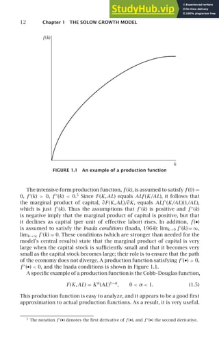
![8 Chapter 1 THE SOLOW GROWTH MODEL
means that the overall dispersion of average incomes across different parts
of the world must have been much smaller than it is today (Pritchett, 1997).
Over the past few decades, however, there has been no strong tendency
either toward continued divergence or toward convergence.
The implications of the vast differences in standards of living over time
and across countries for human welfare are enormous. The differences are
associated with large differences in nutrition, literacy, infant mortality, life
expectancy, and other direct measures of well-being. And the welfare con-
sequences of long-run growth swamp any possible effects of the short-run
fluctuations that macroeconomics traditionally focuses on. During an av-
erage recession in the United States, for example, real income per person
falls by a few percent relative to its usual path. In contrast, the productivity
growth slowdown reduced real income per person in the United States by
about 25 percent relative to what it otherwise would have been. Other exam-
ples are even more startling. If real income per person in the Philippines con-
tinues to grow at its average rate for the period 1960–2001 of 1.5 percent, it
will take 150 years for it to reach the current U.S. level. If it achieves 3 per-
cent growth, the time will be reduced to 75 years. And if it achieves 5 percent
growth, as the NICs have done, the process will take only 45 years. To quote
Robert Lucas (1988), “Once one starts to think about [economic growth], it
is hard to think about anything else.”
The first four chapters of this book are therefore devoted to economic
growth. We will investigate several models of growth. Although we will
examine the models’ mechanics in considerable detail, our goal is to learn
what insights they offer concerning worldwide growth and income differ-
ences across countries. Indeed, the ultimate objective of research on eco-
nomic growth is to determine whether there are possibilities for raising
overall growth or bringing standards of living in poor countries closer to
those in the world leaders.
This chapter focuses on the model that economists have traditionally
used to study these issues, the Solow growth model.3
The Solow model is
the starting point for almost all analyses of growth. Even models that depart
fundamentally from Solow’s are often best understood through comparison
with the Solow model. Thus understanding the model is essential to under-
standing theories of growth.
The principal conclusion of the Solow model is that the accumulation
of physical capital cannot account for either the vast growth over time in
output per person or the vast geographic differences in output per per-
son. Specifically, suppose that capital accumulation affects output through
the conventional channel that capital makes a direct contribution to pro-
duction, for which it is paid its marginal product. Then the Solow model
3
The Solow model (which is sometimes known as the Solow–Swan model) was developed
by Robert Solow (Solow, 1956) and T. W. Swan (Swan, 1956).](https://image.slidesharecdn.com/advanced-macroeconomics-230806183016-1212def2/85/Advanced-Macroeconomics-30-320.jpg)

![14 Chapter 1 THE SOLOW GROWTH MODEL
The growth rate of a variable refers to its proportional rate of change.
That is, the growth rate of X refers to the quantity ˙
X (t)/X(t). Thus equa-
tion (1.8) implies that the growth rate of L is constant and equal to n, and
(1.9) implies that A’s growth rate is constant and equal to g.
A key fact about growth rates is that the growth rate of a variable equals
the rate of change of its natural log. That is, Ẋ (t)/X(t) equals d ln X(t)/dt. To
see this, note that since ln X is a function of X and X is a function of t, we
can use the chain rule to write
d ln X(t)
dt
=
d ln X(t)
dX(t)
dX(t)
dt
=
1
X(t)
Ẋ (t).
(1.10)
Applying the result that a variable’s growth rate equals the rate of change
of its log to (1.8) and (1.9) tells us that the rates of change of the logs of L
and A are constant and that they equal n and g, respectively. Thus,
ln L(t) = [ln L(0)] + nt, (1.11)
ln A(t) = [ln A(0)] + gt, (1.12)
where L(0) and A(0) are the values of L and A at time 0. Exponentiating both
sides of these equations gives us
L(t) = L(0)ent
, (1.13)
A(t) = A(0)egt
. (1.14)
Thus, our assumption is that L and A each grow exponentially.8
Output is divided between consumption and investment. The fraction
of output devoted to investment, s, is exogenous and constant. One unit of
output devoted to investment yields one unit of new capital. In addition,
existing capital depreciates at rate δ. Thus
K̇(t) = sY(t) − δK(t). (1.15)
Although no restrictions are placed on n, g, and δ individually, their sum is
assumed to be positive. This completes the description of the model.
Since this is the first model (of many!) we will encounter, this is a good
place for a general comment about modeling. The Solow model is grossly
simplified in a host of ways. To give just a few examples, there is only a
single good; government is absent; fluctuations in employment are ignored;
production is described by an aggregate production function with just three
inputs; and the rates of saving, depreciation, population growth, and tech-
nological progress are constant. It is natural to think of these features of
the model as defects: the model omits many obvious features of the world,
8
See Problems 1.1 and 1.2 for more on basic properties of growth rates.](https://image.slidesharecdn.com/advanced-macroeconomics-230806183016-1212def2/85/Advanced-Macroeconomics-36-320.jpg)
![1.3 The Dynamics of the Model 15
and surely some of those features are important to growth. But the purpose
of a model is not to be realistic. After all, we already possess a model that
is completely realistic—the world itself. The problem with that “model” is
that it is too complicated to understand. A model’s purpose is to provide
insights about particular features of the world. If a simplifying assump-
tion causes a model to give incorrect answers to the questions it is being
used to address, then that lack of realism may be a defect. (Even then, the
simplification—by showing clearly the consequences of those features of
the world in an idealized setting—may be a useful reference point.) If the
simplification does not cause the model to provide incorrect answers to the
questions it is being used to address, however, then the lack of realism is
a virtue: by isolating the effect of interest more clearly, the simplification
makes it easier to understand.
1.3 The Dynamics of the Model
We want to determine the behavior of the economy we have just described.
The evolution of two of the three inputs into production, labor and knowl-
edge, is exogenous. Thus to characterize the behavior of the economy, we
must analyze the behavior of the third input, capital.
The Dynamics of k
Because the economy may be growing over time, it turns out to be much
easier to focus on the capital stock per unit of effective labor, k, than on the
unadjusted capital stock, K. Since k = K/AL, we can use the chain rule to
find
˙
k(t) =
K̇(t)
A(t)L(t)
−
K(t)
[A(t)L(t)]2
[A(t)L̇(t) + L(t)Ȧ(t)]
=
K̇(t)
A(t)L(t)
−
K(t)
A(t)L(t)
L̇(t)
L(t)
−
K(t)
A(t)L(t)
Ȧ(t)
A(t)
.
(1.16)
K/AL is simply k. From (1.8) and (1.9), L̇/L and Ȧ/A are n and g, respectively.
K̇ is given by (1.15). Substituting these facts into (1.16) yields
˙
k(t) =
sY(t) − δK(t)
A(t)L(t)
− k(t)n − k(t)g
= s
Y(t)
A(t)L(t)
− δk(t) − nk(t) − gk(t).
(1.17)](https://image.slidesharecdn.com/advanced-macroeconomics-230806183016-1212def2/85/Advanced-Macroeconomics-37-320.jpg)
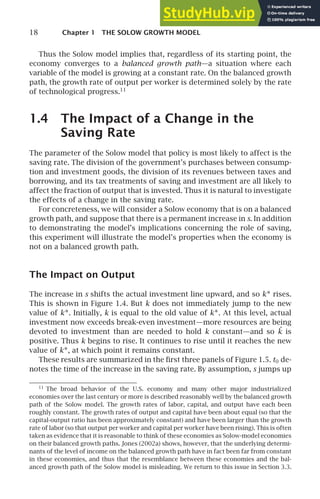
![1.4 The Impact of a Change in the Saving Rate 21
Solow model only changes in the rate of technological progress have growth
effects; all other changes have only level effects.
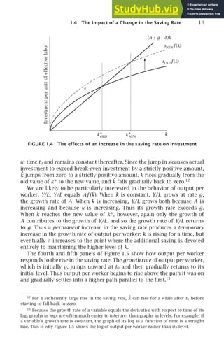
The Impact on Consumption
If we were to introduce households into the model, their welfare would de-
pend not on output but on consumption: investment is simply an input into
production in the future. Thus for many purposes we are likely to be more
interested in the behavior of consumption than in the behavior of output.
Consumption per unit of effective labor equals output per unit of effec-
tive labor, f (k), times the fraction of that output that is consumed, 1 − s.
Thus, since s changes discontinuously at t0 and k does not, initially con-
sumption per unit of effective labor jumps downward. Consumption then
rises gradually as k rises and s remains at its higher level. This is shown in
the last panel of Figure 1.5.
Whether consumption eventually exceeds its level before the rise in s is
not immediately clear. Let c∗ denote consumption per unit of effective labor
on the balanced growth path. c∗ equals output per unit of effective labor,
f (k∗), minus investment per unit of effective labor, sf (k∗). On the balanced
growth path, actual investment equals break-even investment, (n + g+δ)k∗.
Thus,
c∗ = f (k∗) − (n + g +δ)k∗. (1.19)
k∗ is determined by s and the other parameters of the model, n, g, and δ;
we can therefore write k∗ = k∗(s,n,g,δ). Thus (1.19) implies
∂c∗
∂s
= [f ′
(k∗(s,n,g,δ)) − (n + g +δ)]
∂k∗(s,n,g,δ)
∂s
. (1.20)
We know that the increase in s raises k∗; that is, we know that ∂k∗/∂s
is positive. Thus whether the increase raises or lowers consumption in the
long run depends on whether f ′
(k∗)—the marginal product of capital—is
more or less than n + g+δ. Intuitively, when k rises, investment (per unit of
effective labor) must rise by n + g+δ times the change in k for the increase
to be sustained. If f ′
(k∗) is less than n + g + δ, then the additional output
from the increased capital is not enough to maintain the capital stock at
its higher level. In this case, consumption must fall to maintain the higher
capital stock. If f ′
(k∗) exceeds n + g + δ, on the other hand, there is more
than enough additional output to maintain k at its higher level, and so con-
sumption rises.
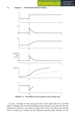
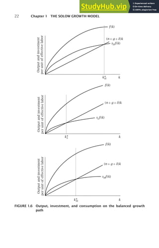
f ′
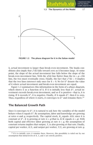
(k∗) can be either smaller or larger than n + g + δ. This is shown in
Figure 1.6. The figure shows not only (n + g+ δ)k and sf (k), but also f (k).
Since consumption on the balanced growth path equals output less break-
even investment (see [1.19]), c∗ is the distance between f (k) and (n + g+ δ)k
at k = k∗. The figure shows the determinants of c∗ for three different values](https://image.slidesharecdn.com/advanced-macroeconomics-230806183016-1212def2/85/Advanced-Macroeconomics-43-320.jpg)
![24 Chapter 1 THE SOLOW GROWTH MODEL
Equation (1.22) holds for all values of s (and of n, g, and δ). Thus the deriva-
tives of the two sides with respect to s are equal:14
sf ′
(k∗)
∂k∗
∂s
+ f (k∗) = (n + g +δ)
∂k∗
∂s
, (1.23)
where the arguments of k∗ are omitted for simplicity. This can be rearranged
to obtain15
∂k∗
∂s
=
f (k∗)
(n + g +δ) − sf ′
(k∗)
. (1.24)
Substituting (1.24) into (1.21) yields
∂y∗
∂s
=
f ′
(k∗)f (k∗)
(n + g +δ) − sf ′
(k∗)
. (1.25)
Two changes help in interpreting this expression. The first is to convert it
to an elasticity by multiplying both sides by s/y∗. The second is to use the
fact that sf (k∗) = (n + g + δ)k∗ to substitute for s. Making these changes
gives us
s
y∗
∂y∗
∂s
=
s
f (k∗)
f ′
(k∗)f (k∗)
(n + g +δ) − sf ′
(k∗)
=
(n + g +δ)k∗f ′
(k∗)
f (k∗)[(n + g +δ) − (n + g +δ)k∗f ′
(k∗)/f (k∗)]
=
k∗f ′
(k∗)/f (k∗)
1 − [k∗f ′
(k∗)/f (k∗)]
.
(1.26)
k∗f ′
(k∗)/f (k∗) is the elasticity of output with respect to capital at k = k∗.
Denoting this by αK (k∗), we have
s
y∗
∂y∗
∂s
=
αK (k∗)
1 − αK (k∗)
. (1.27)
Thus we have found a relatively simple expression for the elasticity of the
balanced-growth-path level of output with respect to the saving rate.
To think about the quantitative implications of (1.27), note that if mar-
kets are competitive and there are no externalities, capital earns its marginal
14
This technique is known as implicit differentiation. Even though (1.22) does not ex-
plicitly give k∗ as a function of s, n, g, and δ, it still determines how k∗ depends on those
variables. We can therefore differentiate the equation with respect to s and solve for ∂k∗/∂s.
15
We saw in the previous section that an increase in s raises k∗. To check that this is
also implied by equation (1.24), note that n + g+ δ is the slope of the break-even investment
line and that sf ′
(k∗) is the slope of the actual investment line at k∗. Since the break-even
investment line is steeper than the actual investment line at k∗ (see Figure 1.2), it follows
that the denominator of (1.24) is positive, and thus that ∂k∗/∂s 0.](https://image.slidesharecdn.com/advanced-macroeconomics-230806183016-1212def2/85/Advanced-Macroeconomics-46-320.jpg)
![1.5 Quantitative Implications 25
product. Since output equals ALf (k) and k equals K/AL, the marginal prod-
uct of capital, ∂Y/∂K, is ALf ′
(k)[1/(AL)], or just f ′
(k). Thus if capital earns its
marginal product, the total amount earned by capital (per unit of effective
labor) on the balanced growth path is k∗f ′
(k∗). The share of total income that
goes to capital on the balanced growth path is then k∗f ′
(k∗)/f (k∗), or αK (k∗).
In other words, if the assumption that capital earns its marginal product is
a good approximation, we can use data on the share of income going to
capital to estimate the elasticity of output with respect to capital, αK (k∗).
In most countries, the share of income paid to capital is about one-third.
If we use this as an estimate of αK (k∗), it follows that the elasticity of output
with respect to the saving rate in the long run is about one-half. Thus, for
example, a 10 percent increase in the saving rate (from 20 percent of output
to 22 percent, for instance) raises output per worker in the long run by about
5 percent relative to the path it would have followed. Even a 50 percent
increase in s raises y∗ only by about 22 percent. Thus significant changes
in saving have only moderate effects on the level of output on the balanced
growth path.
Intuitively, a small value of αK (k∗) makes the impact of saving on output
low for two reasons. First, it implies that the actual investment curve, sf (k),
bends fairly sharply. As a result, an upward shift of the curve moves its
intersection with the break-even investment line relatively little. Thus the
impact of a change in s on k∗ is small. Second, a low value of αK (k∗) means
that the impact of a change in k∗ on y∗ is small.
The Speed of Convergence
In practice, we are interested not only in the eventual effects of some change
(such as a change in the saving rate), but also in how rapidly those effects
occur. Again, we can use approximations around the long-run equilibrium
to address this issue.
For simplicity, we focus on the behavior of k rather than y. Our goal is thus
to determine how rapidly k approaches k∗. We know that ˙
k is determined
by k: recall that the key equation of the model is ˙
k = sf (k) − (n + g + δ)k
(see [1.18]). Thus we can write ˙
k = ˙
k(k). When k equals k∗, ˙
k is zero. A first-
order Taylor-series approximation of ˙
k(k) around k = k∗ therefore yields
˙
k ≃
∂˙
k(k)
∂k
k=k∗
(k − k∗). (1.28)
That is, ˙
k is approximately equal to the product of the difference between
k and k∗ and the derivative of ˙
k with respect to k at k = k∗.
Let λ denote −∂˙
k(k)/∂k|k=k∗ . With this definition, (1.28) becomes
˙
k(t) ≃ −λ[k(t) − k∗]. (1.29)](https://image.slidesharecdn.com/advanced-macroeconomics-230806183016-1212def2/85/Advanced-Macroeconomics-47-320.jpg)
![26 Chapter 1 THE SOLOW GROWTH MODEL
Since ˙
k is positive when k is slightly below k∗ and negative when it is slightly
above, ∂˙
k(k)/∂k|k=k∗ is negative. Equivalently, λ is positive.
Equation (1.29) implies that in the vicinity of the balanced growth path,
k moves toward k∗ at a speed approximately proportional to its distance
from k∗. That is, the growth rate of k(t) − k∗ is approximately constant and
equal to −λ. This implies
k(t) ≃ k∗ + e−λt
[k(0) − k∗], (1.30)
where k(0) is the initial value of k. Note that (1.30) follows just from the
facts that the system is stable (that is, that k converges to k∗) and that we
are linearizing the equation for ˙
k around k = k∗.
It remains to find λ; this is where the specifics of the model enter the anal-
ysis. Differentiating expression (1.18) for ˙
k with respect to k and evaluating
the resulting expression at k = k∗ yields
λ ≡ −
∂˙
k(k)
∂k
k=k∗
= −[sf ′
(k∗) − (n + g +δ)]
= (n + g +δ) − sf ′
(k∗)
= (n + g +δ) −
(n + g + δ)k∗f ′
(k∗)
f (k∗)
= [1 − αK (k∗)](n + g + δ).
(1.31)
Here the third line again uses the fact that sf (k∗) = (n + g + δ)k∗ to sub-
stitute for s, and the last line uses the definition of αK . Thus, k converges
to its balanced-growth-path value at rate [1 − αK (k∗)](n + g+δ). In addition,
one can show that y approaches y∗ at the same rate that k approaches k∗.
That is, y(t) − y∗ ≃ e−λt
[y(0) − y∗].16
We can calibrate (1.31) to see how quickly actual economies are likely to
approach their balanced growth paths. Typically, n+g+δis about 6 percent
per year. This arises, for example, with 1 to 2 percent population growth, 1
to 2 percent growth in output per worker, and 3 to 4 percent depreciation.
If capital’s share is roughly one-third, (1 − αK )(n + g + δ) is thus roughly
4 percent. Therefore k and y move 4 percent of the remaining distance
toward k∗ and y∗ each year, and take approximately 17 years to get halfway
to their balanced-growth-path values.17
Thus in our example of a 10 percent
16
See Problem 1.11.
17
The time it takes for a variable (in this case, y − y∗) with a constant negative growth rate
to fall in half is approximately equal to 70 divided by its growth rate in percent. (Similarly,
the doubling time of a variable with positive growth is 70 divided by the growth rate.) Thus
in this case the half-life is roughly 70/(4%/year), or about 17 years. More exactly, the half-life,
t∗, is the solution to e−λt ∗
= 0.5, where λ is the rate of decrease. Taking logs of both sides,
t∗ = − ln(0.5)/λ ≃ 0.69/λ.](https://image.slidesharecdn.com/advanced-macroeconomics-230806183016-1212def2/85/Advanced-Macroeconomics-48-320.jpg)

![28 Chapter 1 THE SOLOW GROWTH MODEL
X in the vicinity of 10. Our analysis implies that doing this on the basis of
differences in capital requires a difference of a factor of 101/αK
in capital
per worker. For αK = 1
3
, this is a factor of 1000. Even if capital’s share is
one-half, which is well above what data on capital income suggest, one still
needs a difference of a factor of 100.
There is no evidence of such differences in capital stocks. Capital-output
ratios are roughly constant over time. Thus the capital stock per worker in
industrialized countries is roughly 10 times larger than it was 100 years
ago, not 100 or 1000 times larger. Similarly, although capital-output ratios
vary somewhat across countries, the variation is not great. For example,
the capital-output ratio appears to be 2 to 3 times larger in industrialized
countries than in poor countries; thus capital per worker is “only” about 20
to 30 times larger. In sum, differences in capital per worker are far smaller
than those needed to account for the differences in output per worker that
we are trying to understand.
The indirect way of seeing that the model cannot account for large varia-
tions in output per worker on the basis of differences in capital per worker is
to notice that the required differences in capital imply enormous differences
in the rate of return on capital (Lucas, 1990). If markets are competitive, the
rate of return on capital equals its marginal product, f ′
(k), minus depreci-
ation, δ. Suppose that the production function is Cobb–Douglas, which in
intensive form is f (k) = kα
(see equation [1.7]). With this production func-
tion, the elasticity of output with respect to capital is simply α. The marginal
product of capital is
f ′
(k) = αkα−1
= αy (α−1)/α
.
(1.32)
Equation (1.32) implies that the elasticity of the marginal product of cap-
ital with respect to output is −(1 − α)/α. If α= 1
3
, a tenfold difference in
output per worker arising from differences in capital per worker thus im-
plies a hundredfold difference in the marginal product of capital. And since
the return to capital is f ′
(k) − δ, the difference in rates of return is even
larger.
Again, there is no evidence of such differences in rates of return. Direct
measurement of returns on financial assets, for example, suggests only
moderate variation over time and across countries. More tellingly, we can
learn much about cross-country differences simply by examining where the
holders of capital want to invest. If rates of return were larger by a factor of
10 or 100 in poor countries than in rich countries, there would be immense
incentives to invest in poor countries. Such differences in rates of return
would swamp such considerations as capital-market imperfections, govern-
ment tax policies, fear of expropriation, and so on, and we would observe](https://image.slidesharecdn.com/advanced-macroeconomics-230806183016-1212def2/85/Advanced-Macroeconomics-50-320.jpg)

![30 Chapter 1 THE SOLOW GROWTH MODEL
more than just physical capital, or if physical capital has positive external-
ities, then the private return on physical capital is not an accurate guide to
capital’s importance in production. In this case, the calculations we have
done may be misleading, and it may be possible to resuscitate the view that
differences in capital are central to differences in incomes.
These possibilities for addressing the fundamental questions of growth
theory are the subject of Chapters 3 and 4.
1.7 Empirical Applications
Growth Accounting
In many situations, we are interested in the proximate determinants of
growth. That is, we often want to know how much of growth over some
period is due to increases in various factors of production, and how much
stems from other forces. Growth accounting, which was pioneered by
Abramovitz (1956) and Solow (1957), provides a way of tackling this subject.
To see how growth accounting works, consider again the production func-
tion Y(t) = F (K(t),A(t)L(t)). This implies
Ẏ (t) =
∂Y(t)
∂K(t)
K̇(t) +
∂Y(t)
∂L(t)
L̇(t) +
∂Y(t)
∂A(t)
Ȧ(t), (1.33)
where ∂Y/∂L and ∂Y/∂A denote [∂Y/∂(AL)]A and [∂Y/∂(AL)]L, respectively.
Dividing both sides by Y(t) and rewriting the terms on the right-hand side
yields
Ẏ (t)
Y(t)
=
K(t)
Y(t)
∂Y(t)
∂K(t)
K̇(t)
K(t)
+
L(t)
Y(t)
∂Y(t)
∂L(t)
L̇(t)
L(t)
+
A(t)
Y(t)
∂Y(t)
∂A(t)
Ȧ(t)
A(t)
≡ αK (t)
K̇(t)
K(t)
+ αL(t)
L̇(t)
L(t)
+ R(t).
(1.34)
Here αL(t) is the elasticity of output with respect to labor at time t,
αK (t) is again the elasticity of output with respect to capital, and R(t) ≡
[A(t)/Y(t)][∂Y(t)/∂A(t)][Ȧ(t)/A(t)]. Subtracting L̇(t)/L(t) from both sides and
using the fact that αL(t) + αK (t) = 1 (see Problem 1.9) gives an expression
for the growth rate of output per worker:
Ẏ (t)
Y(t)
−
L̇(t)
L(t)
= αK (t)
K̇(t)
K(t)
−
L̇(t)
L(t)
+ R(t). (1.35)
The growth rates of Y, K, and L are straightforward to measure. And we
know that if capital earns its marginal product, αK can be measured using
data on the share of income that goes to capital. R(t) can then be mea-
sured as the residual in (1.35). Thus (1.35) provides a way of decomposing
the growth of output per worker into the contribution of growth of capital
per worker and a remaining term, the Solow residual. The Solow residual](https://image.slidesharecdn.com/advanced-macroeconomics-230806183016-1212def2/85/Advanced-Macroeconomics-52-320.jpg)


![1.7 Empirical Applications 35
regression now produces an estimate of b of −0.566, with a standard error
of 0.144. Thus accounting for the selection bias in Baumol’s procedure elim-
inates about half of the convergence that he finds.
The second problem that DeLong identifies is measurement error. Esti-
mates of real income per capita in 1870 are imprecise. Measurement er-
ror again creates bias toward finding convergence. When 1870 income is
overstated, growth over the period 1870–1979 is understated by an equal
amount; when 1870 income is understated, the reverse occurs. Thus mea-
sured growth tends to be lower in countries with higher measured initial
income even if there is no relation between actual growth and actual initial
income.
DeLong therefore considers the following model:
ln
Y
N
i,1979
− ln
Y
N
i,1870
∗
= a + b ln
Y
N
i,1870
∗
+ εi , (1.38)
ln
Y
N
i,1870
= ln
Y
N
i,1870
∗
+ ui . (1.39)
Here ln[(Y/N)1870]∗ is the true value of log income per capita in 1870 and
ln[(Y/N)1870] is the measured value. ε and u are assumed to be uncorrelated
with each other and with ln[(Y/N)1870]∗.
Unfortunately, it is not possible to estimate this model using only data
on ln[(Y/N)1870] and ln[(Y/N)1979]. The problem is that there are different
hypotheses that make identical predictions about the data. For example,
suppose we find that measured growth is negatively related to measured
initial income. This is exactly what one would expect either if measurement
error is unimportant and there is true convergence or if measurement error
is important and there is no true convergence. Technically, the model is not
identified.
DeLong argues, however, that we have at least a rough idea of how good
the 1870 data are, and thus have a sense of what is a reasonable value
for the standard deviation of the measurement error. For example, σu =
0.01 implies that we have measured initial income to within an average of
1 percent; this is implausibly low. Similarly, σu = 0.50—an average error
of 50 percent—seems implausibly high. DeLong shows that if we fix a value
of σu , we can estimate the remaining parameters.
Even moderate measurement error has a substantial impact on the re-
sults. For the unbiased sample, the estimate of b reaches 0 (no tendency
toward convergence) for σu ≃ 0.15, and is 1 (tremendous divergence) for
σu ≃ 0.20. Thus plausible amounts of measurement error eliminate most or
all of the remainder of Baumol’s estimate of convergence.
It is also possible to investigate convergence for different samples of
countries and different time periods. Figure 1.9 is a convergence scatterplot
analogous to Figures 1.7 and 1.8 for virtually the entire non-Communist](https://image.slidesharecdn.com/advanced-macroeconomics-230806183016-1212def2/85/Advanced-Macroeconomics-57-320.jpg)


![1.8 The Environment and Economic Growth 39
production. Thus the production function, (1.1), becomes
Y(t) = K(t)α
R(t)β
T(t)γ
[A(t)L(t)]1−α−β−γ
,
α 0, β 0, γ 0, α + β + γ 1.
(1.41)
Here R denotes resources used in production, and T denotes the amount of
land.
The dynamics of capital, labor, and the effectiveness of labor are the
same as before: K̇(t) = sY(t) − δK(t), L̇(t) = nL(t), and Ȧ(t) = gA(t). The new
assumptions concern resources and land. Since the amount of land on earth
is fixed, in the long run the quantity used in production cannot be growing.
Thus we assume
Ṫ (t) = 0. (1.42)
Similarly, the facts that resource endowments are fixed and that resources
are used in production imply that resource use must eventually decline.
Thus, even though resource use has been rising historically, we assume
Ṙ(t) = −bR(t), b 0. (1.43)
The presence of resources and land in the production function means
that K/AL no longer converges to some value. As a result, we cannot use
our previous approach of focusing on K/AL to analyze the behavior of this
economy. A useful strategy in such situations is to ask whether there can be
a balanced growth path and, if so, what the growth rates of the economy’s
variables are on that path.
By assumption, A, L, R, and T are each growing at a constant rate. Thus
what is needed for a balanced growth path is that K and Y each grow at
a constant rate. The equation of motion for capital, K̇(t) = sY(t) − δK(t),
implies that the growth rate of K is
K̇(t)
K(t)
= s
Y(t)
K(t)
− δ. (1.44)
Thus for the growth rate of K to be constant, Y/K must be constant. That
is, the growth rates of Y and K must be equal.
We can use the production function, (1.41), to find when this can occur.
Taking logs of both sides of (1.41) gives us
ln Y(t) = αln K(t) + βln R(t) + γ ln T(t)
+ (1 − α − β − γ )[ln A(t) + ln L(t)].
(1.45)
We can now differentiate both sides of this expression with respect to time.
Using the fact that the time derivative of the log of a variable equals the
variable’s growth rate, we obtain
gY (t) = αgK (t) + βgR(t) + γgT (t) + (1 − α − β − γ )[gA (t) + gL(t)], (1.46)](https://image.slidesharecdn.com/advanced-macroeconomics-230806183016-1212def2/85/Advanced-Macroeconomics-61-320.jpg)
![1.8 The Environment and Economic Growth 41
An Illustrative Calculation
In recent history, the advantages of technological progress have outweighed
the disadvantages of resource and land limitations. But this does not tell us
how large those disadvantages are. For example, they might be large enough
that only a moderate slowing of technological progress would make overall
growth in income per worker negative.
Resource and land limitations reduce growth by causing resource use per
worker and land per worker to be falling. Thus, as Nordhaus (1992) observes,
to gauge how much these limitations are reducing growth, we need to ask
how much greater growth would be if resources and land per worker were
constant. Concretely, consider an economy identical to the one we have
just considered except that the assumptions Ṫ (t) = 0 and Ṙ(t) = −bR(t)
are replaced with the assumptions Ṫ (t) = nT (t) and Ṙ(t) = nR(t). In this
hypothetical economy, there are no resource and land limitations; both grow
as population grows. Analysis parallel to that used to derive equation (1.49)
shows that growth of output per worker on the balanced growth path of
this economy is24
g̃
bgp
Y/L =
1
1 − α
(1 − α − β − γ )g. (1.50)
The “growth drag” from resource and land limitations is the difference
between growth in this hypothetical case and growth in the case of resource
and land limitations:
Drag = g̃
bgp
Y/L − g
bgp
Y/L
=
(1 − α − β − γ )g − [(1 − α − β − γ )g − βb− (β + γ )n]
1 − α
=
βb+ (β + γ )n
1 − α
.
(1.51)
Thus, the growth drag is increasing in resources’ share (β), land’s share (γ ),
the rate that resource use is falling (b), the rate of population growth (n),
and capital’s share (α).
It is possible to quantify the size of the drag. Because resources and land
are traded in markets, we can use income data to estimate their importance
in production—that is, to estimate β and γ . As Nordhaus (1992) describes,
these data suggest a combined value of β + γ of about 0.2. Nordhaus goes
on to use a somewhat more complicated version of the framework pre-
sented here to estimate the growth drag. His point estimate is a drag of
0.0024—that is, about a quarter of a percentage point per year. He finds
that only about a quarter of the drag is due to the limited supply of land. Of
24
See Problem 1.15.](https://image.slidesharecdn.com/advanced-macroeconomics-230806183016-1212def2/85/Advanced-Macroeconomics-63-320.jpg)


![Problems 45
Of course, it is possible that this reading of the scientific evidence or this
effort to estimate welfare effects is far from the mark. It is also possible
that considering horizons longer than the 50 to 100 years usually examined
in such studies would change the conclusions substantially. But the fact
remains that most economists who have studied environmental issues seri-
ously, even ones whose initial positions were sympathetic to environmental
concerns, have concluded that the likely impact of environmental problems
on growth is at most moderate.26
Problems
1.1. Basic properties of growth rates. Use the fact that the growth rate of a variable
equals the time derivative of its log to show:
(a) The growth rate of the product of two variables equals the sum of
their growth rates. That is, if Z(t) = X(t)Y (t), then Ż(t)/Z(t) = [Ẋ (t)/X(t)] +
[Ẏ (t)/Y (t)].
(b) The growth rate of the ratio of two variables equals the difference of their
growth rates. That is, if Z(t) = X(t)/Y (t), then Ż(t)/Z(t) = [Ẋ (t)/X(t)] −
[Ẏ (t)/Y (t)].
(c) If Z(t) = X(t)α
, then Ż(t)/Z(t) = αẊ (t)/X(t).
1.2. Suppose that the growth rate of some variable, X, is constant and equal to
a 0 from time 0 to time t1; drops to 0 at time t1; rises gradually from 0 to a
from time t1 to time t2; and is constant and equal to a after time t2.
(a) Sketch a graph of the growth rate of X as a function of time.
(b) Sketch a graph of ln X as a function of time.
1.3. Describe how, if at all, each of the following developments affects the break-
even and actual investment lines in our basic diagram for the Solow model:
(a) The rate of depreciation falls.
(b) The rate of technological progress rises.
(c) The production function is Cobb–Douglas, f (k) = kα
, and capital’s share,
α, rises.
(d) Workers exert more effort, so that output per unit of effective labor for a
given value of capital per unit of effective labor is higher than before.
26
This does not imply that environmental factors are always unimportant to long-run
growth. Brander and Taylor (1998) make a strong case that Easter Island suffered an envi-
ronmental disaster of the type envisioned by Malthusians sometime between its settlement
around 400 and the arrival of Europeans in the 1700s. And they argue that other primitive
societies may have also suffered such disasters.](https://image.slidesharecdn.com/advanced-macroeconomics-230806183016-1212def2/85/Advanced-Macroeconomics-67-320.jpg)
![46 Chapter 1 THE SOLOW GROWTH MODEL
1.4. Consider an economy with technological progress but without population
growth that is on its balanced growth path. Now suppose there is a one-time
jump in the number of workers.
(a) At the time of the jump, does output per unit of effective labor rise, fall,
or stay the same? Why?
(b) After the initial change (if any) in output per unit of effective labor when
the new workers appear, is there any further change in output per unit of
effective labor? If so, does it rise or fall? Why?
(c) Once the economy has again reached a balanced growth path, is output
per unit of effective labor higher, lower, or the same as it was before the
new workers appeared? Why?
1.5. Suppose that the production function is Cobb–Douglas.
(a) Find expressions for k∗, y∗, and c ∗ as functions of the parameters of the
model, s, n, δ, g, and α.
(b) What is the golden-rule value of k?
(c) What saving rate is needed to yield the golden-rule capital stock?
1.6. Consider a Solow economy that is on its balanced growth path. Assume for
simplicity that there is no technological progress. Now suppose that the rate
of population growth falls.
(a) What happens to the balanced-growth-path values of capital per worker,
output per worker, and consumption per worker? Sketch the paths of these
variables as the economy moves to its new balanced growth path.
(b) Describe the effect of the fall in population growth on the path of output
(that is, total output, not output per worker).
1.7. Find the elasticity of output per unit of effective labor on the balanced growth
path, y∗, with respect to the rate of population growth, n. If αK (k∗) = 1
3
,
g = 2%, and δ = 3%, by about how much does a fall in n from 2 percent to
1 percent raise y∗?
1.8. Suppose that investment as a fraction of output in the United States rises
permanently from 0.15 to 0.18. Assume that capital’s share is 1
3
.
(a) By about how much does output eventually rise relative to what it would
have been without the rise in investment?
(b) By about how much does consumption rise relative to what it would have
been without the rise in investment?
(c) What is the immediate effect of the rise in investment on consumption?
About how long does it take for consumption to return to what it would
have been without the rise in investment?
1.9. Factor payments in the Solow model. Assume that both labor and capital
are paid their marginal products. Let w denote ∂F (K, AL)/∂L and r denote
[∂F (K,AL)/∂K] − δ.
(a) Show that the marginal product of labor, w, is A[f (k) − kf ′
(k)].](https://image.slidesharecdn.com/advanced-macroeconomics-230806183016-1212def2/85/Advanced-Macroeconomics-68-320.jpg)
![Problems 47
(b) Show that if both capital and labor are paid their marginal products, con-
stant returns to scale imply that the total amount paid to the factors of
production equals total net output. That is, show that under constant
returns, wL + rK = F (K,AL) − δK.
(c) The return to capital (r) is roughly constant over time, as are the shares of
output going to capital and to labor. Does a Solow economy on a balanced
growth path exhibit these properties? What are the growth rates of w and
r on a balanced growth path?
(d) Suppose the economy begins with a level of k less than k∗. As k moves
toward k∗, is w growing at a rate greater than, less than, or equal to its
growth rate on the balanced growth path? What about r ?
1.10. Suppose that, as in Problem 1.9, capital and labor are paid their marginal
products. In addition, suppose that all capital income is saved and all labor
income is consumed. Thus K̇ = [∂F (K,AL)/∂K]K − δK.
(a) Show that this economy converges to a balanced growth path.
(b) Is k on the balanced growth path greater than, less than, or equal to the
golden-rule level of k? What is the intuition for this result?
1.11. Go through steps analogous to those in equations (1.28)–(1.31) to find how
quickly y converges to y∗ in the vicinity of the balanced growth path. (Hint:
Since y = f (k), we can write k = g(y), where g(•) = f −1
(•).)
1.12. Embodied technological progress. (This follows Solow, 1960, and Sato, 1966.)
One view of technological progress is that the productivity of capital goods
built at t depends on the state of technology at t and is unaffected by subse-
quent technological progress. This is known as embodied technological pro-
gress (technological progress must be “embodied” in new capital before it can
raise output). This problem asks you to investigate its effects.
(a) As a preliminary, let us modify the basic Solow model to make technolog-
ical progress capital-augmenting rather than labor-augmenting. So that
a balanced growth path exists, assume that the production function is
Cobb–Douglas: Y (t) = [A(t)K(t)]α
L(t)1−α
. Assume that A grows at rate
μ: Ȧ(t) = μA(t).
Show that the economy converges to a balanced growth path, and find
the growth rates of Y and K on the balanced growth path. (Hint: Show that
we can write Y/(Aφ
L) as a function of K/(Aφ
L), where φ = α/(1−α). Then
analyze the dynamics of K/(Aφ
L).)
(b) Now consider embodied technological progress. Specifically, let the pro-
duction function be Y (t) = J(t)α
L(t)1−α
, where J(t) is the effective capital
stock. The dynamics of J(t) are given by ˙
J (t) = sA(t)Y (t)− δJ(t). The pres-
ence of the A(t) term in this expression means that the productivity of
investment at t depends on the technology at t.
Show that the economy converges to a balanced growth path. What
are the growth rates of Y and J on the balanced growth path? (Hint: Let
J(t) = J(t)/A(t). Then use the same approach as in (a), focusing on J/(Aφ
L)
instead of K/(Aφ
L).)](https://image.slidesharecdn.com/advanced-macroeconomics-230806183016-1212def2/85/Advanced-Macroeconomics-69-320.jpg)
![48 Chapter 1 THE SOLOW GROWTH MODEL
(c) What is the elasticity of output on the balanced growth path with respect
to s?
(d) In the vicinity of the balanced growth path, how rapidly does the economy
converge to the balanced growth path?
(e) Compare your results for (c) and (d ) with the corresponding results in the
text for the basic Solow model.
1.13. Consider a Solow economy on its balanced growth path. Suppose the growth-
accounting techniques described in Section 1.7 are applied to this economy.
(a) What fraction of growth in output per worker does growth accounting
attribute to growth in capital per worker? What fraction does it attribute
to technological progress?
(b) How can you reconcile your results in (a) with the fact that the Solow
model implies that the growth rate of output per worker on the balanced
growth path is determined solely by the rate of technological progress?
1.14. (a) In the model of convergence and measurement error in equations (1.38)
and (1.39), suppose the true value of b is −1. Does a regression of
ln(Y/N )1979 − ln(Y/N )1870 on a constant and ln(Y/N )1870 yield a biased
estimate of b? Explain.
(b) Suppose there is measurement error in measured 1979 income per capita
but not in 1870 income per capita. Does a regression of ln(Y/N )1979 −
ln(Y/N )1870 on a constant and ln(Y/N )1870 yield a biased estimate of b?
Explain.
1.15. Derive equation (1.50). (Hint: Follow steps analogous to those in equations
[1.47] and [1.48].)](https://image.slidesharecdn.com/advanced-macroeconomics-230806183016-1212def2/85/Advanced-Macroeconomics-70-320.jpg)
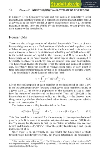
![2.2 The Behavior of Households and Firms 51
willingness to shift consumption between different periods. When θ is
smaller, marginal utility falls more slowly as consumption rises, and so the
household is more willing to allow its consumption to vary over time. If θ
is close to zero, for example, utility is almost linear in C, and so the house-
hold is willing to accept large swings in consumption to take advantage of
small differences between the discount rate and the rate of return on sav-
ing. Specifically, one can show that the elasticity of substitution between
consumption at any two points in time is 1/θ.2
Three additional features of the instantaneous utility function are worth
mentioning. First, C1−θ
is increasing in C if θ 1 but decreasing if θ 1;
dividing C1−θ
by 1 − θ thus ensures that the marginal utility of consump-
tion is positive regardless of the value of θ. Second, in the special case
of θ → 1, the instantaneous utility function simplifies to ln C; this is of-
ten a useful case to consider.3
And third, the assumption that ρ − n −
(1 − θ)g 0 ensures that lifetime utility does not diverge: if this condi-
tion does not hold, the household can attain infinite lifetime utility, and its
maximization problem does not have a well-defined solution.4
2.2 The Behavior of Households and
Firms
Firms
Firms’ behavior is relatively simple. At each point in time they employ the
stocks of labor and capital, pay them their marginal products, and sell the
resulting output. Because the production function has constant returns and
the economy is competitive, firms earn zero profits.
As described in Chapter 1, the marginal product of capital, ∂F (K,AL)/∂K,
is f ′
(k), where f (•) is the intensive form of the production function. Because
markets are competitive, capital earns its marginal product. And because
there is no depreciation, the real rate of return on capital equals its earnings
per unit time. Thus the real interest rate at time t is
r(t) = f ′
(k (t)). (2.3)
Labor’s marginal product is ∂F (K,AL)/∂L, which equals A∂F (K,AL)/
∂AL. In terms of f (•), this is A[f (k) − kf ′
(k)].5
Thus the real wage
2
See Problem 2.2.
3
To see this, first subtract 1/(1−θ) from the utility function; since this changes utility by
a constant, it does not affect behavior. Then take the limit as θ approaches 1; this requires
using l’Hôpital’s rule. The result is ln C.
4
Phelps (1966a) discusses how growth models can be analyzed when households can
obtain infinite utility.
5
See Problem 1.9.](https://image.slidesharecdn.com/advanced-macroeconomics-230806183016-1212def2/85/Advanced-Macroeconomics-73-320.jpg)
![52 Chapter 2 INFINITE HORIZONS AND OVERLAPPING GENERATIONS
at t is
W(t) = A(t)[f (k (t)) − k (t)f ′
(k (t))]. (2.4)
The wage per unit of effective labor is therefore
w(t) = f (k (t)) − k (t)f ′
(k (t)). (2.5)
Households’ Budget Constraint
The representative household takes the paths of r and w as given. Its bud-
get constraint is that the present value of its lifetime consumption cannot
exceed its initial wealth plus the present value of its lifetime labor income.
To write the budget constraint formally, we need to account for the fact that
r may vary over time. To do this, define R(t) as
t
τ= 0
r(τ) dτ. One unit of the
output good invested at time 0 yields eR(t )
units of the good at t; equiva-
lently, the value of 1 unit of output at time t in terms of output at time 0 is
e−R(t )
. For example, if r is constant at some level r, R(t) is simply rt and the
present value of 1 unit of output at t is e−rt
. More generally, eR(t )
shows the
effects of continuously compounding interest over the period [0,t].
Since the household has L(t)/H members, its labor income at t is
W(t)L(t)/H, and its consumption expenditures are C(t)L(t)/H. Its initial
wealth is 1/H of total wealth at time 0, or K(0)/H. The household’s bud-
get constraint is therefore
∞
t =0
e−R(t )
C(t)
L(t)
H
dt ≤
K(0)
H
+
∞
t =0
e−R(t )
W(t)
L(t)
H
dt. (2.6)
In general, it is not possible to find the integrals in this expression. Fortu-
nately, we can express the budget constraint in terms of the limiting behav-
ior of the household’s capital holdings; and it is usually possible to describe
the limiting behavior of the economy. To see how the budget constraint can
be rewritten in this way, first bring all the terms of (2.6) over to the same
side and combine the two integrals; this gives us
K(0)
H
+
∞
t =0
e−R(t )
[W(t) − C(t)]
L(t)
H
dt ≥ 0. (2.7)
We can write the integral from t = 0 to t = ∞ as a limit. Thus (2.7) is
equivalent to
lim
s→∞
K(0)
H
+
s
t =0
e−R(t )
[W(t) − C(t)]
L(t)
H
dt
≥ 0. (2.8)](https://image.slidesharecdn.com/advanced-macroeconomics-230806183016-1212def2/85/Advanced-Macroeconomics-74-320.jpg)
![2.2 The Behavior of Households and Firms 53
Now note that the household’s capital holdings at time s are
K(s)
H
= eR(s) K(0)
H
+
s
t =0
eR(s)−R(t )
[W(t) − C(t)]
L(t)
H
dt. (2.9)
To understand (2.9), observe that eR(s)
K(0)/H is the contribution of the
household’s initial wealth to its wealth at s. The household’s saving at t is
[W(t) − C(t)]L(t)/H (which may be negative); eR(s)−R(t )
shows how the value
of that saving changes from t to s.
The expression in (2.9) is eR(s)
times the expression in brackets in (2.8).
Thus we can write the budget constraint as simply
lim
s→∞
e−R(s) K(s)
H
≥ 0. (2.10)
Expressed in this form, the budget constraint states that the present value
of the household’s asset holdings cannot be negative in the limit.
Equation (2.10) is known as the no-Ponzi-game condition. A Ponzi game
is a scheme in which someone issues debt and rolls it over forever. That is,
the issuer always obtains the funds to pay off debt when it comes due by
issuing new debt. Such a scheme allows the issuer to have a present value of
lifetime consumption that exceeds the present value of his or her lifetime
resources. By imposing the budget constraint (2.6) or (2.10), we are ruling
out such schemes.6
Households’ Maximization Problem
The representative household wants to maximize its lifetime utility subject
to its budget constraint. As in the Solow model, it is easier to work with
variables normalized by the quantity of effective labor. To do this, we need
to express both the objective function and the budget constraint in terms
of consumption and labor income per unit of effective labor.
6
This analysis sweeps a subtlety under the rug: we have assumed rather than shown that
households must satisfy the no-Ponzi-game condition. Because there are a finite number
of households in the model, the assumption that Ponzi games are not feasible is correct. A
household can run a Ponzi game only if at least one other household has a present value of
lifetime consumption that is strictly less than the present value of its lifetime wealth. Since
the marginal utility of consumption is always positive, no household will accept this. But
in models with infinitely many households, such as the overlapping-generations model of
Part B of this chapter, Ponzi games are possible in some situations. We return to this point
in Section 12.1.](https://image.slidesharecdn.com/advanced-macroeconomics-230806183016-1212def2/85/Advanced-Macroeconomics-75-320.jpg)
![54 Chapter 2 INFINITE HORIZONS AND OVERLAPPING GENERATIONS
We start with the objective function. Define c (t) to be consumption per
unit of effective labor. Thus C(t), consumption per worker, equals A(t)c (t).
The household’s instantaneous utility, (2.2), is therefore
C(t)1−θ
1 − θ
=
[A(t)c (t)]1−θ
1 − θ
=
[A(0)egt
]1−θ
c (t)1−θ
1 − θ
= A(0)1−θ
e(1−θ)gt c (t)1−θ
1 − θ
.
(2.11)
Substituting (2.11) and the fact that L(t) = L(0)ent
into the household’s
objective function, (2.1)–(2.2), yields
U =
∞
t =0
e−ρt C(t)1−θ
1 − θ
L(t)
H
dt
=
∞
t =0
e−ρt
A(0)1−θ
e(1−θ)gt c (t)1−θ
1 − θ
L(0)ent
H
dt
= A(0)1−θ L(0)
H
∞
t =0
e−ρt
e(1−θ)gt
en t c (t)1−θ
1 − θ
dt
≡ B
∞
t =0
e−βt c (t)1−θ
1 − θ
dt,
(2.12)
where B ≡ A(0)1−θ
L(0)/H and β ≡ ρ − n − (1 − θ)g. From (2.2), β is assumed
to be positive.
Now consider the budget constraint, (2.6). The household’s total con-
sumption at t, C(t)L(t)/H, equals consumption per unit of effective labor,
c (t), times the household’s quantity of effective labor, A(t)L(t)/H. Similarly,
its total labor income at t equals the wage per unit of effective labor, w(t),
times A(t)L(t)/H. And its initial capital holdings are capital per unit of ef-
fective labor at time 0, k (0), times A(0)L(0)/H. Thus we can rewrite (2.6) as
∞
t =0
e−R(t )
c (t)
A(t)L(t)
H
dt
≤ k (0)
A(0)L(0)
H
+
∞
t =0
e−R(t )
w(t)
A(t)L(t)
H
dt.
(2.13)
A(t)L(t) equals A(0)L(0)e(n +g)t
. Substituting this fact into (2.13) and dividing
both sides by A(0)L(0)/H yields
∞
t =0
e−R(t )
c (t)e(n +g)t
dt ≤ k (0) +
∞
t =0
e−R(t )
w(t)e(n +g)t
dt. (2.14)](https://image.slidesharecdn.com/advanced-macroeconomics-230806183016-1212def2/85/Advanced-Macroeconomics-76-320.jpg)
![2.2 The Behavior of Households and Firms 55
Finally, because K(s) is proportional to k (s)e(n +g)s
, we can rewrite the
no-Ponzi-game version of the budget constraint, (2.10), as
lim
s→∞
e−R(s)
e(n +g)s
k (s) ≥ 0. (2.15)
Household Behavior
The household’s problem is to choose the path of c (t) to maximize life-
time utility, (2.12), subject to the budget constraint, (2.14). Although this
involves choosing c at each instant of time (rather than choosing a finite
set of variables, as in standard maximization problems), conventional max-
imization techniques can be used. Since the marginal utility of consumption
is always positive, the household satisfies its budget constraint with equal-
ity. We can therefore use the objective function, (2.12), and the budget con-
straint, (2.14), to set up the Lagrangian:
L = B
∞
t =0
e−βt c (t)1−θ
1 − θ
dt
(2.16)
+ λ
k (0) +
∞
t =0
e−R(t )
e(n +g)t
w(t) dt −
∞
t =0
e−R(t )
e(n +g)t
c (t) dt
.
The household chooses c at each point in time; that is, it chooses infinitely
many c (t)’s. The first-order condition for an individual c (t) is7
Be−βt
c (t)−θ
= λe−R(t )
e(n +g)t
. (2.17)
The household’s behavior is characterized by (2.17) and the budget con-
straint, (2.14).
7
This step is slightly informal; the difficulty is that the terms in (2.17) are of order dt in
(2.16); that is, they make an infinitesimal contribution to the Lagrangian. There are various
ways of addressing this issue more formally than simply “canceling” the dt’s (which is what
we do in [2.17]). For example, we can model the household as choosing consumption over the
finite intervals [0,t), [t,2t), [2t,3t), . . . , with its consumption required to be constant
within each interval, and then take the limit as t approaches zero. This also yields (2.17).
Another possibility is to use the calculus of variations (see n. 13, at the end of Section 2.4).
In this particular application, however, the calculus-of-variations approach simplifies to the
approach we have used here. That is, here the calculus-of-variations approach is no more
rigorous than the approach we have used. To put it differently, the methods used to derive
the calculus of variations provide a formal justification for canceling the dt’s in (2.17).](https://image.slidesharecdn.com/advanced-macroeconomics-230806183016-1212def2/85/Advanced-Macroeconomics-77-320.jpg)
![2.3 The Dynamics of the Economy 57
infinitesimal) period of time t, and then consuming the proceeds at time
t + t; assume that when it does this, the household leaves consumption
and capital holdings at all times other than t and t + t unchanged. If the
household is optimizing, the marginal impact of this change on lifetime
utility must be zero. If the impact is strictly positive, the household can
marginally raise its lifetime utility by making the change. And if the impact
is strictly negative, the household can raise its lifetime utility by making the
opposite change.
From (2.12), the marginal utility of c (t) is Be−βt
c (t)−θ
. Thus the change has
a utility cost of Be−βt
c (t)−θ
c. Since the instantaneous rate of return is r(t), c
at time t+t can be increased by e[r (t )−n−g]t
c. Similarly, since c is growing
at rate ċ (t)/c (t), we can write c (t + t) as c (t)e[ċ (t )/c(t )]t
. Thus the marginal
utility of c (t + t) is Be−β(t +t )
c (t + t)−θ
, or Be−β(t +t )
[c (t)e[ċ(t )/c(t )]t
]−θ
.
For the path of consumption to be utility-maximizing, it must therefore
satisfy
Be−βt
c (t)−θ
c = Be−β(t +t )
[c (t)e[ċ (t )/c(t )]t
]−θ
e[r (t )−n−g]t
c. (2.22)
Dividing by Be−βt
c (t)−θ
c and taking logs yields
−βt − θ
ċ (t)
c (t)
t + [r(t) − n − g] t = 0. (2.23)
Finally, dividing by t and rearranging yields the Euler equation in (2.20).
Intuitively, the Euler equation describes how c must behave over time
given c (0): if c does not evolve according to (2.20), the household can re-
arrange its consumption in a way that raises its lifetime utility without
changing the present value of its lifetime spending. The choice of c (0) is then
determined by the requirement that the present value of lifetime consump-
tion over the resulting path equals initial wealth plus the present value of
future earnings. When c (0) is chosen too low, consumption spending along
the path satisfying (2.20) does not exhaust lifetime wealth, and so a higher
path is possible; when c (0) is set too high, consumption spending more than
uses up lifetime wealth, and so the path is not feasible.9
2.3 The Dynamics of the Economy
The most convenient way to describe the behavior of the economy is in
terms of the evolution of c and k.
9
Formally, equation (2.20) implies that c (t) = c (0)e[R (t ) − (ρ+ θg)t ]/θ
, which implies
that e−R (t )
e(n +g)t
c (t) = c (0)e[(1−θ)R (t )+(θn−ρ)t ]/θ
. Thus c (0) is determined by the fact that
c (0)
∞
t =0
e[(1−θ)R (t ) + (θn − ρ)t ]/θ
dt must equal the right-hand side of the budget constraint,
(2.14).](https://image.slidesharecdn.com/advanced-macroeconomics-230806183016-1212def2/85/Advanced-Macroeconomics-79-320.jpg)
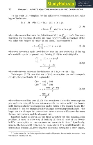
![60 Chapter 2 INFINITE HORIZONS AND OVERLAPPING GENERATIONS
E
c
k∗ k
= 0
k
.
c
.
= 0
FIGURE 2.3 The dynamics of c and k
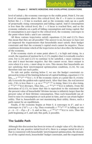
the arrow points to the left. Finally, at Point E both ċ and ˙
k are zero; thus
there is no movement from this point.11
Figure 2.3 is drawn with k∗ (the level of k that implies ċ = 0) less than
the golden-rule level of k (the value of k associated with the peak of the
˙
k = 0 locus). To see that this must be the case, recall that k∗ is defined by
f ′
(k∗) = ρ + θg, and that the golden-rule k is defined by f ′
(kGR) = n + g.
Since f ′′
(k) is negative, k∗ is less than kGR if and only if ρ + θg is greater
than n + g. This is equivalent to ρ−n−(1−θ)g 0, which we have assumed
to hold so that lifetime utility does not diverge (see [2.2]). Thus k∗ is to the
left of the peak of the ˙
k = 0 curve.
The Initial Value of c
Figure 2.3 shows how c and k must evolve over time to satisfy households’
intertemporal optimization condition (equation [2.24]) and the equation
11
Recall from n. 10 that ċ is also zero along the horizontal axis of the phase diagram.
As a result, there are two other points where c and k are constant. The first is the origin: if
the economy has no capital and no consumption, it remains there. The second is the point
where the ˙
k = 0 curve crosses the horizontal axis. Here all of output is being used to hold
k constant, so c = 0 and f (k) = (n + g)k. Since having consumption change from zero to
any positive amount violates households’ intertemporal optimization condition, (2.24), if
the economy is at this point it must remain there to satisfy (2.24) and (2.25). We will see
shortly, however, that the economy is never at either of these points.](https://image.slidesharecdn.com/advanced-macroeconomics-230806183016-1212def2/85/Advanced-Macroeconomics-82-320.jpg)
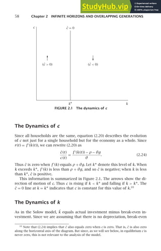
![2.3 The Dynamics of the Economy 61
E
A
B
C
F
D
k(0)
c
k∗ k
c
.
= 0
= 0
k
.
FIGURE 2.4 The behavior of c and k for various initial values of c
relating the change in k to output and consumption (equation [2.25]) given
initial values of c and k. The initial value of k is given; but the initial value
of c must be determined.
This issue is addressed in Figure 2.4. For concreteness, k (0) is assumed
to be less than k∗. The figure shows the trajectory of c and k for various
assumptions concerning the initial level of c. If c (0) is above the ˙
k = 0 curve,
at a point like A, then ċ is positive and ˙
k negative; thus the economy moves
continually up and to the left in the diagram. If c (0) is such that ˙
k is initially
zero (Point B), the economy begins by moving directly up in (k,c) space;
thereafter ċ is positive and ˙
k negative, and so the economy again moves
up and to the left. If the economy begins slightly below the ˙
k = 0 locus
(Point C), ˙
k is initially positive but small (since ˙
k is a continuous function
of c), and ċ is again positive. Thus in this case the economy initially moves
up and slightly to the right; after it crosses the ˙
k = 0 locus, however, ˙
k
becomes negative and once again the economy is on a path of rising c and
falling k.
Point D shows a case of very low initial consumption. Here ċ and ˙
k are
both initially positive. From (2.24), ċ is proportional to c; when c is small,
ċ is therefore small. Thus c remains low, and so the economy eventually
crosses the ċ = 0 line. After this point, ċ becomes negative, and ˙
k remains
positive. Thus the economy moves down and to the right.
ċ and ˙
k are continuous functions of c and k. Thus there is some critical
point between Points C and D—Point F in the diagram—such that at that](https://image.slidesharecdn.com/advanced-macroeconomics-230806183016-1212def2/85/Advanced-Macroeconomics-83-320.jpg)

![2.5 The Balanced Growth Path 65
labor remains the only source of persistent growth in output per worker.
And since the production function is the same as in the Solow model, one
can repeat the calculations of Section 1.6 demonstrating that significant
differences in output per worker can arise from differences in capital per
worker only if the differences in capital per worker, and in rates of return
to capital, are enormous.
The Social Optimum and the Golden-Rule Level of
Capital
The only notable difference between the balanced growth paths of the Solow
and Ramsey–Cass–Koopmans models is that a balanced growth path with a
capital stock above the golden-rule level is not possible in the Ramsey–Cass–
Koopmans model. In the Solow model, a sufficiently high saving rate causes
the economy to reach a balanced growth path with the property that there
are feasible alternatives that involve higher consumption at every moment.
In the Ramsey–Cass–Koopmans model, in contrast, saving is derived from
the behavior of households whose utility depends on their consumption,
and there are no externalities. As a result, it cannot be an equilibrium for
the economy to follow a path where higher consumption can be attained in
every period; if the economy were on such a path, households would reduce
their saving and take advantage of this opportunity.
This can be seen in the phase diagram. Consider again Figure 2.5. If the
initial capital stock exceeds the golden-rule level (that is, if k (0) is greater
than the k associated with the peak of the ˙
k = 0 locus), initial consumption
is above the level needed to keep k constant; thus ˙
k is negative. k gradually
approaches k∗, which is below the golden-rule level.
Finally, the fact that k∗ is less than the golden-rule capital stock implies
that the economy does not converge to the balanced growth path that yields
the maximum sustainable level of c. The intuition for this result is clearest
in the case of g equal to zero, so that there is no long-run growth of con-
sumption and output per worker. In this case, k∗ is defined by f ′
(k∗) = ρ
(see [2.24]) and kGR is defined by f ′
(kGR) = n, and our assumption that
ρ − n − (1 − θ)g 0 simplifies to ρ n. Since k∗ is less than kGR, an in-
crease in saving starting at k = k∗ would cause consumption per worker to
eventually rise above its previous level and remain there (see Section 1.4).
But because households value present consumption more than future con-
sumption, the benefit of the eventual permanent increase in consumption
is bounded. At some point—specifically, when k exceeds k∗—the tradeoff
between the temporary short-term sacrifice and the permanent long-term
gain is sufficiently unfavorable that accepting it reduces rather than raises
lifetime utility. Thus k converges to a value below the golden-rule level. Be-
cause k∗ is the optimal level of k for the economy to converge to, it is known
as the modified golden-rule capital stock.](https://image.slidesharecdn.com/advanced-macroeconomics-230806183016-1212def2/85/Advanced-Macroeconomics-87-320.jpg)
![66 Chapter 2 INFINITE HORIZONS AND OVERLAPPING GENERATIONS
2.6 The Effects of a Fall in the Discount
Rate
Consider a Ramsey–Cass–Koopmans economy that is on its balanced growth
path, and suppose that there is a fall in ρ, the discount rate. Because ρ is the
parameter governing households’ preferences between current and future
consumption, this change is the closest analogue in this model to a rise in
the saving rate in the Solow model.
Since the division of output between consumption and investment is
determined by forward-looking households, we must specify whether the
change is expected or unexpected. If a change is expected, households may
alter their behavior before the change occurs. We therefore focus on the
simple case where the change is unexpected. That is, households are opti-
mizing given their belief that their discount rate will not change, and the
economy is on the resulting balanced growth path. At some date households
suddenly discover that their preferences have changed, and that they now
discount future utility at a lower rate than before.14
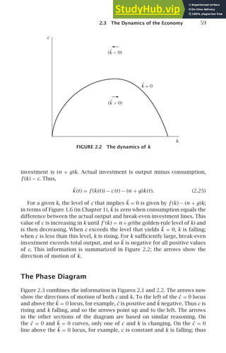
Qualitative Effects
Since the evolution of k is determined by technology rather than prefer-
ences, ρ enters the equation for ċ but not the one for ˙
k. Thus only the ċ = 0
locus is affected. Recall equation (2.24): ċ (t)/c (t) = [f ′
(k (t)) − ρ − θg]/θ.
Thus the value of k where ċ equals zero is defined by f ′
(k∗) = ρ + θg. Since
f ′′
(•) is negative, this means that the fall in ρ raises k∗. Thus the ċ = 0 line
shifts to the right. This is shown in Figure 2.6.
At the time of the change in ρ, the value of k—the stock of capital per unit
of effective labor—is given by the history of the economy, and it cannot
change discontinuously. In particular, k at the time of the change equals
the value of k∗ on the old balanced growth path. In contrast, c—the rate at
which households are consuming—can jump at the time of the shock.
Given our analysis of the dynamics of the economy, it is clear what occurs:
at the instant of the change, c jumps down so that the economy is on the
new saddle path (Point A in Figure 2.6).15
Thereafter, c and k rise gradually
to their new balanced-growth-path values; these are higher than their values
on the original balanced growth path.
Thus the effects of a fall in the discount rate are similar to the effects of
a rise in the saving rate in the Solow model with a capital stock below the
14
See Section 2.7 and Problems 2.11 and 2.12 for examples of how to analyze anticipated
changes.
15
Since we are assuming that the change is unexpected, the discontinuous change in c
does not imply that households are not optimizing. Their original behavior is optimal given
their beliefs; the fall in c is the optimal response to the new information that ρ is lower.](https://image.slidesharecdn.com/advanced-macroeconomics-230806183016-1212def2/85/Advanced-Macroeconomics-88-320.jpg)
![2.6 The Effects of a Fall in the Discount Rate 67
E
A
E′
c
k
k∗
NEW
k∗
OLD
c
.
= 0
= 0
k
.
FIGURE 2.6 The effects of a fall in the discount rate
golden-rule level. In both cases, k rises gradually to a new higher level, and
in both c initially falls but then rises to a level above the one it started at.
Thus, just as with a permanent rise in the saving rate in the Solow model,
the permanent fall in the discount rate produces temporary increases in
the growth rates of capital per worker and output per worker. The only
difference between the two experiments is that, in the case of the fall in ρ,
in general the fraction of output that is saved is not constant during the
adjustment process.
The Rate of Adjustment and the Slope of the Saddle
Path
Equations (2.24) and (2.25) describe ċ (t) and ˙
k (t) as functions of k (t) and
c (t). A fruitful way to analyze their quantitative implications for the dy-
namics of the economy is to replace these nonlinear equations with linear
approximations around the balanced growth path. Thus we begin by taking
first-order Taylor approximations to (2.24) and (2.25) around k = k∗, c = c∗.
That is, we write
ċ ≃
∂ċ
∂k
[k − k∗] +
∂ċ
∂c
[c − c∗], (2.26)
˙
k ≃
∂˙
k
∂k
[k − k∗] +
∂˙
k
∂c
[c − c∗], (2.27)](https://image.slidesharecdn.com/advanced-macroeconomics-230806183016-1212def2/85/Advanced-Macroeconomics-89-320.jpg)
![68 Chapter 2 INFINITE HORIZONS AND OVERLAPPING GENERATIONS
where ∂ċ/∂k, ∂ċ/∂c, ∂˙
k/∂k, and ∂˙
k/∂c are all evaluated at k = k∗, c = c∗. Our
strategy will be to treat (2.26) and (2.27) as exact and analyze the dynamics
of the resulting system.16
It helps to define c̃ = c − c∗ and k̃ = k − k∗. Since c∗ and k∗ are both con-
stant, ˙
c̃ equals ċ, and ˙
k̃ equals ˙
k. We can therefore rewrite (2.26) and (2.27)
as
˙
c̃ ≃
∂ċ
∂k
k̃ +
∂ċ
∂c
c̃, (2.28)
˙
k̃ ≃
∂˙
k
∂k
k̃ +
∂˙
k
∂c
c̃. (2.29)
(Again, the derivatives are all evaluated at k = k∗, c = c∗.) Recall that ċ =
{[f ′
(k) − ρ− θg]/θ}c (equation [2.24]). Using this expression to compute the
derivatives in (2.28) and evaluating them at k = k∗, c = c∗ gives us
˙
c̃ ≃
f ′′
(k∗)c∗
θ
k̃. (2.30)
Similarly, (2.25) states that ˙
k = f (k) − c − (n + g)k. We can use this to find
the derivatives in (2.29); this yields
˙
k̃ ≃ [f ′
(k∗) − (n + g)]k̃ − c̃
= [(ρ + θg) − (n + g)]k̃ − c̃
= βk̃ − c̃,
(2.31)
where the second line uses the fact that (2.24) implies that f ′
(k∗) = ρ + θg
and the third line uses the definition of β as ρ − n − (1 − θ)g. Dividing both
sides of (2.30) by c̃ and both sides of (2.31) by k̃ yields expressions for the
growth rates of c̃ and k̃:
˙
c̃
c̃
≃
f ′′
(k∗)c∗
θ
k̃
c̃
, (2.32)
˙
k̃
k̃
≃ β −
c̃
k̃
. (2.33)
Equations (2.32) and (2.33) imply that the growth rates of c̃ and k̃ depend
only on the ratio of c̃ and k̃. Given this, consider what happens if the values
of c̃ and k̃ are such that c̃ and k̃ are falling at the same rate (that is, if they
imply ˙
c̃/c̃ = ˙
k̃/k̃). This implies that the ratio of c̃ to k̃ is not changing, and
thus that their growth rates are also not changing. That is, if c − c∗ and
16
For a more formal introduction to the analysis of systems of differential equations
(such as [2.26]–[2.27]), see Simon and Blume (1994, Chapter 25).](https://image.slidesharecdn.com/advanced-macroeconomics-230806183016-1212def2/85/Advanced-Macroeconomics-90-320.jpg)
![2.6 The Effects of a Fall in the Discount Rate 69
k − k∗ are initially falling at the same rate, they continue to fall at that rate.
In terms of the diagram, from a point where c̃ and k̃ are falling at equal
rates, the economy moves along a straight line to (k∗,c∗), with the distance
from (k∗,c∗) falling at a constant rate.
Let μ denote ˙
c̃/c̃. Equation (2.32) implies
c̃
k̃
=
f ′′
(k∗)c∗
θ
1
µ
. (2.34)
From (2.33), the condition that ˙
k̃/k̃ equals ˙
c̃/c̃ is thus
µ = β −
f ′′
(k∗)c∗
θ
1
µ
, (2.35)
or
µ2
− βµ +
f ′′
(k∗)c∗
θ
= 0. (2.36)
This is a quadratic equation in µ. The solutions are
µ =
β ± [β2
− 4f ′′
(k∗)c∗/θ]1/2
2
. (2.37)
Let µ1 and µ2 denote these two values of µ.
If µ is positive, then c̃ and k̃ are growing; that is, instead of moving along a
straight line toward (k∗,c∗), the economy is moving on a straight line away
from (k∗,c∗). Thus if the economy is to converge to (k∗,c∗), then µ must
be negative. Inspection of (2.37) shows that only one of the µ’s, namely
{β−[β2
−4f ′′
(k∗)c∗/θ]1/2
}/2, is negative. Let µ1 denote this value of µ. Equa-
tion (2.34) (with µ = µ1) then tells us how c̃ must be related to k̃ for both to
be falling at rate µ1.
Figure 2.7 shows the line along which the economy converges smoothly
to (k∗,c∗); it is labeled AA. This is the saddle path of the linearized system.
The figure also shows the line along which the economy moves directly away
from (k∗,c∗); it is labeled BB. If the initial values of c (0) and k (0) lay along
this line, (2.32) and (2.33) would imply that c̃ and k̃ would grow steadily at
rate µ2.17
Since f ′′
(•) is negative, (2.34) implies that the relation between c̃
and k̃ has the opposite sign from µ. Thus the saddle path AA is positively
sloped, and the BB line is negatively sloped.
Thus if we linearize the equations for ċ and ˙
k, we can characterize the
dynamics of the economy in terms of the model’s parameters. At time 0, c
must equal c∗+ [f ′′
(k∗)c∗/(θµ1)](k−k∗). Thereafter, c and k converge to their
balanced-growth-path values at rate µ1. That is, k (t) = k∗ + eµ1t
[k (0) − k∗]
and c (t) = c∗ + eµ1t
[c (0) − c∗].
17
Of course, it is not possible for the initial value of (k,c) to lie along the BB line. As we
saw in Section 2.3, if it did, either k would eventually become negative or households would
accumulate infinite wealth.](https://image.slidesharecdn.com/advanced-macroeconomics-230806183016-1212def2/85/Advanced-Macroeconomics-91-320.jpg)
![70 Chapter 2 INFINITE HORIZONS AND OVERLAPPING GENERATIONS
B
A
B
E
A
c
k∗ k
= 0
k
.
c
.
= 0
FIGURE 2.7 The linearized phase diagram
The Speed of Adjustment
To understand the implications of (2.37) for the speed of convergence to the
balanced growth path, consider our usual example of Cobb–Douglas pro-
duction, f (k) = kα
. This implies f ′′
(k∗) = α(α− 1)k∗α−2
. Since consumption
on the balanced growth path equals output minus break-even investment,
consumption per unit of effective labor, c∗, equals k∗α
− (n + g)k∗. Thus in
this case we can write the expression for µ1 as
µ1 =
1
2
β − β2
−
4
θ
α(α − 1)k∗α−2
[k∗α
− (n + g)k∗]
1/2
. (2.38)
Recall that on the balanced growth path, f ′
(k) equals ρ + θg (see [2.24]).
For the Cobb–Douglas case, this is equivalent to αk∗α−1
= ρ + θg, or k∗ =
[(ρ + θg)/α]1/(α−1)
. Substituting this into (2.38) and doing some uninterest-
ing algebraic manipulations yields
µ1 =
1
2
β − β2
+
4
θ
1 − α
α
(ρ + θg)[ρ + θg − α(n + g)]
1/2
. (2.39)
Equation (2.39) expresses the rate of adjustment in terms of the underlying
parameters of the model.
To get a feel for the magnitudes involved, suppose α = 1
3
, ρ = 4%, n = 2%,
g = 1%, and θ = 1. One can show that these parameter values imply that on
the balanced growth path, the real interest rate is 5 percent and the saving](https://image.slidesharecdn.com/advanced-macroeconomics-230806183016-1212def2/85/Advanced-Macroeconomics-92-320.jpg)
![2.7 The Effects of Government Purchases 71
rate 20 percent. And since β is defined as ρ−n−(1−θ)g, they imply β = 2%.
Equation (2.38) or (2.39) then implies µ1 ≃ −5.4%. Thus adjustment is quite
rapid in this case; for comparison, the Solow model with the same values
of α, n, and g (and as here, no depreciation) implies an adjustment speed
of 2 percent per year (see equation [1.31]). The reason for the difference is
that in this example, the saving rate is greater than s∗ when k is less than k∗
and less than s∗ when k is greater than k∗. In the Solow model, in contrast,
s is constant by assumption.
2.7 The Effects of Government
Purchases
Thus far, we have left government out of our model. Yet modern economies
devote their resources not just to investment and private consumption but
also to public uses. In the United States, for example, about 20 percent
of total output is purchased by the government; in many other countries
the figure is considerably higher. It is thus natural to extend our model to
include a government sector.
Adding Government to the Model
Assume that the government buys output at rate G(t) per unit of effective
labor per unit time. Government purchases are assumed not to affect util-
ity from private consumption; this can occur if the government devotes the
goods to some activity that does not affect utility at all, or if utility equals
the sum of utility from private consumption and utility from government-
provided goods. Similarly, the purchases are assumed not to affect future
output; that is, they are devoted to public consumption rather than pub-
lic investment. The purchases are financed by lump-sum taxes of amount
G(t) per unit of effective labor per unit time; thus the government always
runs a balanced budget. Consideration of deficit finance is postponed to
Chapter 11. We will see there, however, that in this model the government’s
choice between tax and deficit finance has no impact on any important vari-
ables. Thus the assumption that the purchases are financed with current
taxes only serves to simplify the presentation.
Investment is now the difference between output and the sum of private
consumption and government purchases. Thus the equation of motion for
k, (2.25), becomes
˙
k (t) = f (k (t)) − c (t) − G(t) − (n + g)k (t). (2.40)
A higher value of G shifts the ˙
k = 0 locus down: the more goods that are
purchased by the government, the fewer that can be purchased privately if
k is to be held constant.](https://image.slidesharecdn.com/advanced-macroeconomics-230806183016-1212def2/85/Advanced-Macroeconomics-93-320.jpg)
![72 Chapter 2 INFINITE HORIZONS AND OVERLAPPING GENERATIONS
By assumption, households’ preferences ([2.1]–[2.2] or [2.12]) are un-
changed. Since the Euler equation ([2.20] or [2.24]) is derived from house-
holds’ preferences without imposing their lifetime budget constraint, this
condition continues to hold as before. The taxes that finance the govern-
ment’s purchases affect households’ budget constraint, however. Specifi-
cally, (2.14) becomes
∞
t =0
e−R(t )
c (t)e(n +g)t
dt ≤ k (0) +
∞
t =0
e−R(t )
[w(t) − G(t)]e(n +g)t
dt. (2.41)
Reasoning parallel to that used before shows that this implies the same
expression as before for the limiting behavior of k (equation [2.15]).
The Effects of Permanent and Temporary Changes in
Government Purchases
To see the implications of the model, suppose that the economy is on a
balanced growth path with G(t) constant at some level GL, and that there
is an unexpected, permanent increase in G to GH. From (2.40), the ˙
k = 0
locus shifts down by the amount of the increase in G. Since government
purchases do not affect the Euler equation, the ċ = 0 locus is unaffected.
This is shown in Figure 2.8.18
We know that in response to such a change, c must jump so that the
economy is on its new saddle path. If not, then as before, either capital
would become negative at some point or households would accumulate in-
finite wealth. In this case, the adjustment takes a simple form: c falls by
the amount of the increase in G, and the economy is immediately on its
new balanced growth path. Intuitively, the permanent increases in govern-
ment purchases and taxes reduce households’ lifetime wealth. And because
the increases in purchases and taxes are permanent, there is no scope for
households to raise their utility by adjusting the time pattern of their con-
sumption. Thus the size of the immediate fall in consumption is equal to
the full amount of the increase in government purchases, and the capital
stock and the real interest rate are unaffected.
An older approach to modeling consumption behavior assumes that con-
sumption depends only on current disposable income and that it moves
less than one-for-one with disposable income. Recall, for example, that the
Solow model assumes that consumption is simply fraction 1 − s of current
income. With that approach, consumption falls by less than the amount of
the increase in government purchases. As a result, the rise in government
18
We assume that GH is not so large that k̇ is negative when c = 0. That is, the intersection
of the new k̇ = 0 locus with the ċ = 0 line is assumed to occur at a positive level of c. If it
does not, the government’s policy is not feasible. Even if c is always zero, k̇ is negative, and
eventually the economy’s output per unit of effective labor is less than GH.](https://image.slidesharecdn.com/advanced-macroeconomics-230806183016-1212def2/85/Advanced-Macroeconomics-94-320.jpg)
![2.7 The Effects of Government Purchases 73
E
c
k
E′
= 0
k
.
c
.
= 0
k∗
FIGURE 2.8 The effects of a permanent increase in government purchases
purchases crowds out investment, and so the capital stock starts to fall and
the real interest rate starts to rise. Our analysis shows that those results rest
critically on the assumption that households follow mechanical rules: with
intertemporal optimization, a permanent increase in government purchases
does not cause crowding out.
A more complicated case is provided by an unanticipated increase in G
that is expected to be temporary. For simplicity, assume that the terminal
date is known with certainty. In this case, c does not fall by the full amount
of the increase in G, GH − GL. To see this, note that if it did, consumption
would jump up discontinuously at the time that government purchases re-
turned to GL; thus marginal utility would fall discontinuously. But since the
return of G to GL is anticipated, the discontinuity in marginal utility would
also be anticipated, which cannot be optimal for households.
During the period of time that government purchases are high, ˙
k is gov-
erned by the capital-accumulation equation, (2.40), with G = GH; after G
returns to GL, it is governed by (2.40) with G = GL. The Euler equation,
(2.24), determines the dynamics of c throughout, and c cannot change dis-
continuously at the time that G returns to GL. These facts determine what
happens at the time of the increase in G: c must jump to the value such
that the dynamics implied by (2.40) with G = GH (and by [2.24]) bring the
economy to the old saddle path at the time that G returns to its initial level.
Thereafter, the economy moves along that saddle path to the old balanced
growth path.19
19
As in the previous example, because the initial change in G is unexpected, the discon-
tinuities in consumption and marginal utility at that point do not mean that households are
not behaving optimally. See n. 15.](https://image.slidesharecdn.com/advanced-macroeconomics-230806183016-1212def2/85/Advanced-Macroeconomics-95-320.jpg)
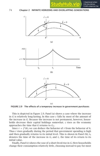
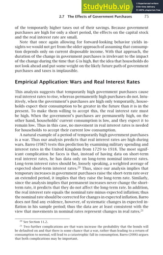


![78 Chapter 2 INFINITE HORIZONS AND OVERLAPPING GENERATIONS
Lt individuals are born in period t. As before, population grows at rate
n; thus Lt = (1 + n)Lt−1. Since individuals live for two periods, at time t
there are Lt individuals in the first period of their lives and Lt−1 = Lt/(1+n)
individuals in their second periods. Each individual supplies 1 unit of labor
when he or she is young and divides the resulting labor income between
first-period consumption and saving. In the second period, the individual
simply consumes the saving and any interest he or she earns.
Let C1t and C2t denote the consumption in period t of young and old
individuals. Thus the utility of an individual born at t, denoted Ut, depends
on C1t and C2t+1. We again assume constant-relative-risk-aversion utility:
Ut =
C1−θ
1t
1 − θ
+
1
1 + ρ
C1−θ
2t +1
1 − θ
, θ 0, ρ −1. (2.43)
As before, this functional form is needed for balanced growth. Because life-
times are finite, we no longer have to assume ρ n + (1 − θ)g to ensure
that lifetime utility does not diverge. If ρ 0, individuals place greater
weight on first-period than second-period consumption; if ρ 0, the situa-
tion is reversed. The assumption ρ −1 ensures that the weight on second-
period consumption is positive.
Production is described by the same assumptions as before. There are
many firms, each with the production function Yt = F (Kt,At Lt). F (•) again
has constant returns to scale and satisfies the Inada conditions, and A again
grows at exogenous rate g (so At = [1 + g]At−1). Markets are competitive;
thus labor and capital earn their marginal products, and firms earn zero
profits. As in the first part of the chapter, there is no depreciation. The real
interest rate and the wage per unit of effective labor are therefore given as
before by rt = f ′
(kt) and wt = f (kt) − ktf ′
(kt). Finally, there is some strictly
positive initial capital stock, K0, that is owned equally by all old individuals.
Thus, in period 0 the capital owned by the old and the labor supplied by
the young are combined to produce output. Capital and labor are paid their
marginal products. The old consume both their capital income and their ex-
isting wealth; they then die and exit the model. The young divide their labor
income, wtAt, between consumption and saving. They carry their saving for-
ward to the next period; thus the capital stock in period t + 1, Kt +1, equals
the number of young individuals in period t, Lt, times each of these individ-
uals’ saving, wtAt − C1t. This capital is combined with the labor supplied by
the next generation of young individuals, and the process continues.
2.9 Household Behavior
The second-period consumption of an individual born at t is
C2t +1 = (1 + rt +1)(wtAt − C1t). (2.44)](https://image.slidesharecdn.com/advanced-macroeconomics-230806183016-1212def2/85/Advanced-Macroeconomics-100-320.jpg)
![2.9 Household Behavior 79
Dividing both sides of this expression by 1 + rt +1 and bringing C1t over to
the left-hand side yields the individual’s budget constraint:
C1t +
1
1 + rt +1
C2t +1 = Atwt. (2.45)
This condition states that the present value of lifetime consumption equals
initial wealth (which is zero) plus the present value of lifetime labor income
(which is Atwt).
The individual maximizes utility, (2.43), subject to the budget constraint,
(2.45). We will consider two ways of solving this maximization problem. The
first is to proceed along the lines of the intuitive derivation of the Euler equa-
tion for the Ramsey model in (2.22)–(2.23). Because the Diamond model is
in discrete time, the intuitive derivation of the Euler equation is much easier
here than in the Ramsey model. Specifically, imagine the individual decreas-
ing C1t by a small (formally, infinitesimal) amount C and then using the ad-
ditional saving and capital income to raise C2t +1 by (1+rt +1)C. This change
does not affect the present value of the individual’s lifetime consumption
stream. Thus if the individual is optimizing, the utility cost and benefit of
the change must be equal. If the cost is less than the benefit, the individual
can increase lifetime utility by making the change. And if the cost exceeds
the benefit, the individual can increase utility by making the reverse change.
The marginal contributions of C1t and C2t +1 to lifetime utility are C −θ
1t
and [1/(1 + ρ)]C−θ
2t +1, respectively. Thus as we let C approach 0, the utility
cost of the change approaches C−θ
1t C and the utility benefit approaches
[1/(1 + ρ)]C−θ
2t +1(1 + rt +1) C. As just described, these are equal when the
individual is optimizing. Thus optimization requires
C−θ
1t C =
1
1 + ρ
C−θ
2t +1(1 + rt +1) C. (2.46)
Canceling the C’s and multiplying both sides by Cθ
2t +1 gives us
Cθ
2t +1
Cθ
1t
=
1 + rt +1
1 + ρ
, (2.47)
or
C2t +1
C1t
=
1 + rt +1
1 + ρ
1/θ
. (2.48)
This condition and the budget constraint describe the individual’s behavior.
Expression (2.48) is analogous to equation (2.21) in the Ramsey model. It
implies that whether an individual’s consumption is increasing or decreas-
ing over time depends on whether the real rate of return is greater or less
than the discount rate. θ again determines how much individuals’ consump-
tion varies in response to differences between r and ρ.](https://image.slidesharecdn.com/advanced-macroeconomics-230806183016-1212def2/85/Advanced-Macroeconomics-101-320.jpg)
![80 Chapter 2 INFINITE HORIZONS AND OVERLAPPING GENERATIONS
The second way to solve the individual’s maximization problem is to set
up the Lagrangian:
L =
C1−θ
1t
1 − θ
+
1
1 + ρ
C1−θ
2t +1
1 − θ
+ λ
Atwt − C1t +
1
1 + rt +1
C2t +1
. (2.49)
The first-order conditions for C1t and C2t +1 are
C−θ
1t = λ, (2.50)
1
1 + ρ
C−θ
2t +1 =
1
1 + rt +1
λ. (2.51)
Substituting the first equation into the second yields
1
1 + ρ
C−θ
2t +1 =
1
1 + rt +1
C−θ
1t . (2.52)
This can be rearranged to obtain (2.48). As before, this condition and the
budget constraint characterize utility-maximizing behavior.
We can use the Euler equation, (2.48), and the budget constraint, (2.45), to
express C1t in terms of labor income and the real interest rate. Specifically,
multiplying both sides of (2.48) by C1t and substituting into (2.45) gives
C1t +
(1 + rt +1)(1−θ)/θ
(1 + ρ)1/θ
C1t = Atwt. (2.53)
This implies
C1t =
(1 + ρ)1/θ
(1 + ρ)1/θ
+ (1 + rt +1)(1−θ)/θ
Atwt. (2.54)
Equation (2.54) shows that the interest rate determines the fraction of
income the individual consumes in the first period. If we let s(r) denote the
fraction of income saved, (2.54) implies
s(r) =
(1 + r)(1−θ)/θ
(1 + ρ)1/θ
+ (1 + r)(1−θ)/θ
. (2.55)
We can therefore rewrite (2.54) as
C1t = [1 − s(rt +1)]Atwt. (2.56)
Equation (2.55) implies that young individuals’ saving is increasing in r
if and only if (1 + r)(1−θ)/θ
is increasing in r. The derivative of (1 + r)(1−θ)/θ
with respect to r is [(1 − θ)/θ](1 + r)(1−2θ)/θ
. Thus s is increasing in r if θ
is less than 1, and decreasing if θ is greater than 1. Intuitively, a rise in
r has both an income and a substitution effect. The fact that the tradeoff
between consumption in the two periods has become more favorable for
second-period consumption tends to increase saving (the substitution ef-
fect), but the fact that a given amount of saving yields more second-period
consumption tends to decrease saving (the income effect). When individuals](https://image.slidesharecdn.com/advanced-macroeconomics-230806183016-1212def2/85/Advanced-Macroeconomics-102-320.jpg)
![2.10 The Dynamics of the Economy 81
are very willing to substitute consumption between the two periods to take
advantage of rate-of-return incentives (that is, when θ is low), the substitu-
tion effect dominates. When individuals have strong preferences for similar
levels of consumption in the two periods (that is, whenθ is high), the income
effect dominates. And in the special case of θ = 1 (logarithmic utility), the
two effects balance, and young individuals’ saving rate is independent of r.
2.10 The Dynamics of the Economy
The Equation of Motion of k
As in the infinite-horizon model, we can aggregate individuals’ behavior to
characterize the dynamics of the economy. As described above, the capital
stock in period t + 1 is the amount saved by young individuals in period t.
Thus,
Kt +1 = s(rt +1)LtAtwt. (2.57)
Note that because saving in period t depends on labor income that period
and on the return on capital that savers expect the next period, it is w in
period t and r in period t + 1 that enter the expression for the capital stock
in period t + 1.
Dividing both sides of (2.57) by Lt +1At +1 gives us an expression for
Kt +1/(At +1 Lt +1), capital per unit of effective labor:
kt +1 =
1
(1 + n)(1 + g)
s(rt +1)wt. (2.58)
We can then substitute for rt +1 and wt to obtain
kt +1 =
1
(1 + n)(1 + g)
s(f ′
(kt +1))[f (kt) − kt f ′
(kt)]. (2.59)
The Evolution of k
Equation (2.59) implicitly defines kt +1 as a function of kt. (It defines kt +1 only
implicitly because kt +1 appears on the right-hand side as well as the left-
hand side.) It therefore determines how k evolves over time given its initial
value. A value of kt such that kt +1 = kt satisfies (2.59) is a balanced-growth-
path value of k: once k reaches that value, it remains there. We therefore
want to know whether there is a balanced-growth-path value (or values) of
k, and whether k converges to such a value if it does not begin at one.](https://image.slidesharecdn.com/advanced-macroeconomics-230806183016-1212def2/85/Advanced-Macroeconomics-103-320.jpg)
![82 Chapter 2 INFINITE HORIZONS AND OVERLAPPING GENERATIONS
45◦
k2 k1
k1
k2
k0 kt
kt+1
k∗
FIGURE 2.11 The dynamics of k
To answer these questions, we need to describe how kt +1 depends on kt.
Unfortunately, we can say relatively little about this for the general case.
We therefore begin by considering the case of logarithmic utility and Cobb–
Douglas production. With these assumptions, (2.59) takes a particularly sim-
ple form. We then briefly discuss what occurs when these assumptions are
relaxed.
Logarithmic Utility and Cobb–Douglas Production
When θ is 1, the fraction of labor income saved is 1/(2 + ρ) (see equation
[2.55]). And when production is Cobb–Douglas, f (k) is kα
and f ′
(k) is αkα−1
.
Equation (2.59) therefore becomes
kt +1 =
1
(1 + n)(1 + g)
1
2 + ρ
(1 − α)kα
t . (2.60)
Figure 2.11 shows kt +1 as a function of kt. A point where the kt +1 function
intersects the 45-degree line is a point where kt +1 equals kt. In the case we
are considering, kt +1 equals kt at kt = 0; it rises above kt when kt is small; and
it then crosses the 45-degree line and remains below. There is thus a unique
balanced-growth-path level of k (aside from k = 0), which is denoted k∗.
k∗ is globally stable: wherever k starts (other than at 0, which is ruled
out by the assumption that the initial capital stock is strictly positive), it](https://image.slidesharecdn.com/advanced-macroeconomics-230806183016-1212def2/85/Advanced-Macroeconomics-104-320.jpg)
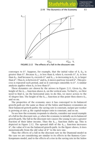
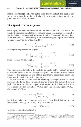
![2.10 The Dynamics of the Economy 85
The convergence to the balanced growth path is determined by λ. If λ is
between 0 and 1, the system converges smoothly. If λ is between −1 and 0,
there are damped oscillations toward k∗: k alternates between being greater
and less than k∗, but each period it gets closer. If λ is greater than 1, the
system explodes. Finally, if λis less than −1, there are explosive oscillations.
To find λ, we return to (2.60): kt +1 = (1−α)kα
t /[(1+n)(1+ g)(2+ρ)]. Thus,
λ ≡
dkt +1
dkt
kt =k∗
= α
1 − α
(1 + n)(1 + g)(2 + ρ)
k∗α−1
= α
1 − α
(1 + n)(1 + g)(2 + ρ)
1 − α
(1 + n)(1 + g)(2 + ρ)
(α−1)/(1−α)
= α,
(2.66)
where the second line uses equation (2.62) to substitute for k∗. That is, λ is
simply α, capital’s share.
Since α is between 0 and 1, this analysis implies that k converges
smoothly to k∗. If α is one-third, for example, k moves two-thirds of the
way toward k∗ each period.25
The rate of convergence in the Diamond model differs from that in the
Solow model (and in a discrete-time version of the Solow model—see Prob-
lem 2.15). The reason is that although the saving of the young is a constant
fraction of their income and their income is a constant fraction of total
income, the dissaving of the old is not a constant fraction of total income.
The dissaving of the old as a fraction of output is Kt/F (Kt ,At Lt), or kt/f (kt).
The fact that there are diminishing returns to capital implies that this ratio
is increasing in k. Since this term enters negatively into saving, it follows
that total saving as a fraction of output is a decreasing function of k. Thus
total saving as a fraction of output is above its balanced-growth-path value
when k k∗, and is below when k k∗. As a result, convergence is more
rapid than in the Solow model.
The General Case
Let us now relax the assumptions of logarithmic utility and Cobb–Douglas
production. It turns out that, despite the simplicity of the model, a wide
range of behaviors of the economy are possible. Rather than attempting a
comprehensive analysis, we merely discuss some of the more interesting
cases.
25
Recall, however, that each period in the model corresponds to half of a person’s
lifetime.](https://image.slidesharecdn.com/advanced-macroeconomics-230806183016-1212def2/85/Advanced-Macroeconomics-107-320.jpg)

![2.10 The Dynamics of the Economy 87
(a)
(d)
(c)
(b)
k∗
1 k∗
3
k∗
1 k∗
2 kt kt
ka kb
k∗
2
kt+1
kt+1
kt
kt
kt+1
kt+1
FIGURE 2.13 Various possibilities for the relationship between kt and kt+1
a low value of kt +1. If saving is sufficiently responsive to r, and if r is suf-
ficiently responsive to k, there can be more than one value of kt +1 that is
consistent with a given kt. Thus the path of the economy is indeterminate:
equation (2.59) (or [2.67]) does not fully determine how k evolves over time
given its initial value. This raises the possibility that self-fulfilling prophecies
and sunspots can affect the behavior of the economy and that the economy
can exhibit fluctuations even though there are no exogenous disturbances.
Depending on precisely what is assumed, various dynamics are possible.26
Thus assuming that there are overlapping generations rather than in-
finitely lived households has potentially important implications for the dy-
namics of the economy: for example, sustained growth may not be possible,
or it may depend on initial conditions.
At the same time, the model does no better than the Solow and Ramsey
models at answering our basic questions about growth. Because of the Inada
26
These issues are briefly discussed further in Section 6.8.](https://image.slidesharecdn.com/advanced-macroeconomics-230806183016-1212def2/85/Advanced-Macroeconomics-109-320.jpg)
![88 Chapter 2 INFINITE HORIZONS AND OVERLAPPING GENERATIONS
conditions, kt +1 must be less than kt for kt sufficiently large. Specifically,
since the saving of the young cannot exceed the economy’s total output,
kt +1 cannot be greater than f (kt)/[(1 + n)(1 + g)]. And because the marginal
product of capital approaches zero as k becomes large, this must eventu-
ally be less than kt. The fact that kt +1 is eventually less than kt implies
that unbounded growth of k is not possible. Thus, once again, growth in
the effectiveness of labor is the only potential source of long-run growth
in output per worker. Because of the possibility of multiple k∗’s, the model
does imply that otherwise identical economies can converge to different bal-
anced growth paths simply because of differences in their initial conditions.
But, as in the Solow and Ramsey models, we can account for quantitatively
large differences in output per worker in this way only by positing immense
differences in capital per worker and in rates of return.
2.11 The Possibility of Dynamic
Inefficiency
The one major difference between the balanced growth paths of the Dia-
mond and Ramsey–Cass–Koopmans models involves welfare. We saw that
the equilibrium of the Ramsey–Cass–Koopmans model maximizes the wel-
fare of the representative household. In the Diamond model, individuals
born at different times attain different levels of utility, and so the appropri-
ate way to evaluate social welfare is not clear. If we specify welfare as some
weighted sum of the utilities of different generations, there is no reason to
expect the decentralized equilibrium to maximize welfare, since the weights
we assign to the different generations are arbitrary.
A minimal criterion for efficiency, however, is that the equilibrium be
Pareto-efficient. It turns out that the equilibrium of the Diamond model
need not satisfy even this standard. In particular, the capital stock on the
balanced growth path of the Diamond model may exceed the golden-rule
level, so that a permanent increase in consumption is possible.
To see this possibility as simply as possible, assume that utility is log-
arithmic, production is Cobb–Douglas, and g is zero. With g = 0, equa-
tion (2.62) for the value of k on the balanced growth path simplifies to
k∗ =
1
1 + n
1
2 + ρ
(1 − α)
1/(1−α)
. (2.68)
Thus the marginal product of capital on the balanced growth path, αk∗α−1
, is
f ′
(k∗) =
α
1 − α
(1 + n)(2 + ρ). (2.69)
The golden-rule capital stock is the capital stock that yields the highest
balanced-growth-path value of the economy’s total consumption per unit of](https://image.slidesharecdn.com/advanced-macroeconomics-230806183016-1212def2/85/Advanced-Macroeconomics-110-320.jpg)
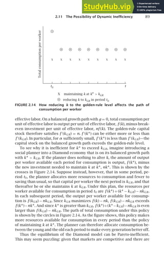

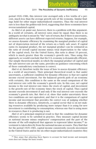
![92 Chapter 2 INFINITE HORIZONS AND OVERLAPPING GENERATIONS
consider. Even in Japan, where investment has been remarkably high, the
profit rate is so great that the returns to capital comfortably exceed invest-
ment. Thus, although decentralized economies can produce dynamically
inefficient outcomes in principle, they do not appear to in practice.
2.12 Government in the Diamond Model
As in the infinite-horizon model, it is natural to ask what happens in the
Diamond model if we introduce a government that makes purchases and
levies taxes. For simplicity, we focus on the case of logarithmic utility and
Cobb–Douglas production.
Let Gt denote the government’s purchases of goods per unit of effective
labor in period t. Assume that it finances those purchases by lump-sum
taxes on the young.
When the government finances its purchases entirely with taxes, workers’
after-tax income in period t is (1 − α)kα
t − Gt rather than (1 − α)kα
t . The
equation of motion for k, equation (2.60), therefore becomes
kt +1 =
1
(1 + n)(1 + g)
1
2 + ρ
[(1 − α)kα
t − Gt ]. (2.70)
A higher Gt therefore reduces kt +1 for a given kt.
To see the effects of government purchases, suppose that the economy
is on a balanced growth path with G constant, and that G increases per-
manently. From (2.70), this shifts the kt +1 function down; this is shown in
Figure 2.15. The downward shift of the kt +1 function reduces k∗. Thus—in
contrast to what occurs in the infinite-horizon model—higher government
purchases lead to a lower capital stock and a higher real interest rate. Intu-
itively, since individuals live for two periods, they reduce their first-period
consumption less than one-for-one with the increase in G. But since taxes
are levied only in the first period of life, this means that their saving falls.
As usual, the economy moves smoothly from the initial balanced growth
path to the new one.
As a second example, consider a temporary increase in government pur-
chases from GL to GH, again with the economy initially on its balanced
growth path. The dynamics of k are thus described by (2.70) with G = GH
during the period that government purchases are high and by (2.70) with
G = GL before and after. That is, the fact that individuals know that gov-
ernment purchases will return to GL does not affect the behavior of the
economy during the time that purchases are high. The saving of the young—
and hence next period’s capital stock—is determined by their after-tax labor
income, which is determined by the current capital stock and by the govern-
ment’s current purchases. Thus during the time that government purchases](https://image.slidesharecdn.com/advanced-macroeconomics-230806183016-1212def2/85/Advanced-Macroeconomics-114-320.jpg)
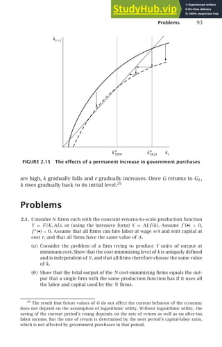
![94 Chapter 2 INFINITE HORIZONS AND OVERLAPPING GENERATIONS
2.2. The elasticity of substitution with constant-relative-risk-aversion utility.
Consider an individual who lives for two periods and whose utility is given
by equation (2.43). Let P1 and P2 denote the prices of consumption in the two
periods, and let W denote the value of the individual’s lifetime income; thus
the budget constraint is P1C1 + P2C2 = W.
(a) What are the individual’s utility-maximizing choices of C1 and C2, given
P1, P2, and W ?
(b) The elasticity of substitution between consumption in the two periods
is −[(P1/P2)/(C1/C2)][∂(C1/C2)/∂(P1/P2)], or −∂ ln (C1/C2)/∂ ln (P1/P2). Show
that with the utility function (2.43), the elasticity of substitution between
C1 and C2 is 1/θ.
2.3. (a) Suppose it is known in advance that at some time t0 the government will
confiscate half of whatever wealth each household holds at that time. Does
consumption change discontinuously at time t0? If so, why (and what is
the condition relating consumption immediately before t0 to consumption
immediately after)? If not, why not?
(b) Suppose it is known in advance that at t0 the government will confiscate
from each household an amount of wealth equal to half of the wealth of
the average household at that time. Does consumption change discontinu-
ously at time t0? If so, why (and what is the condition relating consumption
immediately before t0 to consumption immediately after)? If not, why not?
2.4. Assume that the instantaneous utility function u(C ) in equation (2.1) is
ln C. Consider the problem of a household maximizing (2.1) subject to (2.6).
Find an expression for C at each time as a function of initial wealth plus the
present value of labor income, the path of r(t), and the parameters of the utility
function.
2.5. Consider a household with utility given by (2.1)–(2.2). Assume that the real
interest rate is constant, and let W denote the household’s initial wealth plus
the present value of its lifetime labor income (the right-hand side of [2.6]). Find
the utility-maximizing path of C, given r, W, and the parameters of the utility
function.
2.6. The productivity slowdown and saving. Consider a Ramsey–Cass–Koopmans
economy that is on its balanced growth path, and suppose there is a permanent
fall in g.
(a) How, if at all, does this affect the ˙
k = 0 curve?
(b) How, if at all, does this affect the ċ = 0 curve?
(c) What happens to c at the time of the change?
(d) Find an expression for the impact of a marginal change ing on the fraction
of output that is saved on the balanced growth path. Can one tell whether
this expression is positive or negative?
(e) For the case where the production function is Cobb–Douglas, f (k) = kα
,
rewrite your answer to part (d) in terms of ρ, n, g, θ, and α. (Hint: Use the
fact that f ′
(k∗) = ρ + θg.)](https://image.slidesharecdn.com/advanced-macroeconomics-230806183016-1212def2/85/Advanced-Macroeconomics-116-320.jpg)
![Problems 95
2.7. Describe how each of the following affects the ċ = 0 and ˙
k = 0 curves in
Figure 2.5, and thus how they affect the balanced-growth-path values of c
and k:
(a) A rise in θ.
(b) A downward shift of the production function.
(c) A change in the rate of depreciation from the value of zero assumed in
the text to some positive level.
2.8. Derive an expression analogous to (2.39) for the case of a positive deprecia-
tion rate.
2.9. A closed-form solution of the Ramsey model. (This follows Smith, 2006.)
Consider the Ramsey model with Cobb–Douglas production, y(t) = k (t)α
,
and with the coefficient of relative risk aversion (θ) and capital’s share (α)
assumed to be equal.
(a) What is k on the balanced growth path (k∗)?
(b) What is c on the balanced growth path (c∗)?
(c) Let z(t) denote the capital-output ratio, k (t)/y(t), and x (t) denote the
consumption-capital ratio, c (t)/k(t). Find expressions for ż(t) and ẋ(t)/x(t)
in terms of z, x, and the parameters of the model.
(d) Tentatively conjecture that x is constant along the saddle path. Given this
conjecture:
(i) Find the path of z given its initial value, z(0).
(ii) Find the path of y given the initial value of k, k (0). Is the speed of
convergence to the balanced growth path, d ln[y(t) − y∗]/dt, constant
as the economy moves along the saddle path?
(e) In the conjectured solution, are the equations of motion for c and k, (2.24)
and (2.25), satisfied?
2.10. Capital taxation in the Ramsey–Cass–Koopmans model. Consider a Ramsey–
Cass–Koopmans economy that is on its balanced growth path. Suppose that
at some time, which we will call time 0, the government switches to a policy
of taxing investment income at rate τ. Thus the real interest rate that house-
holds face is now given by r(t) = (1 − τ)f ′
(k (t)). Assume that the government
returns the revenue it collects from this tax through lump-sum transfers.
Finally, assume that this change in tax policy is unanticipated.
(a) How, if at all, does the tax affect the ċ = 0 locus? The ˙
k = 0 locus?
(b) How does the economy respond to the adoption of the tax at time 0? What
are the dynamics after time 0?
(c) How do the values of c and k on the new balanced growth path compare
with their values on the old balanced growth path?
(d) (This is based on Barro, Mankiw, and Sala-i-Martin, 1995.) Suppose there
are many economies like this one. Workers’ preferences are the same in](https://image.slidesharecdn.com/advanced-macroeconomics-230806183016-1212def2/85/Advanced-Macroeconomics-117-320.jpg)
![96 Chapter 2 INFINITE HORIZONS AND OVERLAPPING GENERATIONS
each country, but the tax rates on investment income may vary across
countries. Assume that each country is on its balanced growth path.
(i) Show that the saving rate on the balanced growth path, (y∗ − c∗)/y∗,
is decreasing in τ.
(ii) Do citizens in low-τ, high-k∗, high-saving countries have any incentive
to invest in low-saving countries? Why or why not?
(e) Does your answer to part (c) imply that a policy of subsidizing investment
(that is, making τ 0), and raising the revenue for this subsidy through
lump-sum taxes, increases welfare? Why or why not?
(f ) How, if at all, do the answers to parts (a) and (b) change if the government
does not rebate the revenue from the tax but instead uses it to make
government purchases?
2.11. Using the phase diagram to analyze the impact of an anticipated change.
Consider the policy described in Problem 2.10, but suppose that instead of
announcing and implementing the tax at time 0, the government announces
at time 0 that at some later time, time t1, investment income will begin to be
taxed at rate τ.
(a) Draw the phase diagram showing the dynamics of c and k after time t1.
(b) Can c change discontinuously at time t1? Why or why not?
(c) Draw the phase diagram showing the dynamics of c and k before t1.
(d) In light of your answers to parts (a), (b), and (c), what mustc do at time 0?
(e) Summarize your results by sketching the paths of c and k as functions of
time.
2.12. Using the phase diagram to analyze the impact of unanticipated and antic-
ipated temporary changes. Analyze the following two variations on Problem
2.11:
(a) At time 0, the government announces that it will tax investment income at
rate τ from time 0 until some later date t1; thereafter investment income
will again be untaxed.
(b) At time 0, the government announces that from time t1 to some later
time t2, it will tax investment income at rate τ; before t1 and after t2,
investment income will not be taxed.
2.13. The analysis of government policies in the Ramsey–Cass–Koopmans model
in the text assumes that government purchases do not affect utility from
private consumption. The opposite extreme is that government purchases
and private consumption are perfect substitutes. Specifically, suppose that
the utility function (2.12) is modified to be
U = B
∞
t =0
e−βt [c (t) + G(t)]1−θ
1 − θ
dt.
If the economy is initially on its balanced growth path and if households’
preferences are given by U, what are the effects of a temporary increase in](https://image.slidesharecdn.com/advanced-macroeconomics-230806183016-1212def2/85/Advanced-Macroeconomics-118-320.jpg)
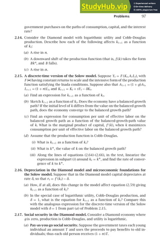
![98 Chapter 2 INFINITE HORIZONS AND OVERLAPPING GENERATIONS
(i) How, if at all, does this change affect equation (2.60) giving kt +1 as a
function of kt?
(ii) How, if at all, does this change affect the balanced-growth-path value
of k?
(iii) If the economy is initially on a balanced growth path that is dynami-
cally efficient, how does a marginal increase in T affect the welfare of
current and future generations? What happens if the initial balanced
growth path is dynamically inefficient?
(b) Fully funded social security. Suppose the government taxes each young
person an amount T and uses the proceeds to purchase capital. Individ-
uals born at t therefore receive (1 + rt +1)T when they are old.
(i) How, if at all, does this change affect equation (2.60) giving kt +1 as a
function of kt?
(ii) How, if at all, does this change affect the balanced-growth-path value
of k?
2.18. The basic overlapping-generations model. (This follows Samuelson, 1958,
and Allais, 1947.) Suppose, as in the Diamond model, that Lt two-period-lived
individuals are born in period t and that Lt = (1 + n)Lt−1. For simplicity, let
utility be logarithmic with no discounting: Ut = ln(C1t) + ln(C2t +1).
The production side of the economy is simpler than in the Diamond
model. Each individual born at time t is endowed with A units of the econ-
omy’s single good. The good can be either consumed or stored. Each unit
stored yields x 0 units of the good in the following period.30
Finally, assume that in the initial period, period 0, in addition to the
L0 young individuals each endowed with A units of the good, there are
[1/(1+n)]L0 individuals who are alive only in period 0. Each of these “old” in-
dividuals is endowed with some amount Z of the good; their utility is simply
their consumption in the initial period, C20.
(a) Describe the decentralized equilibrium of this economy. (Hint: Given the
overlapping-generations structure, will the members of any generation
engage in transactions with members of another generation?)
(b) Consider paths where the fraction of agents’ endowments that is stored,
ft, is constant over time. What is total consumption (that is, consumption
of all the young plus consumption of all the old) per person on such a path
as a function of f ? If x 1 + n, what value of f satisfying 0 ≤ f ≤ 1 max-
imizes consumption per person? Is the decentralized equilibrium Pareto-
efficient in this case? If not, how can a social planner raise welfare?
2.19. Stationary monetary equilibria in the Samuelson overlapping-generations
model. (Again this follows Samuelson, 1958.) Consider the setup described
30
Note that this is the same as the Diamond economy with g = 0, F (Kt,ALt) = ALt + xKt,
and δ = 1. With this production function, since individuals supply 1 unit of labor when they
are young, an individual born in t obtains A units of the good. And each unit saved yields
1 + r = 1 + ∂F (K,AL)/∂K − δ = 1 + x − 1 = x units of second-period consumption.](https://image.slidesharecdn.com/advanced-macroeconomics-230806183016-1212def2/85/Advanced-Macroeconomics-120-320.jpg)
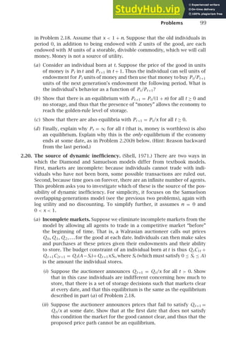


![3.1 Framework and Assumptions 103
Specifics
The model is a simplified version of the models of RD and growth devel-
oped by P. Romer (1990), Grossman and Helpman (1991a), and Aghion and
Howitt (1992).1
The model, like the others we have studied, involves four
variables: labor (L), capital (K ), technology (A), and output (Y ). The model
is set in continuous time. There are two sectors, a goods-producing sector
where output is produced and an RD sector where additions to the stock
of knowledge are made. Fraction aL of the labor force is used in the RD
sector and fraction 1 − aL in the goods-producing sector. Similarly, fraction
aK of the capital stock is used in RD and the rest in goods production. Both
aL and aK are exogenous and constant. Because the use of an idea or a piece
of knowledge in one place does not prevent it from being used elsewhere,
both sectors use the full stock of knowledge, A.
The quantity of output produced at time t is thus
Y(t) = [(1 − aK )K(t)]α
[A(t)(1 − aL)L(t)]1−α
, 0 α 1. (3.1)
Aside from the 1 − aK and 1 − aL terms and the restriction to the Cobb–
Douglas functional form, this production function is identical to those of
our earlier models. Note that equation (3.1) implies constant returns to cap-
ital and labor: with a given technology, doubling the inputs doubles the
amount that can be produced.
The production of new ideas depends on the quantities of capital and
labor engaged in research and on the level of technology. Given our as-
sumption of generalized Cobb–Douglas production, we therefore write
Ȧ(t) = B[aK K(t)]β
[aL L(t)]γ
A(t)θ
, B 0, β ≥ 0, γ ≥ 0, (3.2)
where B is a shift parameter.
Notice that the production function for knowledge is not assumed to
have constant returns to scale to capital and labor. The standard argument
that there must be at least constant returns is a replication one: if the in-
puts double, the new inputs can do exactly what the old ones were doing,
thereby doubling the amount produced. But in the case of knowledge pro-
duction, exactly replicating what the existing inputs were doing would cause
the same set of discoveries to be made twice, thereby leaving Ȧ unchanged.
Thus it is possible that there are diminishing returns in RD. At the same
time, interactions among researchers, fixed setup costs, and so on may be
important enough in RD that doubling capital and labor more than doubles
output. We therefore also allow for the possibility of increasing returns.
The parameter θ reflects the effect of the existing stock of knowledge on
the success of RD. This effect can operate in either direction. On the one
hand, past discoveries may provide ideas and tools that make future
1
See also Uzawa (1965), Shell (1966, 1967), and Phelps (1966b).](https://image.slidesharecdn.com/advanced-macroeconomics-230806183016-1212def2/85/Advanced-Macroeconomics-125-320.jpg)
![104 Chapter 3 ENDOGENOUS GROWTH
discoveries easier. In this case, θ is positive. On the other hand, the eas-
iest discoveries may be made first. In this case, it is harder to make new
discoveries when the stock of knowledge is greater, and so θ is negative.
Because of these conflicting effects, no restriction is placed on θ in (3.2).
As in the Solow model, the saving rate is exogenous and constant. In
addition, depreciation is set to zero for simplicity. Thus,
K̇(t) = sY(t). (3.3)
Likewise, we continue to treat population growth as exogenous and con-
stant. For simplicity, we do not consider the possibility that it is negative.
This implies
L̇(t) = nL(t), n ≥ 0. (3.4)
Finally, as in our earlier models, the initial levels of A, K, and L are given
and strictly positive. This completes the description of the model.2
Because the model has two state variables whose behavior is endogenous,
K and A, it is more complicated to analyze than the Solow model. We there-
fore begin by considering the model without capital; that is, we set α and
β to zero. This case shows most of the model’s central messages. We then
turn to the general case.
3.2 The Model without Capital
The Dynamics of Knowledge Accumulation
When there is no capital in the model, the production function for output
(equation [3.1]) becomes
Y(t) = A(t)(1 − aL)L(t). (3.5)
Similarly, the production function for new knowledge (equation [3.2]) is now
Ȧ(t) = B[aL L(t)]γ
A(t)θ
. (3.6)
Population growth continues to be described by equation (3.4).
Equation (3.5) implies that output per worker is proportional to A, and
thus that the growth rate of output per worker equals the growth rate of
A. We therefore focus on the dynamics of A, which are given by (3.6). This
equation implies that the growth rate of A, denoted gA , is
gA (t) ≡
Ȧ(t)
A(t)
= Ba
γ
L L(t)γ
A(t)θ−1
.
(3.7)
2
The model contains the Solow model with Cobb–Douglas production as a special case:
if β, γ , aK , and aL are all 0 and θ is 1, the production function for knowledge becomes
Ȧ = BA (which implies that A grows at a constant rate), and the other equations of the
model simplify to the corresponding equations of the Solow model.](https://image.slidesharecdn.com/advanced-macroeconomics-230806183016-1212def2/85/Advanced-Macroeconomics-126-320.jpg)
![3.2 The Model without Capital 105
0
gA
gA
∗
.
gA
FIGURE 3.1 The dynamics of the growth rate of knowledge when θ 1
Taking logs of both sides of (3.7) and differentiating the two sides with
respect to time gives us an expression for the growth rate of gA (that is, for
the growth rate of the growth rate of A):
ġA (t)
gA (t)
= γ n + (θ− 1)gA (t). (3.8)
Multiplying both sides of this expression by gA (t) yields
ġA (t) = γ ngA (t) + (θ− 1)[gA (t)]2
. (3.9)
The initial values of L and A and the parameters of the model determine the
initial value of gA (by [3.7]). Equation (3.9) then determines the subsequent
behavior of gA .
To describe further how the growth rate of A behaves (and thus to char-
acterize the behavior of output per worker), we must distinguish among the
cases θ 1, θ 1, and θ = 1. We discuss each in turn.
Case 1: θ 1
Figure 3.1 shows the phase diagram for gA when θ is less than 1. That is, it
plots ġA as a function of A for this case. Because the production function for
knowledge, (3.6), implies that gA is always positive, the diagram considers
only positive values of gA . As the diagram shows, equation (3.9) implies
that for the case of θ less than 1, ġA is positive for small positive values
of gA and negative for large values. We will use g∗
A to denote the unique
positive value of gA that implies that ġA is zero. From (3.9), g∗
A is defined by
γ n + (θ− 1)g∗
A = 0. Solving this for g∗
A yields
g∗
A =
γ
1 − θ
n. (3.10)](https://image.slidesharecdn.com/advanced-macroeconomics-230806183016-1212def2/85/Advanced-Macroeconomics-127-320.jpg)
![106 Chapter 3 ENDOGENOUS GROWTH
0
gA
.
gA
gA
∗
FIGURE 3.2 The effects of an increase in aL when θ 1
This analysis implies that regardless of the economy’s initial conditions,
gA converges to g∗
A . If the parameter values and the initial values of L and A
imply gA (0) g∗
A , for example, ġA is positive; that is, gA is rising. It continues
to rise until it reaches g∗
A . Similarly, if gA (0) g∗
A , then gA falls until it
reaches g∗
A . Once gA reaches g∗
A , both A and Y/L grow steadily at rate g∗
A .
Thus the economy is on a balanced growth path.
This model is our first example of a model of endogenous growth. In this
model, in contrast to the Solow, Ramsey, and Diamond models, the long-run
growth rate of output per worker is determined within the model rather than
by an exogenous rate of technological progress.
The model implies that the long-run growth rate of output per worker,
g∗
A , is an increasing function of the rate of population growth, n. Indeed,
positive population growth is necessary for sustained growth of output per
worker. This may seem troubling; for example, the growth rate of output
per worker is not on average higher in countries with faster population
growth. We will return to this issue after we consider the other cases of the
model.
Equation (3.10) also implies that the fraction of the labor force engaged
in RD does not affect long-run growth. This too may seem surprising: since
growth is driven by technological progress and technological progress is en-
dogenous, it is natural to expect an increase in the fraction of the economy’s
resources devoted to technological progress to increase long-run growth. To
see why it does not, suppose there is a permanent increase in aL starting
from a situation where A is growing at rate g∗
A . This change is analyzed
in Figure 3.2. aL does not enter expression (3.9) for ġA : ġA (t) = γ ngA (t) +
(θ − 1)[ġA (t)]2
. Thus the rise in aL does not affect the curve showing ġA
as a function of gA . But aL does enter expression (3.7) for gA : gA (t) =
Ba
γ
L L(t)
γ
A(t)θ−1
. The increase in aL therefore causes an immediate increase](https://image.slidesharecdn.com/advanced-macroeconomics-230806183016-1212def2/85/Advanced-Macroeconomics-128-320.jpg)
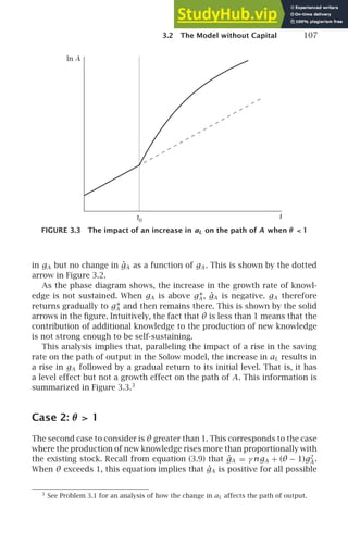

![3.2 The Model without Capital 109
If population growth is positive, gA is growing over time; in this case
the dynamics of the model are similar to those when θ 1.4
If population
growth is zero, on the other hand, gA is constant regardless of the initial
situation. Thus there is no adjustment toward a balanced growth path: no
matter where it begins, the economy immediately exhibits steady growth.
As equations (3.5) and (3.11) show, the growth rates of knowledge, output,
and output per worker are all equal to Ba
γ
L Lγ
in this case. Thus changes in
aL affect the long-run growth rate of the economy.
Since the output good in this economy has no use other than in consump-
tion, it is natural to think of it as being entirely consumed. Thus 1 − aL is
the fraction of society’s resources devoted to producing goods for current
consumption, and aL is the fraction devoted to producing a good (namely,
knowledge) that is useful for producing output in the future. Thus one can
think of aL as a measure of the saving rate in this economy.
With this interpretation, the case of θ = 1 and n = 0 provides a simple
example of a model where the saving rate affects long-run growth. Models of
this form are known as linear growth models; for reasons that will become
clear in Section 3.4, they are also known as Y = AK models. Because of their
simplicity, linear growth models have received a great deal of attention in
work on endogenous growth.
The Importance of Returns to Scale to Produced
Factors
The reason that the three cases have such different implications is that
whether θ is less than, greater than, or equal to 1 determines whether there
are decreasing, increasing, or constant returns to scale to produced factors
of production. The growth of labor is exogenous, and we have eliminated
capital from the model; thus knowledge is the only produced factor. There
are constant returns to knowledge in goods production. Thus whether there
are on the whole increasing, decreasing, or constant returns to knowledge in
this economy is determined by the returns to scale to knowledge in knowl-
edge production—that is, by θ.
4
In the cases of θ 1 and of θ = 1 and n 0, the model implies not merely that growth
is increasing, but that it rises so fast that output reaches infinity in a finite amount of time.
Consider, for example, the case of θ 1 with n = 0. One can check that A(t) = c1/(c2−t)1/(θ−1)
,
with c1 = 1/[(θ − 1)Ba
γ
L Lγ
]1/(θ−1)
and c2 chosen so that A(0) equals the initial value of A,
satisfies (3.6). Thus A explodes at time c2. Since output cannot reach infinity in a finite
time, this implies that the model must break down at some point. But it does not mean that
it cannot provide a good description over the relevant range. Indeed, Section 3.7 presents
evidence that a model similar to this one provides a good approximation to historical data
over many thousands of years.](https://image.slidesharecdn.com/advanced-macroeconomics-230806183016-1212def2/85/Advanced-Macroeconomics-131-320.jpg)

![3.3 The General Case 111
growth raises worldwide income growth. This implication is plausible: be-
cause people are an essential input into producing knowledge, it makes
sense that, at least up to the point where resource limitations (which are
omitted from the model) become important, higher population growth is
beneficial to the growth of worldwide knowledge.
3.3 The General Case
We now want to reintroduce capital into the model and determine how this
modifies the earlier analysis. Thus the model is now described by equations
(3.1)–(3.4) rather than by (3.4)–(3.6).
The Dynamics of Knowledge and Capital
As mentioned above, when the model includes capital, there are two endoge-
nous state variables, A and K. Paralleling our analysis of the simple model,
we focus on the dynamics of the growth rates of A and K. Substituting
the production function, (3.1), into the expression for capital accumulation,
(3.3), yields
K̇(t) = s(1 − aK )α
(1 − aL)1−α
K(t)α
A(t)1−α
L(t)1−α
. (3.13)
Dividing both sides by K(t) and defining cK = s(1 − aK )α
(1 − aL)1−α
gives us
gK (t) ≡
K̇(t)
K(t)
= cK
A(t)L(t)
K(t)
1−α
.
(3.14)
Taking logs of both sides and differentiating with respect to time yields
ġK (t)
gK (t)
= (1 − α)[gA (t) + n − gK (t)]. (3.15)
From (3.13), gK is always positive. Thus gK is rising if gA + n − gK is positive,
falling if this expression is negative, and constant if it is zero. This informa-
tion is summarized in Figure 3.5. In (gA ,gK ) space, the locus of points where
gK is constant has an intercept of n and a slope of 1. Above the locus, gK is
falling; below the locus, it is rising.
Similarly, dividing both sides of equation (3.2), Ȧ = B(aK K)β
(aL L)γ
Aθ
, by
A yields an expression for the growth rate of A:
gA (t) = cA K(t)β
L(t)γ
A(t)θ−1
, (3.16)
where cA ≡ Ba
β
K a
γ
L . Aside from the presence of the Kβ
term, this is essen-
tially the same as equation (3.7) in the simple version of the model. Taking](https://image.slidesharecdn.com/advanced-macroeconomics-230806183016-1212def2/85/Advanced-Macroeconomics-133-320.jpg)
![112 Chapter 3 ENDOGENOUS GROWTH
n
0
gA
gK
.
(gK 0)
.
(gK 0)
.
gK = 0
FIGURE 3.5 The dynamics of the growth rate of capital in the general version
of the model
logs and differentiating with respect to time gives
ġA (t)
gA (t)
= βgK (t) + γ n + (θ − 1)gA (t). (3.17)
Thus gA is rising if βgK + γ n + (θ − 1)gA is positive, falling if it is negative,
and constant if it is zero. This is shown in Figure 3.6. The set of points where
gA is constant has an intercept of −γ n/β and a slope of (1 − θ)/β.5
Above
this locus, gA is rising; and below the locus, it is falling.
The production function for output (equation [3.1]) exhibits constant re-
turns to scale in the two produced factors of production, capital and knowl-
edge. Thus whether there are on net increasing, decreasing, or constant
returns to scale to the produced factors depends on their returns to scale
in the production function for knowledge, equation (3.2). As that equation
shows, the degree of returns to scale to K and A in knowledge produc-
tion is β + θ: increasing both K and A by a factor of X increases Ȧ by
a factor of Xβ+θ
. Thus the key determinant of the economy’s behavior is
now not how θ compares with 1, but how β + θ compares with 1. We will
limit our attention to the cases of β + θ 1 and of β + θ = 1 with n = 0.
The remaining cases (β + θ 1 and β + θ = 1 with n 0) have implica-
tions similar to those of θ 1 in the simple model; they are considered in
Problem 3.6.
5
The figure is drawn for the case of θ 1, so the slope is shown as positive.](https://image.slidesharecdn.com/advanced-macroeconomics-230806183016-1212def2/85/Advanced-Macroeconomics-134-320.jpg)
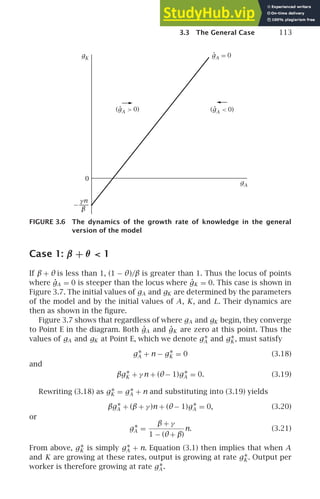
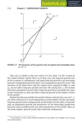
![3.3 The General Case 115
45∘
.
gA = 0
.
gK =
gA
gK
FIGURE 3.8 The dynamics of the growth rates of capital and knowledge when
β + θ = 1 and n = 0
Case 2: β + θ = 1 and n = 0
We have seen that the locus of points where ġK = 0 is given by gK = gA + n,
and that the locus of points where ġA = 0 is given by gK = − (γ n/β) +
[(1 − θ)/β]gA . When β+ θ is 1 and n is 0, both expressions simplify to
gK = gA . That is, in this case the two loci lie directly on top of each other:
both are given by the 45-degree line. Figure 3.8 shows the dynamics of the
economy in this case.
As the figure shows, regardless of where the economy begins, the dynam-
ics of gA and gK carry them to the 45-degree line. Once that happens, gA
and gK are constant, and the economy is on a balanced growth path. As in
the case of θ = 1 and n = 0 in the model without capital, the phase diagram
does not tell us what balanced growth path the economy converges to. One
can show, however, that the economy has a unique balanced growth path for
a given set of parameter values, and that the economy’s growth rate on that
path is a complicated function of the parameters. Increases in the saving rate
and in the size of the population increase this long-run growth rate; the in-
tuition is essentially the same as the intuition for why increases in aL and L
increase long-run growth when there is no capital. And because changes in
aL and aK involve shifts of resources between goods production (and hence
investment) and RD, they have ambiguous effects on long-run growth. Un-
fortunately, the derivation of the long-run growth rate is tedious and not
particularly insightful. Thus we will not work through the details.7
Because
7
See Problem 3.5.](https://image.slidesharecdn.com/advanced-macroeconomics-230806183016-1212def2/85/Advanced-Macroeconomics-137-320.jpg)


![3.4 Knowledge and the Allocation of Resources to RD 119
idea and as licensing its use to the producers of final goods. The fee that
the innovator can charge for the use of the idea is limited by the usefulness
of the idea in production, or by the possibility that others, motivated by
the prospect of high returns, will devote resources to learning the idea. The
quantities of the factors of production engaged in RD are modeled in turn
as resulting from factor movements that equate the private factor payments
in RD with the factor payments in the production of final goods.
Since economies like these are not perfectly competitive, their equilib-
ria are not in general optimal. In particular, the decentralized equilibria
may have inefficient divisions of resources between RD and conventional
goods production. There are in fact three distinct externalities from RD:
the consumer-surplus effect, the business-stealing effect, and the RD effect.
The consumer-surplus effect is that the individuals or firms licensing
ideas from innovators obtain some surplus, since innovators cannot engage
in perfect price discrimination. Thus this is a positive externality from RD.
The business-stealing effect is that the introduction of a superior tech-
nology typically makes existing technologies less attractive, and therefore
harms the owners of those technologies. This externality is negative.9
Finally, the RD effect is that innovators are generally assumed not to
control the use of their knowledge in the production of additional knowl-
edge. In terms of the model of the previous section, innovators are as-
sumed to earn returns on the use of their knowledge in goods production
(equation [3.1]) but not in knowledge production (equation [3.2]). Thus the
development of new knowledge has a positive externality on others engaged
in RD.
The net effect of these three externalities is ambiguous. It is possible to
construct examples where the business-stealing externality outweighs both
the consumer-surplus and RD externalities. In this case the incentives to
capture the profits being earned by other innovators cause too many re-
sources to be devoted to RD. The result is that the economy’s equilibrium
growth rate may be inefficiently high (Aghion and Howitt, 1992). It is gener-
ally believed, however, that the normal situation is for the overall externality
from RD to be positive. In this case the equilibrium level of RD is ineffi-
ciently low, and RD subsidies can increase welfare.
There can be additional externalities as well. For example, if innovators
have only incomplete control over the use of their ideas in goods production
(that is, if there is only partial excludability), there is an additional reason
that the private return to RD is below the social return. On the other hand,
9
Both the consumer-surplus and business-stealing effects are pecuniary externalities:
they operate through markets rather than outside them. As described in Section 2.4, such
externalities do not cause inefficiency in a competitive market. For example, the fact that
an individual’s love of carrots drives up the price of carrots harms other carrot buyers, but
benefits carrot producers. In the competitive case, these harms and benefits balance, and so
the competitive equilibrium is Pareto-efficient. But when there are departures from perfect
competition, pecuniary externalities can cause inefficiency.](https://image.slidesharecdn.com/advanced-macroeconomics-230806183016-1212def2/85/Advanced-Macroeconomics-141-320.jpg)

![3.4 Knowledge and the Allocation of Resources to RD 121
returns as activities whose returns are limited only by the scale of the mar-
ket (creating inventions, for instance). Thus, for example, well-functioning
capital markets that permit firms to expand rapidly tend to promote en-
trepreneurship over rent-seeking. The final factor is the ability to keep the
returns from one’s activities. Thus, clear property rights tend to encourage
entrepreneurship, whereas legally sanctioned rent-seeking (through govern-
ment or religion, for example) tends to encourage socially unproductive
activities.
Learning-by-Doing
The final determinant of knowledge accumulation is somewhat different
in character. The central idea is that, as individuals produce goods, they
inevitably think of ways of improving the production process. For example,
Arrow (1962) cites the empirical regularity that after a new airplane design
is introduced, the time required to build the frame of the marginal aircraft
is inversely proportional to the cube root of the number of aircraft of that
model that have already been produced; this improvement in productivity
occurs without any evident innovations in the production process. Thus
the accumulation of knowledge occurs in part not as a result of deliberate
efforts, but as a side effect of conventional economic activity. This type of
knowledge accumulation is known as learning-by-doing.
When learning-by-doing is the source of technological progress, the rate
of knowledge accumulation depends not on the fraction of the economy’s
resources engaged in RD, but on how much new knowledge is generated
by conventional economic activity. Analyzing learning-by-doing therefore
requires some changes to our model. All inputs are now engaged in goods
production; thus the production function becomes
Y(t) = K(t)α
[A(t)L(t)]1−α
. (3.22)
The simplest case of learning-by-doing is when learning occurs as a side
effect of the production of new capital. With this formulation, since the
increase in knowledge is a function of the increase in capital, the stock of
knowledge is a function of the stock of capital. Thus there is only one state
variable.10
Making our usual choice of a power function, we have
A(t) = BK(t)φ
, B 0, φ 0. (3.23)
Equations (3.22)–(3.23), together with (3.3)–(3.4) describing the accumula-
tion of capital and labor, characterize the economy.
10
See Problem 3.7 for the case in which knowledge accumulation occurs as a side effect
of goods production rather than of capital accumulation.](https://image.slidesharecdn.com/advanced-macroeconomics-230806183016-1212def2/85/Advanced-Macroeconomics-143-320.jpg)
![122 Chapter 3 ENDOGENOUS GROWTH
To analyze this economy, begin by substituting (3.23) into (3.22). This
yields
Y(t) = K(t)α
B1−α
K(t)φ(1−α)
L(t)1−α
. (3.24)
Since K̇(t) = sY(t), the dynamics of K are given by
K̇(t) = sB1−α
K(t)α
K(t)φ(1−α)
L(t)1−α
. (3.25)
In our model of knowledge accumulation without capital in Section 3.2,
the dynamics of A are given by Ȧ(t) = B[aL L(t)]γ
A(t)θ
(equation [3.6]). Com-
paring equation (3.25) of the learning-by-doing model with this equation
shows that the structures of the two models are similar. In the model of Sec-
tion 3.2, there is a single productive input, knowledge. Here, we can think
of there also being only one productive input, capital. As equations (3.6)
and (3.25) show, the dynamics of the two models are essentially the same.
Thus we can use the results of our analysis of the earlier model to analyze
this one. There, the key determinant of the economy’s dynamics is how θ
compares with 1. Here, by analogy, it is how α + φ(1 − α) compares with 1,
which is equivalent to how φ compares with 1.
If φ is less than 1, the long-run growth rate of the economy is a function
of the rate of population growth, n. If φ is greater than 1, there is explosive
growth. And if φ equals 1, there is explosive growth if n is positive and
steady growth if n equals 0.
Once again, a case that has received particular attention is φ = 1 and
n = 0. In this case, the production function (equation [3.24]) becomes
Y(t) = bK(t), b ≡ B1−α
L1−α
. (3.26)
Capital accumulation is therefore given by
K̇(t) = sbK(t). (3.27)
As in the similar cases we have already considered, the dynamics of this
economy are straightforward. Equation (3.27) immediately implies that K
grows steadily at rate sb. And since output is proportional to K, it also grows
at this rate. Thus we have another example of a model in which long-run
growth is endogenous and depends on the saving rate. Moreover, since b is
the inverse of the capital-output ratio, which is easy to measure, the model
makes predictions about the size of the saving rate’s impact on growth—an
issue we will return to in Section 3.6.
In this model, the saving rate affects long-run growth because the con-
tribution of capital is larger than its conventional contribution: increased
capital raises output not only through its direct role in production (the Kα
term in [3.24]), but also by indirectly contributing to the development of new
ideas and thereby making all other capital more productive (the Kφ(1−α)
term
in [3.24]). Because the production function in these models is often written](https://image.slidesharecdn.com/advanced-macroeconomics-230806183016-1212def2/85/Advanced-Macroeconomics-144-320.jpg)

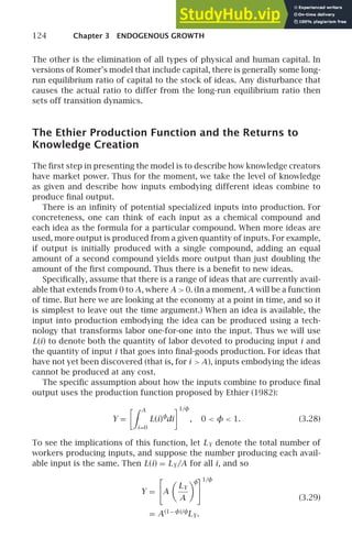
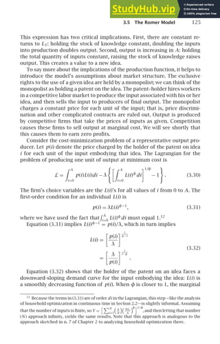
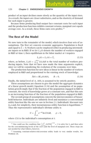
![3.5 The Romer Model 127
As in the Ramsey-Cass-Koopmans model, the individual’s budget con-
straint is that the present value of lifetime consumption cannot exceed his
or her initial wealth plus the present value of lifetime labor income. If indi-
viduals all have the same initial wealth (which we assume) and if the interest
rate is constant (which will prove to be the case in equilibrium), this con-
straint is
∞
t=0
e−rt
C(t)dt ≤ X(0) +
∞
t=0
e−rt
w(t)dt, (3.36)
where r is the interest rate, X(0) is initial wealth per person, and w(t) is the
wage at t. The individual takes all of these as given.
The third set of assumptions concern the microeconomics of RD. There
is free entry into idea creation: anyone can hire 1/[BA(t)] units of labor at
the prevailing wage w(t) and produce a new idea (see [3.34]). Even though
an increase in A raises productivity in RD, RD firms are not required to
compensate the inventors of past ideas. Thus the model assumes the RD
externality discussed in Section 3.4.
The creator of an idea is granted permanent patent rights to the use of
the idea in producing the corresponding input into output production (but,
as just described, not in RD). The patent-holder chooses how much of the
input that embodies his or her idea to produce, and the price to charge for
the input, at each point in time. In making this decision, the patent-holder
takes as given the wage, the prices charged for other inputs, and the total
amount of labor used in goods production, LY.15
The free-entry condition in RD requires that the present value of the
profits earned from selling the input embodying an idea equals the cost
of creating it. Suppose idea i is created at time t, and let π(i,τ) denote the
profits earned by the creator of the idea at time τ. Then this condition is
∞
τ=t
e−r (τ−t )
π(i,τ)dτ =
w(t)
BA(t)
. (3.37)
The final assumptions of the model concern general equilibrium. First,
the assumption that the labor market is competitive implies that the wage
paid in RD and the wages paid by all input producers are equal. Second, the
only asset in the economy is the patents. Thus initial wealth is the present
value of the future profits from the ideas that have already been invented.
Finally, the only use of the output good is for consumption. Because all
15
It might seem natural to assume that the patent-holder takes the price charged by
producers of final goods rather than LY as given. However, this approach implies that no
equilibrium exists. Consider a situation where the price charged by goods producers equals
their marginal cost. If one patent-holder cuts his or her price infinitesimally with the prices
of other inputs and of final output unchanged, goods producers’ marginal cost is less than
price, and so their input demands are infinite. Assuming that patent-holders take LY as given
avoids this problem.](https://image.slidesharecdn.com/advanced-macroeconomics-230806183016-1212def2/85/Advanced-Macroeconomics-149-320.jpg)
![128 Chapter 3 ENDOGENOUS GROWTH
individuals are the same, they all choose the same consumption path. Thus
equilibrium in the goods market at time t requires
C(t)L = Y(t). (3.38)
This completes the description of the model.
Solving the Model
The fact that at the aggregate level the economy resembles a linear growth
model suggests that in equilibrium, the allocation of labor between RD
and the production of intermediate inputs is likely not to change over time.
Thus, rather than taking a general approach to find the equilibrium, we will
look for an equilibrium where LA and LY are constant. Specifically, we will in-
vestigate the implications of a given (and constant) value of LA to the point
where we can find what it implies about both the present value of the profits
from the creation of an idea and the cost of creating the idea. The condition
that these two quantities must be equal will then pin down the equilibrium
value of LA . We will then verify that this equilibrium value is constant over
time.
Of course, this approach will not rule out the possibility that there are
also equilibria where LA varies over time. It turns out, however, that there
are no such equilibria, and thus that the equilibrium we will find is the
model’s only one. We will not demonstrate this formally, however.
The first step in solving the model is to consider the problem of a patent-
holder choosing the price to charge for his or her input at a point in time.
A standard result from microeconomics is that the profit-maximizing price
of a monopolist is η/(η− 1) times marginal cost, where η is the elasticity of
demand. In our case, we know from equation (3.32) for cost-minimization
by the producers of final goods that the elasticity of demand is constant
and equal to 1/(1 − φ). And since one unit of the input can be produced
from one unit of labor, the marginal cost of supplying the input at time t is
w(t). Each monopolist therefore charges [1/(1 − φ)]/{[1/(1 − φ)] − 1} times
w(t), or w(t)/φ.16
Knowing the price each monopolist charges allows us to determine his or
her profits at a point in time. Because the prices of all inputs are the same,
the quantity of each input used at time t is the same. Given our assumption
that LA is constant and the requirement that LA (t)+ LY(t) = L, this quantity
16
This neglects the potential complication that the analysis in equations (3.30)–(3.32)
shows the elasticity of input demand conditional on producing a given amount of output.
Thus we might need to consider possible effects through changes in the quantity of output
produced. However, because each input accounts for an infinitesimal fraction of total costs,
the impact of a change in the price of a single input on the total amount produced from a
given LY is negligible. Thus allowing for the possibility that a change in p(i) could change
the quantity produced does not change the elasticity of demand each monopolist faces.](https://image.slidesharecdn.com/advanced-macroeconomics-230806183016-1212def2/85/Advanced-Macroeconomics-150-320.jpg)
![3.5 The Romer Model 129
is (L − LA )/A(t). Each patent-holder’s profits are thus
π(t) =
L − LA
A(t)
w(t)
φ
− w(t)
(3.39)
=
1 − φ
φ
L − LA
A(t)
w(t).
To determine the present value of profits from an invention, and hence
the incentive to innovate, we need to determine the economy’s growth rate
and the interest rate. Equation (3.34) for knowledge creation, Ȧ(t) =
BLA (t)A(t), implies that if LA is constant, Ȧ(t)/A(t) is just BLA . We know that
all input suppliers charge the same price at a point in time, and thus that
all available inputs are used in the same quantity. Equation (3.29) tells us
that in this case, Y(t) = A(t)[(1−φ)/φ]
LY(t). Since LY(t) is constant, the growth
rate of Y is (1 − φ)/φ times the growth rate of A, or [(1 − φ)/φ]BLA .
Both consumption and the wage grow at the same rate as output. In the
case of consumption, we know this because all output is consumed. In the
case of the wage, one way to see this is to note that because of constant
returns and competition, all the revenues of final goods producers are paid
to the intermediate goods suppliers. Because their markup is constant, their
payments to workers are a constant fraction of their revenues. Since the
number of workers producing intermediate inputs is constant, it follows
that the growth rate of the wage equals the growth rate of output.
We can use this analysis, together with equation (3.39), to find the growth
rate of profits from an invention. L − LA is constant; w is growing at rate
[(1 − φ)/φ]BLA ; and A is growing at rate BLA . Equation (3.39) then implies
that profits from a given invention are growing at rate [(1−φ)/φ]BLA −BLA ,
or [(1 − 2φ)/φ]BLA .
Once we know the growth rate of consumption, finding the real interest
rate is straightforward. Recall from Section 2.2 that consumption growth
for a household with constant-relative-risk-aversion utility is Ċ(t)/C(t) =
[r(t) − ρ]/θ, where θ is the coefficient of relative risk aversion. With loga-
rithmic utility, θ is 1. Thus equilibrium requires
r(t) = ρ +
Ċ(t)
C(t)
(3.40)
= ρ +
1 − φ
φ
BLA .
Thus if LA is constant, the real interest rate is constant, as we have been
assuming.
The profits from an invention grow at rate [(1 − 2φ)/φ]BLA , and are dis-
counted at the interest rate, ρ+ [(1 − φ)/φ]BLA . Equation (3.39) tells us that
the profits at t are [(1 − φ)/φ][(L − LA )w(t)/A(t)]. The present value of the](https://image.slidesharecdn.com/advanced-macroeconomics-230806183016-1212def2/85/Advanced-Macroeconomics-151-320.jpg)
![130 Chapter 3 ENDOGENOUS GROWTH
profits earned from the discovery of a new idea at time t is therefore
π(t) =
1 − φ
φ
(L − LA )
w(t)
A(t)
ρ +
1 − φ
φ
BLA −
1 − 2φ
φ
BLA
(3.41)
=
1 − φ
φ
L − LA
ρ + BLA
w(t)
A(t)
.
We are now in a position to find the equilibrium value of LA . If the amount
of RD is strictly positive, the present value of profits from an invention
must equal the costs of the invention. Since one worker can produce BA(t)
ideas per unit time, the cost of an invention is w(t)/[BA(t)]. The equilibrium
condition is therefore
1 − φ
φ
L − LA
ρ + BLA
w(t)
A(t)
=
w(t)
BA(t)
. (3.42)
Solving this equation for LA yields
LA = (1 − φ)L −
φρ
B
. (3.43)
The amount of RD need not be strictly positive, however. In particular,
when (3.43) implies LA 0, the discounted profits from the first invention
starting from LA = 0 are less than its costs. As a result, RD is 0. Thus we
need to modify equation (3.43) to
LA = max
(1 − φ)L −
φρ
B
,0
. (3.44)
Finally, since the growth rate of output is [(1 − φ)/φ]BLA , we have
Ẏ (t)
Y(t)
= max
(1 − φ)2
φ
BL − (1 − φ)ρ,0
. (3.45)
Thus we have succeeded in describing how long-run growth is determined
by the underlying microeconomic environment. And note that since none of
the terms on the right-hand side of (3.40) are time-varying, the equilibrium
value of LA is constant.17
17
To verify that individuals are satisfying their budget constraint, recall from Sec-
tion 2.2 that the lifetime budget constraint can be expressed in terms of the behavior of
wealth as t approaches infinity. When the interest rate is constant, this version of the bud-
get constraint simplifies to limt→∞ e−rt
[X(t)/L ] ≥ 0. X(t), the economy’s wealth at t, is the
present value of future profits from ideas already invented, and is growing at the growth
rate of the economy. From (3.40), the interest rate exceeds the economy’s growth rate.
Thus limt→∞ e−rt
[X(t)/L ] = 0, and so individuals are satisfying their budget constraint with
equality.](https://image.slidesharecdn.com/advanced-macroeconomics-230806183016-1212def2/85/Advanced-Macroeconomics-152-320.jpg)
![3.5 The Romer Model 131
Implications
The model has two major sets of implications. The first concern the deter-
minants of long-run growth. Four parameters affect the economy’s growth
rate.18
First, when individuals are less patient (that is, when ρ is higher),
fewer workers engage in RD (equation [3.44]), and so growth is lower (equa-
tion [3.45]). Since RD is a form of investment, this makes sense.
Second, an increase in substitutability among inputs (φ) also reduces
growth. There are two reasons. First, fewer workers engage in RD (again,
equation [3.44]). Second, although a given amount of RD translates into the
same growth rate of A (equation [3.34]), a given growth rate of A translates
into slower output growth (equation [3.29]). This finding is also intuitive:
when the inputs embodying different ideas are better substitutes, patent-
holders’ market power is lower, and each additional idea contributes less to
output. Both effects make RD less attractive.
Third, an increase in productivity in the RD sector (B) increases growth.
There are again two effects at work. The first is the straightforward one that
a rise in B raises growth for a given number of workers engaged in RD.
The other is that increased productivity in RD draws more workers into
that sector.
Finally, an increase in the size of the population (L) raises long-run
growth. Paralleling the effects of an increase in B, there are two effects:
growth increases for a given fraction of workers engaged in RD, and the
fraction of workers engaged in RD increases. The second effect is another
consequence of the nonrivalry of knowledge: an increase in the size of the
economy expands the market an inventor can reach, and so increases the
returns to RD.
All four parameters affect growth at least in part by changing the fraction
of workers who are engaged in RD. None of these effects are present in
the simple model of RD and growth in Sections 3.1–3.3, since that model
takes the allocation of workers between activities as given. Thus the Romer
model identifies a rich set of determinants of long-run growth.
The model’s second major set of implications concern the gap between
equilibrium and optimal growth. Since the economy is not perfectly com-
petitive, there is no reason to expect the decentralized equilibrium to be
socially optimal. Paralleling our analysis of the equilibrium, let us look for
the constant level of LA that yields the highest level of lifetime utility for
the representative individual.19
Because all output is consumed, the representative individual’s consump-
tion is 1/L times output. Equation (3.29) for output therefore implies that
18
The discussion that follows assumes that the parameter values are in the range where
LA is strictly positive.
19
One can show that a social planner would in fact choose to have LA be constant, so
the restriction to paths where LA is constant is not a binding constraint.](https://image.slidesharecdn.com/advanced-macroeconomics-230806183016-1212def2/85/Advanced-Macroeconomics-153-320.jpg)
![132 Chapter 3 ENDOGENOUS GROWTH
the representative individual’s consumption at time 0 is
C(0) =
(L − LA )A(0)(1−φ)/φ
L
. (3.46)
Output and consumption grow at rate [(1 − φ)/φ]BLA . The representative
individual’s lifetime utility is therefore
U =
∞
t=0
e−ρt
ln
L − LA
L
A(0)(1−φ)/φ
e[(1−φ)/φ]BLA t
dt. (3.47)
One can show that the solution to this integral is20
U =
1
ρ
ln
L − LA
L
+
1 − φ
φ
ln A(0) +
1 − φ
φ
BLA
ρ
. (3.48)
Maximizing this expression with respect to LA shows that the socially opti-
mal level of LA is given by21
LOPT
A = max
L −
φ
1 − φ
ρ
B
,0
. (3.49)
Comparing this expression with equation (3.44) for the equilibrium level of
LA shows a simple relation between the two:
L
EQ
A = (1 − φ)LOPT
A , (3.50)
where L
EQ
A is the equilibrium level of LA .
The model potentially has all three externalities described in Section 3.4.
There is a consumer-surplus effect (or, in this case, a goods-producer-
surplus effect): because a patent-holder charges a fixed price per unit of the
input embodying his or her idea, the firms producing final output obtain
surplus from buying the intermediate input. There can be either a business-
stealing or a business-creating effect. Equation (3.39) shows that the prof-
its of each supplier of intermediate goods are proportional to w(t)/A(t).
w(t) is proportional to Y(t), which is proportional to A(t)(1−φ)/φ
. Thus prof-
its are proportional to A(t)(1−2φ)/φ
. It follows that the profits of existing
patent-holders are reduced by an increase in A if φ 1/2, but increased
if φ 1/2. Finally, there is an RD effect: an increase in A makes the RD
sector more productive, but innovators do not have to compensate existing
patent-holders for this benefit.
Despite the three externalities, the relation between the equilibrium and
optimal allocation of workers to RD takes a simple form. The equilibrium
number of workers engaged in RD is always less than the optimal num-
ber (unless both are at the corner solution of zero). Thus growth is always
inefficiently low. Moreover, the proportional gap between the equilibrium
20
See Problem 3.10.
21
Again, see Problem 3.10.](https://image.slidesharecdn.com/advanced-macroeconomics-230806183016-1212def2/85/Advanced-Macroeconomics-154-320.jpg)
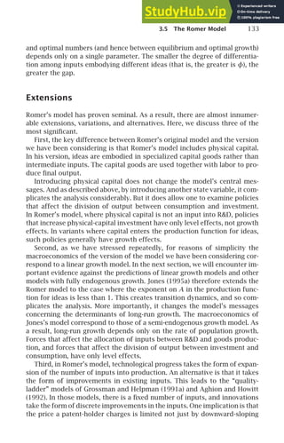

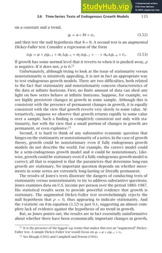
![136 Chapter 3 ENDOGENOUS GROWTH
The two-standard-error confidence interval for b in (3.52) is (−0. 026, 0. 028).
A value of 0.02, which is comfortably within the confidence interval, implies
that annual growth is rising by 0.2 percentage points per decade, and thus
that average growth was more than two percentage points higher at the end
of Jones’s sample than at the beginning. That is, while the results do not
reject the null of no trend in growth, they also fail to reject the null of an
enormous trend in growth.
Intuitively, what the statistical results are telling us is not whether growth
is stationary or nonstationary—which, as just described, is both impossible
and uninteresting. Rather, they are telling us that there are highly transitory
movements in growth that are large relative to any long-lasting movements
that may be present. But this does not tell us whether such long-lasting
movements are economically important.
The Magnitudes and Correlates of Changes in
Long-Run Growth
Jones’s second approach is to examine the relationships between the de-
terminants of growth identified by endogenous growth models and actual
growth rates. He begins by considering learning-by-doing models like the
one discussed in Section 3.4 with φ = 1. Recall that that model yields a
relationship of the form
Y(t)
L(t)
= b
K(t)
L(t)
(3.54)
(see equation [3.26]). This implies that the growth rate of income per per-
son is
gY/L(t) = gK (t) − gL(t), (3.55)
where gx denotes the growth rate of x. gK is given by
K̇(t)
K(t)
=
sY(t)
K(t)
− δ, (3.56)
where s is the fraction of output that is invested and δ is the depreciation
rate.
Jones observes that Y/K, δ, and gL all both appear to be fairly steady,
while investment rates have been trending up. Thus the model predicts an
upward trend in growth. More importantly, it makes predictions about the
magnitude of the trend. Jones reports that in most major industrialized
countries, Y/K is about 0.4 and the ratio of investment to GDP has been ris-
ing by about one percentage point per decade. The model therefore predicts
an increase in growth of about 0.4 percentage points per decade. This figure
is far outside the confidence interval noted above for the estimated trend in](https://image.slidesharecdn.com/advanced-macroeconomics-230806183016-1212def2/85/Advanced-Macroeconomics-158-320.jpg)


![3.7 Population Growth and Technological Change since 1 Million B.C. 139
technological progress fallen to any substantial degree on output per person.
Putting these observations together, Kremer concludes that models of en-
dogenous technological progress predict that over most of human history,
the rate of population growth should have been rising.
A Simple Model
Kremer’s formal model is a straightforward variation on the models we have
been considering. The simplest version consists of three equations. First,
output depends on technology, labor, and land:
Y(t) = Tα
[A(t)L(t)]1−α
, (3.57)
where T denotes the fixed stock of land. (Capital is neglected for simplic-
ity, and land is included to keep population finite.) Second, additions to
knowledge are proportional to population, and also depend on the stock of
knowledge:
Ȧ(t) = BL(t)A(t)θ
. (3.58)
And third, population adjusts so that output per person equals the subsis-
tence level, denoted y:
Y(t)
L(t)
= y. (3.59)
Aside from this Malthusian assumption about the determination of popu-
lation, this model is similar to the model of Section 3.2 with γ = 1.
We solve the model in two steps. The first is to find the size of the pop-
ulation that can be supported on the fixed stock of land at a given time.
Substituting expression (3.57) for output into the Malthusian population
condition, (3.59), yields
Tα
[A(t)L(t)]1−α
L(t)
= y. (3.60)
Solving this condition for L(t) gives us
L(t) =
1
y
1/α
A(t)(1−α)/α
T. (3.61)
This equation states that the population that can be supported is decreas-
ing in the subsistence level of output, increasing in technology, and propor-
tional to the amount of land.
The second step is to find the dynamics of technology and population.
Since both y and T are constant, (3.61) implies that the growth rate of L is
(1 − α)/α times the growth rate of A:
L̇(t)
L(t)
=
1 − α
α
Ȧ(t)
A(t)
. (3.62)](https://image.slidesharecdn.com/advanced-macroeconomics-230806183016-1212def2/85/Advanced-Macroeconomics-161-320.jpg)
![140 Chapter 3 ENDOGENOUS GROWTH
In the special case of θ = 1, equation (3.58) for knowledge accumulation im-
plies that Ȧ(t)/A(t) is just BL(t). Thus in this case, (3.62) implies that the
growth rate of population is proportional to the level of population. In the
general case, one can show that the model implies that the rate of popu-
lation growth is proportional to L(t)ψ
, where ψ = 1 − [(1 − θ)α/(1 − α)].24
Thus population growth is increasing in the size of the population unless α
is large or θ is much less than 1 (or a combination of the two). Intuitively,
Kremer’s model implies increasing growth even with diminishing returns
to knowledge in the production of new knowledge (that is, even with θ 1)
because labor is now a produced factor: improvements in technology lead
to higher population, which in turn leads to further improvements in tech-
nology. Further, the effect is likely to be substantial. For example, even if
α is one-third and θ is one-half rather than 1, 1 − [(1 − θ)α/(1 − α)] is 0.75.
Results
Kremer tests the model’s predictions using population estimates extend-
ing back to 1 million B.C. that have been constructed by archaeologists and
anthropologists. Figure 3.9 shows the resulting scatter plot of population
growth against population. Each observation shows the level of popula-
tion at the beginning of some period and the average annual growth rate
of population over that period. The length of the periods considered falls
gradually from many thousand years early in the sample to 10 years at the
end. Because the periods considered for the early part of the sample are so
long, even substantial errors in the early population estimates would have
little impact on the estimated growth rates.
The figure shows a strongly positive, and approximately linear, relation-
ship between population growth and the level of population. A regression
of growth on a constant and population (in billions) yields
nt = −0.0023
(0.0355)
+ 0.524
(0.026)
Lt, R2
= 0.92, D.W. = 1.10, (3.63)
where n is population growth and L is population, and where the num-
bers in parentheses are standard errors. Thus there is an overwhelmingly
statistically significant association between the level of population and its
growth rate.
The argument that technological progress is a worldwide phenomenon
fails if there are regions that are completely cut off from one another.
Kremer uses this observation to propose a second test of theories of
24
To see this, divide both sides of (3.58) by A to obtain an expression for Ȧ/A. Then
use (3.60) to express A in terms of L, and substitute the result into the expression for Ȧ/A.
Expression (3.62) then implies that L̇/L equals a constant times L(t)ψ
.](https://image.slidesharecdn.com/advanced-macroeconomics-230806183016-1212def2/85/Advanced-Macroeconomics-162-320.jpg)
![3.7 Population Growth and Technological Change since 1 Million B.C. 141
−0.005
0.000
0.005
0.010
0.015
0.020
0.025
Population
growth
rate
0 2 3 4 5
1
Population (billions)
+
+
+
++
+ +
+
+
++
++++
+
+
+
+
+
+
+
+ + +
+
+
+
+
+ +
FIGURE 3.9 The level and growth rate of population, 1 million B.C. to 1990 (from
Kremer, 1993; used with permission)
endogenous knowledge accumulation. From the disappearance of the inter-
continental land bridges at the end of the last ice age to the voyages of the
European explorers, Eurasia-Africa, the Americas, Australia, and Tasmania
were almost completely isolated from one another. The model implies that
at the time of the separation, the populations of each region had the same
technology. Thus the initial populations should have been approximately
proportional to the land areas of the regions (see equation [3.61]). The
model predicts that during the period that the regions were separate, tech-
nological progress was faster in the regions with larger populations. The
theory thus predicts that, when contact between the regions was reestab-
lished around 1500, population density was highest in the largest regions.
Intuitively, inventions that would allow a given area to support more people,
such as the domestication of animals and the development of agriculture,
were much more likely in Eurasia-Africa, with its population of millions,
than in Tasmania, with its population of a few thousand.
The data confirm this prediction. The land areas of the four regions are
84 million square kilometers for Eurasia-Africa, 38 million for the Americas,
8 million for Australia, and 0.1 million for Tasmania. Population estimates
for the four regions in 1500 imply densities of approximately 4.9 people
per square kilometer for Eurasia-Africa, 0.4 for the Americas, and 0.03 for
both Australia and Tasmania.25
25
Kremer argues that, since Australia is largely desert, these figures understate
Australia’s effective population density. He also argues that direct evidence suggests that
Australia was more technologically advanced than Tasmania. Finally, he notes that there
was in fact a fifth separate region, Flinders Island, a 680-square-kilometer island between
Tasmania and Australia. Humans died out entirely on Flinders Island around 3000 B.C.](https://image.slidesharecdn.com/advanced-macroeconomics-230806183016-1212def2/85/Advanced-Macroeconomics-163-320.jpg)
![142 Chapter 3 ENDOGENOUS GROWTH
Discussion
What do we learn from the confirmation of the model’s time-series and
cross-section predictions? The basic source of Kremer’s predictions is the
idea that the rate of increase in the stock of knowledge is increasing in
population: innovations do not arrive exogenously, but are made by people.
Although this idea is assumed away in the Solow, Ramsey, and Diamond
models, it is hardly controversial. Thus Kremer’s main qualitative findings
for the most part confirm predictions that are not at all surprising.
Any tractable model of technological progress and population growth
over many millennia must inevitably be so simplified that it would closely
match the quantitative features of the data only by luck. For example, it
would be foolish to attach much importance to the finding that population
growth appears to be roughly proportional to the level of population rather
than to L0.75
or L0.9
. Thus, Kremer’s evidence tells us little about, say, the
exact value of θ in equation (3.58).
The value of Kremer’s evidence, then, lies not in discriminating among
alternative theories of growth, but in using growth theory to help under-
stand major features of human history. The dynamics of human population
over the very long run and the relative technological performance of differ-
ent regions in the era before 1500 are important issues. Kremer’s evidence
shows that the ideas of new growth theory shed significant light on them.
Population Growth versus Growth in Income per
Person over the Very Long Run
As described above, over nearly all of history technological progress has led
almost entirely to higher population rather than to higher average income.
But this has not been true over the past few centuries: the enormous tech-
nological progress of the modern era has led not only to vast population
growth, but also to vast increases in average income.
It may appear that explaining this change requires appealing to some de-
mographic change, such as the development of contraceptive techniques or
preferences for fewer children when technological progress is rapid. In fact,
however, Kremer shows that the explanation is much simpler. Malthusian
population dynamics are not instantaneous. Rather, at low levels of income,
population growth is an increasing function of income. That is, Kremer ar-
gues that instead of assuming that Y/L always equals y (equation [3.59]),
it is more realistic to assume n = n(y), with n(y) = 0 and n′
(•) 0 in the
vicinity of y.
This formulation implies that when income rises, population growth rises,
tending to push income back down. When technological progress is slow,
the fact that the adjustment is not immediate is of little importance. With](https://image.slidesharecdn.com/advanced-macroeconomics-230806183016-1212def2/85/Advanced-Macroeconomics-164-320.jpg)


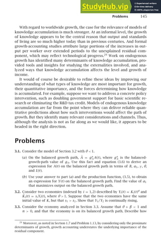
![146 Chapter 3 ENDOGENOUS GROWTH
each of the following changes affects the ġA = 0 and ġK = 0 lines and the
position of the economy in (gA ,gK ) space at the moment of the change:
(a) An increase in n.
(b) An increase in aK .
(c) An increase in θ.
3.4. Consider the economy described in Section 3.3, and assume β + θ 1 and
n 0. Suppose the economy is initially on its balanced growth path, and that
there is a permanent increase in s.
(a) How, if at all, does the change affect the ġA = 0 and ġK = 0 lines? How,
if at all, does it affect the location of the economy in (gA ,gK ) space at the
time of the change?
(b) What are the dynamics of gA and gK after the increase in s? Sketch the
path of log output per worker.
(c) Intuitively, how does the effect of the increase in s compare with its effect
in the Solow model?
3.5. Consider the model of Section 3.3 with β + θ = 1 and n = 0.
(a) Using (3.14) and (3.16), find the value that A/K must have for gK and gA
to be equal.
(b) Using your result in part (a), find the growth rate of A and K when gK = gA .
(c) How does an increase in s affect the long-run growth rate of the economy?
(d) What value of aK maximizes the long-run growth rate of the economy?
Intuitively, why is this value not increasing in β, the importance of capital
in the RD sector?
3.6. Consider the model of Section 3.3 with β + θ 1 and n 0.
(a) Draw the phase diagram for this case.
(b) Show that regardless of the economy’s initial conditions, eventually the
growth rates of A and K (and hence the growth rate of Y ) are increasing
continually.
(c) Repeat parts (a) and (b) for the case of β + θ = 1, n 0.
3.7. Learning-by-doing. Suppose that output is given by equation (3.22), Y (t) =
K(t)α
[A(t)L(t)]1−α
; that L is constant and equal to 1; that K̇(t) = sY (t); and that
knowledge accumulation occurs as a side effect of goods production: Ȧ(t) =
BY (t).
(a) Find expressions for gA (t) and gK (t) in terms of A(t), K(t), and the
parameters.
(b) Sketch the ġA = 0 and ġK = 0 lines in (gA ,gK ) space.
(c) Does the economy converge to a balanced growth path? If so, what are the
growth rates of K, A, and Y on the balanced growth path?
(d) How does an increase in s affect long-run growth?](https://image.slidesharecdn.com/advanced-macroeconomics-230806183016-1212def2/85/Advanced-Macroeconomics-168-320.jpg)
![Problems 147
3.8. Consider the model of Section 3.5. Suppose, however, that households have
constant-relative-risk-aversion utility with a coefficient of relative risk aver-
sion of θ. Find the equilibrium level of labor in the RD sector, LA .
3.9. Suppose that policymakers, realizing that monopoly power creates distor-
tions, put controls on the prices that patent-holders in the Romer model can
charge for the inputs embodying their ideas. Specifically, suppose they re-
quire patent-holders to charge δw(t)/φ, where δ satisfies φ ≤ δ ≤ 1.
(a) What is the equilibrium growth rate of the economy as a function of δ
and the other parameters of the model? Does a reduction in δ increase,
decrease, or have no effect on the equilibrium growth rate, or is it not
possible to tell?
(b) Explain intuitively why setting δ = φ, thereby requiring patent-holders to
charge marginal cost and so eliminating the monopoly distortion, does
not maximize social welfare.
3.10. (a) Show that (3.48) follows from (3.47).
(b) Derive (3.49).
3.11. Learning-by-doing with microeconomic foundations. Consider a variant of
the model in equations (3.22)–(3.25). Suppose firm i’s output is Yi (t) =
Ki (t)α
[A(t)Li (t)]1−α
, and that A(t) = BK(t). Here Ki and Li are the amounts of
capital and labor used by firm i and K is the aggregate capital stock. Capital
and labor earn their private marginal products. As in the model of Section 3.5,
the economy is populated by infinitely lived households that own the econ-
omy’s initial capital stock. The utility of the representative household takes
the constant-relative-risk-aversion form in equations (2.1)–(2.2). Population
growth is zero.
(a) (i) What are the private marginal products of capital and labor at firm i
as functions of Ki (t), Li (t), K(t), and the parameters of the model?
(ii) Explain why the capital-labor ratio must be the same at all firms, so
Ki (t)/Li (t) = K(t)/L(t) for all i.
(iii) What are w(t) and r(t) as functions of K(t), L, and the parameters of
the model?
(b) What must the growth rate of consumption be in equilibrium? (Hint: Con-
sider equation [2.21].) Assume for simplicity that the parameter values
are such that the growth rate is strictly positive and less than the interest
rate. Sketch an explanation of why the equilibrium growth rate of output
equals the equilibrium growth rate of consumption.
(c) Describe how long-run growth is affected by:
(i) A rise in B.
(ii) A rise in ρ.
(iii) A rise in L.
(d) Is the equilibrium growth rate more than, less than, or equal to the socially
optimal rate, or is it not possible to tell?](https://image.slidesharecdn.com/advanced-macroeconomics-230806183016-1212def2/85/Advanced-Macroeconomics-169-320.jpg)
![148 Chapter 3 ENDOGENOUS GROWTH
3.12. (This follows Rebelo, 1991.) Assume that there are two sectors, one produc-
ing consumption goods and one producing capital goods, and two factors of
production: capital and land. Capital is used in both sectors, but land is used
only in producing consumption goods. Specifically, the production functions
are C(t) = KC (t)α
T 1−α
and K̇(t) = BKK (t), where KC and KK are the amounts of
capital used in the two sectors (so KC(t) + KK (t) = K(t)) and T is the amount
of land, and 0 α 1 and B 0. Factors are paid their marginal products,
and capital can move freely between the two sectors. T is normalized to 1 for
simplicity.
(a) Let PK (t) denote the price of capital goods relative to consumption goods
at time t. Use the fact that the earnings of capital in units of consumption
goods in the two sectors must be equal to derive a condition relating PK (t),
KC(t), and the parameters α and B. If KC is growing at rate gK (t), at what
rate must PK be growing (or falling)? Let gP (t) denote this growth rate.
(b) The real interest rate in terms of consumption is B + gP (t).30
Thus, assum-
ing that households have our standard utility function, (2.21–2.22), the
growth rate of consumption must be (B + gP − ρ)/θ ≡ gC. Assume ρ B.
(i) Use your results in part (a) to express gC (t) in terms of gK (t) rather
than gP (t).
(ii) Given the production function for consumption goods, at what rate
must KC be growing for C to be growing at rate gC (t)?
(iii) Combine your answers to (i) and (ii) to solve for gK (t) and gC (t) in
terms of the underlying parameters.
(c) Suppose that investment income is taxed at rate τ, so that the real inter-
est rate households face is (1 − τ)(B + gP ). How, if at all, does τ affect the
equilibrium growth rate of consumption?
3.13. (This follows Krugman, 1979; see also Grossman and Helpman, 1991b.) Sup-
pose the world consists of two regions, the “North” and the “South.” Output
and capital accumulation in region i (i = N,S) are given by Yi (t) = Ki (t)α
[Ai (t)
(1 − aLi )Li ]1−α
and K̇i (t) = si Yi (t). New technologies are developed in the
North. Specifically, ȦN (t) = BaLN LNAN (t). Improvements in Southern tech-
nology, on the other hand, are made by learning from Northern technology:
ȦS (t) = µaLS LS [AN (t) − AS (t)] if AN (t) AS (t); otherwise ȦS (t) = 0. Here aLN
is the fraction of the Northern labor force engaged in RD, and aLS is the frac-
tion of the Southern labor force engaged in learning Northern technology; the
rest of the notation is standard. Note that LN and LS are assumed constant.
(a) What is the long-run growth rate of Northern output per worker?
(b) Define Z(t) = AS (t)/AN (t). Find an expression for Ż as a function of Z and
the parameters of the model. Is Z stable? If so, what value does it converge
to? What is the long-run growth rate of Southern output per worker?
30
To see this, note that capital in the investment sector produces new capital at rate B
and changes in value relative to the consumption good at rate gP . (Because the return to
capital is the same in the two sectors, the same must be true of capital in the consumption
sector.)](https://image.slidesharecdn.com/advanced-macroeconomics-230806183016-1212def2/85/Advanced-Macroeconomics-170-320.jpg)
![Problems 149
(c) Assume aLN = aLS and sN = sS. What is the ratio of output per worker in
the South to output per worker in the North when both economies have
converged to their balanced growth paths?
3.14. Delays in the transmission of knowledge to poor countries.
(a) Assume that the world consists of two regions, the North and the South.
The North is described by YN (t) = AN (t)(1−aL)LN and ȦN (t) = aL LNAN (t).
The South does not do RD but simply uses the technology developed in
the North; however, the technology used in the South lags the North’s by
τ years. Thus YS (t) = AS (t)LS and AS (t) = AN (t − τ). If the growth rate of
output per worker in the North is 3 percent per year, and if aL is close to
0, what must τ be for output per worker in the North to exceed that in
the South by a factor of 10?
(b) Suppose instead that both the North and the South are described by
the Solow model: yi (t) = f (ki (t)), where yi (t) ≡ Yi (t)/[Ai (t)Li (t)] and
ki (t) ≡ Ki (t)/[Ai (t)Li (t)] (i = N,S). As in the Solow model, assume
K̇i (t) = sYi (t) − δKi (t) and L̇i (t) = nLi (t); the two countries are assumed
to have the same saving rates and rates of population growth. Finally,
ȦN (t) = gAN (t) and AS (t) = AN (t − τ).
(i) Show that the value of k on the balanced growth path, k∗, is the same
for the two countries.
(ii) Does introducing capital change the answer to part (a)? Explain.
(Continue to assume g = 3%.)](https://image.slidesharecdn.com/advanced-macroeconomics-230806183016-1212def2/85/Advanced-Macroeconomics-171-320.jpg)


![152 Chapter 4 CROSS-COUNTRY INCOME DIFFERENCES
Assumptions
The model is set in continuous time. Output at time t is
Y(t) = K(t)α
[A(t)H(t)]1−α
. (4.1)
Y, K, and A are the same as in the Solow model: Y is output, K is capital,
and A is the effectiveness of labor. H is the total amount of productive
services supplied by workers. That is, it is the total contribution of workers
of different skill levels to production. It therefore includes the contributions
of both raw labor (that is, skills that individuals are endowed with) and
human capital (that is, acquired skills).
The dynamics of K and A are the same as in the Solow model. An exoge-
nous fraction s of output is saved, and capital depreciates at an exogenous
rate δ. Thus,
K̇(t) = sY(t) − δK(t). (4.2)
The effectiveness of labor grows at an exogenous rate g:
Ȧ(t) = gA(t). (4.3)
The model revolves around its assumptions about how the quantity of
human capital is determined. The accumulation of human capital depends
both on the amount of human capital created by a given amount of re-
sources devoted to human-capital accumulation (that is, on the production
function for human capital), and on the quantity of resources devoted to
human-capital accumulation. With regard to the amount of human capital
created from a given set of inputs, the model assumes that each worker’s
human capital depends only on his or her years of education. This is equiv-
alent to assuming that the only input into the production function for hu-
man capital is students’ time. The next section briefly discusses what hap-
pens if physical capital and existing workers’ human capital are also inputs
to human-capital production. With regard to the quantity of resources de-
voted to human-capital accumulation, the model, paralleling the treatment
of physical capital, takes the allocation of resources to human-capital ac-
cumulation as exogenous. To simplify further, it assumes that each worker
obtains the same amount of education, and for the most part we focus on
the case where that amount is constant over time.
Thus, our assumption is that the quantity of human capital, H, is given by
H(t) = L(t)G(E), (4.4)
where L is the number of workers and G(•) is a function giving human cap-
ital per worker as a function of years of education per worker.2
As usual,
2
Expression (4.4) implies that of total labor services, LG(0) is raw labor and L[G(E)−G(0)]
is human capital. If G(0) is much smaller than G(E), almost all of labor services are human
capital.](https://image.slidesharecdn.com/advanced-macroeconomics-230806183016-1212def2/85/Advanced-Macroeconomics-174-320.jpg)
![4.1 Extending the Solow Model to Include Human Capital 153
the number of workers grows at an exogenous rate n:
L̇(t) = nL(t). (4.5)
It is reasonable to assume that the more education a worker has, the
more human capital he or she has. That is, we assume G′
(•) 0. But there
is no reason to impose G′′
(•) 0. As individuals acquire human capital,
their ability to acquire additional human capital may improve. To put it
differently, the first few years of education may provide individuals mainly
with basic tools, such as the ability to read, count, and follow directions, that
by themselves do not allow the individuals to contribute much to output but
that are essential for acquiring additional human capital.
The microeconomic evidence suggests that each additional year of edu-
cation increases an individual’s wage by approximately the same percentage
amount. If wages reflect the labor services that individuals supply, this im-
plies that G′
(•) is indeed increasing. Specifically, it implies that G(•) takes
the form
G(E) = eφE
, φ 0, (4.6)
where we have normalized G(0) to 1. For the most part, however, we will
not impose this functional form in our analysis.
Analyzing the Model
The dynamics of the model are exactly like those of the Solow model. The
easiest way to see this is to define k as physical capital per unit of effective
labor services: k = K/[AG(E)L]. Analysis like that in Section 1.3 shows that
the dynamics of k are identical to those in the Solow model. That is,
˙
k(t) = sf (k(t)) − (n + g + δ)k(t)
= sk(t)α
− (n + g + δ)k(t).
(4.7)
In the first line, f (•) is the intensive form of the production function (see
Section 1.2). The second line uses the fact that the production function is
Cobb–Douglas.
As in the Solow model, k converges to the point where ˙
k = 0. From (4.7),
this value of k is [s/(n + g + δ)]1/(1−α)
, which we will denote k∗. We know
that once k reaches k∗, the economy is on a balanced growth path with
output per worker growing at rate g.
This analysis implies that the qualitative and quantitative effects of a
change in the saving rate are the same as in the Solow model. To see this,
note that since the equation of motion for k is identical to that in the Solow
model, the effects of a change in s on the path of k are identical to those in
the Solow model. And since output per unit of effective labor services, y,
is determined by k, it follows that the impact on the path of y is identical.](https://image.slidesharecdn.com/advanced-macroeconomics-230806183016-1212def2/85/Advanced-Macroeconomics-175-320.jpg)

![4.1 Extending the Solow Model to Include Human Capital 155
where the second line uses the fact that the number of people born per unit
time grows at rate n.
Similarly, the number of workers at time t equals the number of individ-
uals who are alive and no longer in school. Thus it equals the number of
people born from t − T to t − E:
L(t) =
T
τ=E
B(t − τ) dτ
=
T
τ=E
B(t)e−nτ
dτ
=
e−nE
− e−nT
n
B(t).
(4.9)
Combining expressions (4.8) and (4.9) gives the ratio of the number of work-
ers to the total population:
L(t)
N(t)
=
e−nE
− e−nT
1 − e−nT
. (4.10)
We can now find output per person (as opposed to output per worker) on
the balanced growth path. Output per person equals output per unit of effec-
tive labor services, y, times the amount of effective labor services supplied
by the average person. And the amount of labor services supplied by the av-
erage person equals the amount supplied by the average worker, A(t)G(E),
times the fraction of the population that is working, (e−nE
−e−nT
)/(1−e−nT
).
Thus,
Y
N
∗
= y∗A(t)G(E)
e−nE
− e−nT
1 − e−nT
, (4.11)
where y∗ equals f (k∗), output per unit of effective labor services on the
balanced growth path.
We saw above that a change in E does not affect y∗. In addition, the path
of A is exogenous. Thus our analysis implies that a change in the amount of
education each person receives, E, alters output per person on the balanced
growth path by the same proportion that it changes G(E)[(e−nE
− e−nT
)/
(1 − e−nT
)]. A rise in education therefore has two effects on output per per-
son. Each worker has more human capital; that is, the G(E) term rises. But
a smaller fraction of the population is working; that is, the (e−nE
− e−nT
)/
(1 − e−nT
) term falls. Thus a rise in E can either raise or lower output per
person in the long run.3
The specifics of how the economy converges to its new balanced growth
path in response to a rise in E are somewhat complicated. In the short run,
the rise reduces output relative to what it otherwise would have been. In
3
See Problem 4.1 for an analysis of the “golden-rule” level of E in this model.](https://image.slidesharecdn.com/advanced-macroeconomics-230806183016-1212def2/85/Advanced-Macroeconomics-177-320.jpg)

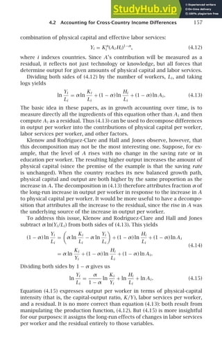
![158 Chapter 4 CROSS-COUNTRY INCOME DIFFERENCES
Data and Basic Results
Data on output and the number of workers are available from the Penn
World Tables. Hall and Jones and Klenow and Rodrı́guez-Clare estimate
physical-capital stocks using data on investment from the Penn World Tables
and reasonable assumptions about the initial stocks and depreciation. Data
on income shares suggest that α, physical capital’s share in the production
function, is around one-third for almost all countries (Gollin, 2002).
The hardest part of the analysis is to estimate the stock of labor ser-
vices, H. Hall and Jones take the simplest approach. They consider only
years of schooling. Specifically, they assume that Hi takes the form eφ(Ei )
Li ,
where Ei is the average number of years of education of workers in country
i and φ(•) is an increasing function. In the previous section, we considered
the possibility of a linear φ(•) function: φ(E) = φE. Hall and Jones argue,
however, that the microeconomic evidence suggests that the percentage in-
crease in earnings from an additional year of schooling falls as the amount
of schooling rises. On the basis of this evidence, they assume that φ(E) is a
piecewise linear function with a slope of 0.134 for E below 4 years, 0.101
for E between 4 and 8 years, and 0.068 for E above 8 years.
Armed with these data and assumptions, Hall and Jones use expression
(4.15) to estimate the contributions of physical-capital intensity, schooling,
and the residual to output per worker in each country. They summarize their
results by comparing the five richest countries in their sample with the five
poorest. Average output per worker in the rich group exceeds the average in
the poor group by a stunning factor of 31.7. On a log scale, this is a difference
of 3.5. The difference in the average [α/(1 − α)] ln(K/Y) between the two
groups is 0.6; in ln(H/L), 0.8; and in ln A, 2.1. That is, they find that only
about a sixth of the gap between the richest and poorest countries is due
to differences in physical-capital intensity, and that less than a quarter is
due to differences in schooling. Klenow and Rodrı́guez-Clare, using slightly
different assumptions, reach similar conclusions.
An additional finding from Hall and Jones’s and Klenow and Rodrı́guez-
Clare’s decompositions is that the contributions of physical capital, school-
ing, and the residual are not independent. Hall and Jones, for example, find a
substantial correlation across countries between their estimates of ln(Hi /Li )
and ln Ai (ρ = 0.52), and a modest correlation between their estimates of
[α/(1 − α)] ln(Ki /Li ) and ln Ai (ρ = 0.25); they also find a substantial corre-
lation between the two capital terms (ρ = 0.60).
More Detailed Examinations of Human Capital
Hall and Jones’s and Klenow and Rodrı́guez-Clare’s decompositions have
been extended in numerous ways. For the most part, the extensions suggest
an even larger role for the residual.](https://image.slidesharecdn.com/advanced-macroeconomics-230806183016-1212def2/85/Advanced-Macroeconomics-180-320.jpg)

![160 Chapter 4 CROSS-COUNTRY INCOME DIFFERENCES
low-income country (who has low skills) may have low wages in part not be-
cause output for a given set of inputs is low, but because he or she has few
high-skill workers to work with. And indeed, the premium to having high
skills is larger in poor countries. Hendricks finds that when he chooses an
elasticity of substitution between low-skill and high-skill workers to fit the
cross-country pattern of skill premia, he is able to explain a moderate addi-
tional part of cross-country income differences.
The combined effect of these more careful analyses of the role of human
capital is not large. For example, Hendricks finds an overall role for human-
capital differences in income differences that is slightly smaller than what
Hall and Jones estimate.
More Detailed Examinations of Physical Capital
Hall and Jones’s and Klenow and Rodríguez-Clare’s decomposition has also
been extended on the physical-capital side. The most thorough extension
is that of Hsieh and Klenow (2007). Hsieh and Klenow begin by observ-
ing that a lower capital-output ratio presumably reflects a lower average
investment-output ratio. They then note that, as a matter of accounting,
there are three possible sources of a lower investment-output ratio. First,
and most obviously, it can arise because the fraction of nominal income
devoted to investment is smaller. Second, it can arise because investment
goods are more costly (for example, because of distortionary policies or
transportation costs), so that a given amount of investment spending yields
a smaller quantity of investment (Jones, 1994). And third, it can arise be-
cause noninvestment goods have lower prices, which again has the effect
that devoting a given fraction of nominal income to investment yields a
smaller quantity of investment goods.
It has long been known that nontradable consumption goods, such as
haircuts and taxi rides, are generally cheaper in poorer countries; this is
the Balassa-Samuelson effect. The reasons for the effect are uncertain. One
possibility is that it arises because these goods use unskilled labor, which
is comparatively cheap in poor countries, more intensively. Another is that
it occurs because these goods are of lower quality in poor countries.
If lower income leads to lower prices of nontradable consumption goods,
this implies that a fall in H or A with the saving rate and the price of in-
vestment goods held fixed tends to lower the capital-output ratio. Thus, al-
though the decomposition in (4.15) (like the decomposition in [4.13]) is not
incorrect, it is probably more insightful to assign the differences in income
per worker that result from income’s impact on the price of nontradables,
and hence on investment for a given saving rate, to the underlying differ-
ences in H and A rather than to physical capital.
To see how Hsieh and Klenow decompose differences in the investment-
output ratio into the contributions of the three determinants they identify,](https://image.slidesharecdn.com/advanced-macroeconomics-230806183016-1212def2/85/Advanced-Macroeconomics-182-320.jpg)
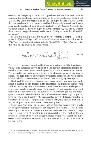


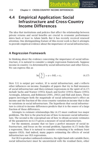

![166 Chapter 4 CROSS-COUNTRY INCOME DIFFERENCES
regression, SI −
SI . Thus regressing ln(Y/L) on
SI yields a valid estimate
of b.9
Thus, the key to addressing the second problem—how to estimate (4.17)—
is to find valid instruments. Before discussing that issue, let us return to the
first problem—how to measure social infrastructure. It is clear that any mea-
sure of social infrastructure will be imperfect. Let SI ∗
denote “true” social
infrastructure, and let
SI denote measured social infrastructure. The under-
lying relationship of interest is that between true social infrastructure and
income:
ln
Yi
Li
= a + bSI ∗
i + ei . (4.19)
True social infrastructure equals measured social infrastructure plus the
difference between true and measured social infrastructure: SI ∗
i =
SIi +
SI ∗
i −
SIi ). This allows us to rewrite (4.19) in terms of observables and other
factors:
ln
Yi
Li
= a + b
SIi + b(SI ∗
i −
SIi ) + ei
(4.20)
≡ a + b
SIi + vi .
To consider what happens if we estimate (4.20) by OLS, consider the case
of classical measurement error:
SIi = SI ∗
i +wi , where w is uncorrelated with
SI ∗
. In this case, the right-hand-side variable in the regression is SI ∗
+w, and
one component of the composite residual, v, is −bw. Thus if b is positive,
the measurement error causes negative correlation between the right-hand-
side variable and the residual. Thus again there is omitted-variable bias, but
now it biases the estimate of b down rather than up.
Since measurement error leads to omitted-variable bias, the solution is
again instrumental variables. That is, to obtain valid estimates of the im-
pact of social infrastructure on income, we need to find variables that are
not systematically correlated both with the measurement error in social in-
frastructure (the b(SI ∗
−
SI ) component of the composite residual in [4.20],
v) and with forces other than social infrastructure that affect income (the e
component).
9
The fact that
SI is based on estimated coefficients causes two complications. First, the
uncertainty about the estimated coefficients must be accounted for in finding the standard
error in the estimate of b; this is done in the usual formulas for the standard errors of
instrumental-variables estimates. Second, the fact that the first-stage coefficients are esti-
mated introduces some correlation between
SI and e in the same direction as the correlation
between SI and e. This correlation disappears as the sample size becomes large; thus IV is
consistent but not unbiased. If the instruments are only moderately correlated with the
right-hand-side variable, however, the bias in finite samples can be large. See, for example,
Staiger and Stock (1997).](https://image.slidesharecdn.com/advanced-macroeconomics-230806183016-1212def2/85/Advanced-Macroeconomics-188-320.jpg)


![174 Chapter 4 CROSS-COUNTRY INCOME DIFFERENCES
affect capital accumulation, such as cultural attitudes toward thrift and
education, are important as well.
Although externalities from capital attracted considerable attention in
early work on new growth theory, several types of evidence suggest that they
are not crucial to cross-country income differences. First, the hypothesis of
large positive externalities from physical capital predicts that an increase
in the saving rate raises income by even more than conventional growth-
accounting calculations imply. Thus the absence of a noticeable correlation
between the saving rate and income is consistent with this view only if there
are negative influences on income that are correlated with the saving rate.
Second, there is no compelling microeconomic evidence of local external-
ities from capital large enough to account for the enormous income differ-
ences we observe. Third, highly statist economies have often been very suc-
cessful at the accumulation of physical and human capital, and at achieving
higher capital-output ratios than their market-oriented counterparts. But
these countries’ economic performance has been generally dismal.
Finally, Bils and Klenow (2000) observe that we can use the simple fact
that there is not technological regress to place an upper bound on the exter-
nalities from human capital. In the United States and other industrialized
countries, the average education of the labor force has been rising at an
average rate of about 0.1 years each year. An additional year of education
typically raises an individual’s earnings by about 10 percent. If the social
return to education were double this, increases in education would be rais-
ing average output per worker by about 2 percent per year (see equation
[4.15], for example). But this would account for essentially all growth of
output per worker. Since technology cannot be regressing, we can conclude
that the social return to education cannot be greater than this. And if we
are confident that technology is improving, we can conclude that the social
return to education is less than this.
For these reasons, recent work on cross-country income differences for
the most part does not emphasize externalities from capital.15
Empirical Application: Geography, Colonialism, and
Economic Development
A striking fact about cross-country income differences is that average in-
comes are much lower closer to the equator. Figure 4.1, from Bloom and
Sachs (1998), shows this pattern dramatically. Average incomes in countries
15
Early theoretical models of externalities from capital include P. Romer (1986), Lucas
(1988), and Rebelo (1991). When applied naively to the issue of cross-country income differ-
ences, these models tend to have the counterfactual implication that countries with higher
saving rates have permanently higher growth rates. Later models of capital externalities
that focus explicitly on the issue of income differences among countries generally avoid
this implication. See, for example, Basu and Weil (1999).](https://image.slidesharecdn.com/advanced-macroeconomics-230806183016-1212def2/85/Advanced-Macroeconomics-196-320.jpg)


![4.6 Differences in Growth Rates 179
Convergence to Balanced Growth Paths
We begin with the case where the underlying determinants of long-run rela-
tive income per person across countries are constant over time. That is, we
begin by ignoring changes in relative saving rates, years of education, and
long-run determinants of output for a given set of inputs.
Countries’ incomes do not jump immediately to their long-run paths. For
example, if part of a country’s capital stock is destroyed in a war, capital
returns to its long-run path only gradually. During the return, capital per
worker is growing more rapidly than normal, and so output per worker is
growing more rapidly than normal. More generally, one source of differ-
ences in growth rates across countries is differences in the countries’ initial
positions relative to their long-run paths. Countries that begin below their
long-run paths grow more rapidly than countries that begin above.
To see this more formally, assume for simplicity that differences in out-
put per worker across countries stem only from differences in physical cap-
ital per worker. That is, human capital per worker and output for given in-
puts are the same in all countries. Assume that output is determined by a
standard production function, Yi (t) = F (Ki (t),A(t)Li (t)), with constant re-
turns. Because of the constant-returns assumption, we can write output per
worker in country i as
Yi (t)
Li (t)
= A(t)f (ki (t)). (4.21)
(As in our earlier models, k ≡ K/(AL) and f (k) ≡ F (k,1).) By assumption, the
path of A is the same in all countries. Thus (4.21) implies that differences
in growth come only from differences in the behavior of k.
In the Solow and Ramsey models, each economy has a balanced-growth-
path value of k, and the rate of change of k is approximately proportional
to its departure from its balanced-growth-path value (see Sections 1.5 and
2.6). If we assume that the same is true here, we have
˙
ki (t) = λ[k∗
i − ki (t)], (4.22)
where k∗
i is the balanced-growth-path value of k in country i and λ 0 is the
rate of convergence. Equation (4.22) implies that when a country is farther
below its balanced growth path, its capital per unit of effective labor rises
more rapidly, and so its growth in income per worker is greater.
There are two possibilities concerning the values of k∗
i . The first is that
they are the same in all countries. In this case, all countries have the same
income per worker on their balanced growth paths. Differences in average
income stem only from differences in where countries stand relative to the
common balanced growth path. Thus in this case, the model predicts that
the lower a country’s income per person, the faster its growth. This is known
as unconditional convergence.](https://image.slidesharecdn.com/advanced-macroeconomics-230806183016-1212def2/85/Advanced-Macroeconomics-201-320.jpg)

![4.6 Differences in Growth Rates 181
that economies have balanced growth paths they would converge to in the
absence of shocks. Recall equation (4.22): ˙
ki (t) = λ[k∗
i − ki (t)]. We want to
consider growth over some interval of time where k∗
i need not be constant.
To see the issues involved, it is easiest to assume that time is discrete and to
consider growth over just two periods. Assume that the change in ki from
period t to period t + 1, denoted, kit+1, depends on the period-t values of
k∗
i and ki . The equation analogous to (4.22) is thus
kit +1 = λ(k∗
it − kit), (4.23)
with λ assumed to be between 0 and 1. The change in ki from t to t + 2 is
therefore
kit +1 + kit +2 = λ(k∗
it − kit) + λ(k∗
it +1 − kit +1). (4.24)
To interpret this expression, rewrite k∗
it +1 as k∗
it + k∗
it +1 and kit +1 as
kit + kit +1. Thus (4.24) becomes
kit +1 + kit +2 = λ(k∗
it − kit) + λ(k∗
it + k∗
it +1 − kit − kit +1)
= λ(k∗
it − kit) + λ[k∗
it + k∗
it +1 − kit − λ(k∗
it − kit)]
= [λ+ λ(1 − λ)](k∗
it − kit) + λk∗
it +1,
(4.25)
where the second line uses (4.23) to substitute for kit +1.
It is also useful to consider the continuous-time case. One can show that
if k∗
i does not change discretely, then (4.22) implies that the change in k
over some interval, say from 0 to T, is
ki (T ) − ki (0) = (1 − e−λT
)[k∗
i (0) − ki (0)]
(4.26)
+
T
τ=0
(1 − e−λ(T−τ)
)˙
k∗
i (τ) dτ.
Expressions (4.25) and (4.26) show that we can decompose that change
in k over an interval into two terms. The first depends on the country’s
initial position relative to its balanced growth path. This is the conditional-
convergence effect we discussed above. The second term depends on
changes in the balanced growth path during the interval. A rise in the
balanced-growth-path value of k, for example, raises growth. Further, as the
expression for the continuous-time case shows (and as one would expect),
such a rise has a larger effect if it occurs earlier in the interval.
For simplicity, we have focused on physical capital. But analogous results
apply to human capital and efficiency: growth depends on countries’ start-
ing points relative to their balanced growth paths and on changes in their
balanced growth paths.
This analysis shows that the issue of convergence is more complicated
than our earlier discussion suggests. Overall convergence depends not only
on the distribution of countries’ initial positions relative to their long-run](https://image.slidesharecdn.com/advanced-macroeconomics-230806183016-1212def2/85/Advanced-Macroeconomics-203-320.jpg)


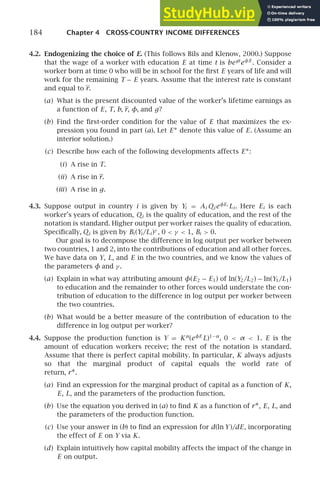
![Problems 185
4.5. (This follows Mankiw, D. Romer, and Weil, 1992.) Suppose output is given by
Y(t) = K(t)α
H(t)β
[A(t)L(t)]1−α−β
, α 0, β 0, α + β 1. Here L is the number
of workers and H is their total amount of skills. The remainder of the notation
is standard. The dynamics of the inputs are L̇(t) = nL(t), Ȧ(t) = gA(t), K̇(t) =
skY(t) − δK(t), Ḣ (t) = shY(t) − δH(t), where 0 sk 1, 0 sh 1, and n + g + δ
0. L(0), A(0), K(0), and H(0) are given, and are all strictly positive. Finally, define
y(t) ≡ Y(t)/[A(t)L(t)], k(t) ≡ K(t)/[A(t)L(t)], and h(t) ≡ H(t)/[A(t)L(t)].
(a) Derive an expression for y(t) in terms of k(t) and h(t) and the parameters
of the model.
(b) Derive an expression for k̇(t) in terms of k(t) and h(t) and the parameters
of the model. In (k,h) space, sketch the set of points where k̇ = 0.
(c) Derive an expression for ḣ (t) in terms of k(t) and h(t) and the parameters
of the model. In (k,h) space, sketch the set of points where ḣ = 0.
(d) Does the economy converge to a balanced growth path? Why or why not?
If so, what is the growth rate of output per worker on the balanced growth
path? If not, in general terms what is the behavior of output per worker
over time?
4.6. Consider the model in Problem 4.5.
(a) What are the balanced-growth-path values of k and h in terms of sk, sh, and
the other parameters of the model?
(b) Suppose α = 1/3 and β = 1/2. Consider two countries, A and B, and
suppose that both sk and sh are twice as large in Country A as in Country B
and that the countries are otherwise identical. What is the ratio of the
balanced-growth-path value of income per worker in Country A to its value
in Country B implied by the model?
(c) Consider the same assumptions as in part (b). What is the ratio of the
balanced-growth-path value of skills per worker in Country A to its value
in Country B implied by the model?
4.7. (This follows Jones, 2002a.) Consider the model of Section 4.1 with the as-
sumption that G(E) = eφE
. Suppose, however, that E, rather than being con-
stant, is increasing steadily: Ė(t) = m, where m 0. Assume that, despite the
steady increase in the amount of education people are getting, the growth
rate of the number of workers is constant and equal to n, as in the basic
model.
(a) With this change in the model, what is the long-run growth rate of output
per worker?
(b) In the United States over the past century, if we measure E as years of
schooling, φ ≈ 0.1 and m ≈ 1/15. Overall growth of output per worker
has been about 2 percent per year. In light of your answer to (a), approx-
imately what fraction of this overall growth has been due to increasing
education?
(c) Can Ė(t) continue to equal m 0 forever? Explain.](https://image.slidesharecdn.com/advanced-macroeconomics-230806183016-1212def2/85/Advanced-Macroeconomics-207-320.jpg)
![186 Chapter 4 CROSS-COUNTRY INCOME DIFFERENCES
4.8. Consider the following model with physical and human capital:
Y (t) = [(1 − aK )K(t)]α
[(1 − aH)H(t)]1−α
, 0 α 1, 0 aK 1, 0 aH 1,
K̇(t) = sY (t) − δK K(t),
Ḣ (t) = B[aK K(t)]γ
[aH H(t)]φ
[A(t)L(t)]1−γ −φ
− δH H(t), γ 0, φ 0, γ + φ 1,
L̇(t) = nL(t),
Ȧ(t) = gA(t),
where aK and aH are the fractions of the stocks of physical and human capital
used in the education sector.
This model assumes that human capital is produced in its own sector
with its own production function. Bodies (L) are useful only as something to
be educated, not as an input into the production of final goods. Similarly,
knowledge (A) is useful only as something that can be conveyed to students,
not as a direct input to goods production.
(a) Define k = K/(AL) and h = H/(AL). Derive equations for k̇ and ḣ.
(b) Find an equation describing the set of combinations of h and k such that
k̇ = 0. Sketch in (h,k) space. Do the same for ḣ = 0.
(c) Does this economy have a balanced growth path? If so, is it unique? Is
it stable? What are the growth rates of output per person, physical cap-
ital per person, and human capital per person on the balanced growth
path?
(d) Suppose the economy is initially on a balanced growth path, and that
there is a permanent increase in s. How does this change affect the path
of output per person over time?
4.9. Increasing returns in a model with human capital. (This follows Lucas, 1988.)
Suppose that Y (t) = K(t)α
[(1 − aH)H(t)]β
, Ḣ (t) = BaH H(t), and K̇(t) = sY (t).
Assume 0 α 1, 0 β 1, and α + β 1.20
(a) What is the growth rate of H ?
(b) Does the economy converge to a balanced growth path? If so, what are
the growth rates of K and Y on the balanced growth path?
4.10. (A different form of measurement error.) Suppose the true relationship be-
tween social infrastructure (SI ) and log income per person (y) is yi = a +
bSIi + ei . There are two components of social infrastructure, SI A
and SI B
(with SIi = SI A
i + SI B
i ), and we only have data on one of the components, SI A
.
Both SI A
and SI B
are uncorrelated with e. We are considering running an OLS
regression of y on a constant and SI A
.
(a) Derive an expression of the form, yi = a + bSI A
i + other terms.
20
Lucas’s model differs from this formulation by letting aH and s be endogenous and
potentially time-varying, and by assuming that the social and private returns to human
capital differ.](https://image.slidesharecdn.com/advanced-macroeconomics-230806183016-1212def2/85/Advanced-Macroeconomics-208-320.jpg)
![Problems 187
(b) Use your answer to part (a) to determine whether an OLS regression of y
on a constant and SI A
will produce an unbiased estimate of the impact
of social infrastructure on income if:
(i) SI A
and SI B
are uncorrelated.
(ii) SI A
and SI B
are positively correlated.
4.11. Briefly explain whether each of the following statements concerning a cross-
country regression of income per person on a measure of social infrastructure
is true or false:
(a) “If the regression is estimated by ordinary least squares, it shows the
effect of social infrastructure on output per person.”
(b) “If the regression is estimated by instrumental variables using variables
that are not affected by social infrastructure as instruments, it shows the
effect of social infrastructure on output per person.”
(c) “If the regression is estimated by ordinary least squares and has a high
R2
, this means that there are no important influences on output per per-
son that are omitted from the regression; thus in this case, the coefficient
estimate from the regression is likely to be close to the true effect of social
infrastructure on output per person.”
4.12. Convergence regressions.
(a) Convergence. Let yi denote log output per worker in country i. Suppose
all countries have the same balanced-growth-path level of log income
per worker, y∗. Suppose also that yi evolves according to dyi (t)/dt =
−λ[yi (t) − y∗].
(i) What is yi (t) as a function of yi (0), y∗, λ, and t?
(ii) Suppose that yi (t) in fact equals the expression you derived in
part (i) plus a mean-zero random disturbance that is uncorrelated
with yi (0). Consider a cross-country growth regression of the form
yi (t) − yi (0) = α + βyi (0) + εi . What is the relation between β, the co-
efficient on yi (0) in the regression, and λ, the speed of convergence?
(Hint: For a univariate OLS regression, the coefficient on the right-
hand-side variable equals the covariance between the right-hand-side
and left-hand-side variables divided by the variance of the right-hand-
side variable.) Given this, how could you estimate λ from an estimate
of β?
(iii) If β in part (ii) is negative (so that rich countries on average grow less
than poor countries), is Var(yi (t)) necessarily less than Var(yi (0)), so
that the cross-country variance of income is falling? Explain. If β is
positive, is Var(yi (t)) necessarily more than Var(yi (0))? Explain.
(b) Conditional convergence. Suppose y∗
i = a + bXi , and that dyi (t)/dt =
−λ[yi (t) − y∗
i ].
(i) What is yi (t) as a function of yi (0), Xi , λ, and t?
(ii) Suppose that yi (0) = y∗
i +ui and that yi (t) equals the expression you
derived in part (i) plus a mean-zero random disturbance, ei , where](https://image.slidesharecdn.com/advanced-macroeconomics-230806183016-1212def2/85/Advanced-Macroeconomics-209-320.jpg)


![196 Chapter 5 REAL-BUSINESS-CYCLE THEORY
Output is divided among consumption (C), investment (I ), and govern-
ment purchases (G). Fraction δ of capital depreciates each period. Thus the
capital stock in period t + 1 is
Kt +1 = Kt + It − δKt
= Kt + Yt − Ct − Gt − δKt .
(5.2)
The government’s purchases are financed by lump-sum taxes that are as-
sumed to equal the purchases each period.8
Labor and capital are paid their marginal products. Thus the real wage
and the real interest rate in period t are
wt = (1 − α)Kα
t (At Lt )−α
At
= (1 − α)
Kt
At Lt
α
At ,
(5.3)
rt = α
At Lt
Kt
1−α
− δ. (5.4)
The representative household maximizes the expected value of
U =
∞
t = 0
e−ρt
u(ct,1 − ℓt)
Nt
H
. (5.5)
u(•) is the instantaneous utility function of the representative member of the
household, and ρ is the discount rate.9
Nt is population and H is the number
of households; thus Nt/H is the number of members of the household.
Population grows exogenously at rate n:
ln Nt = N + nt, n ρ. (5.6)
Thus the level of Nt is given by Nt = eN+nt
.
The instantaneous utility function, u(•), has two arguments. The first is
consumption per member of the household, c. The second is leisure per
member, which is the difference between the time endowment per member
(normalized to 1 for simplicity) and the amount each member works, ℓ.
8
As in the Ramsey model, the choice between debt and tax finance in fact has no impact
on outcomes in this model. Thus the assumption of tax finance is made just for expositional
convenience. Section 12.2 describes why the form of finance is irrelevant in models like
this one.
9
The usual way to express discounting in a discrete-time model is as 1/(1 + ρ)t
rather
than as e−ρt
. But because of the log-linear structure of this model, the exponential formu-
lation is more natural here. There is no important difference between the two approaches,
however. Specifically, if we define ρ′
= eρ
−1, then e−ρt
= 1/(1+ρ′
)t
. The log-linear structure
of the model is also the reason behind the exponential formulations for population growth
and for trend growth of technology and government purchases (see equations [5.6], [5.8],
and [5.10]).](https://image.slidesharecdn.com/advanced-macroeconomics-230806183016-1212def2/85/Advanced-Macroeconomics-218-320.jpg)
![198 Chapter 5 REAL-BUSINESS-CYCLE THEORY
In this case, the household’s objective function is just ln c + b ln(1 − ℓ), and
its budget constraint is c = wℓ.
The Lagrangian for the household’s maximization problem is
L = ln c + b ln(1 − ℓ) + λ(wℓ − c). (5.12)
The first-order conditions for c and ℓ, respectively, are
1
c
− λ = 0, (5.13)
−
b
1 − ℓ
+ λw = 0. (5.14)
Since the budget constraint requires c = wℓ, (5.13) implies λ = 1/(wℓ).
Substituting this into (5.14) yields
−
b
1 − ℓ
+
1
ℓ
= 0. (5.15)
The wage does not enter (5.15). Thus labor supply (the value of ℓ that sat-
isfies [5.15]) is independent of the wage. Intuitively, because utility is loga-
rithmic in consumption and the household has no initial wealth, the income
and substitution effects of a change in the wage offset each other.
The fact that the level of the wage does not affect labor supply in the
static case does not mean that variations in the wage do not affect labor
supply when the household’s horizon is more than one period. This can
be seen most easily when the household lives for two periods. Continue to
assume that it has no initial wealth and that it has only one member; in
addition, assume that there is no uncertainty about the interest rate or the
second-period wage.
The household’s lifetime budget constraint is now
c1 +
1
1 + r
c2 = w1ℓ1 +
1
1 + r
w2ℓ2, (5.16)
where r is the real interest rate. The Lagrangian is
L = ln c1 + b ln(1 − ℓ1) + e−ρ
[ln c2 + b ln(1 − ℓ2)]
+ λ
w1ℓ1 +
1
1 + r
w2ℓ2 − c1 −
1
1 + r
c2
.
(5.17)
The household’s choice variables are c1, c2, ℓ1, and ℓ2. Only the first-
order conditions for ℓ1 and ℓ2 are needed, however, to show the effect of the
relative wage in the two periods on relative labor supply. These conditions
are
b
1 − ℓ1
= λw1, (5.18)
e−ρ
b
1 − ℓ2
=
1
1 + r
λw2. (5.19)](https://image.slidesharecdn.com/advanced-macroeconomics-230806183016-1212def2/85/Advanced-Macroeconomics-220-320.jpg)
![200 Chapter 5 REAL-BUSINESS-CYCLE THEORY
equation using the informal approach we used in equations (2.22)–(2.23) to
derive the Euler equation.10
Consider the household in period t. Suppose it reduces current consump-
tion per member by a small amount c and then uses the resulting greater
wealth to increase consumption per member in the next period above what
it otherwise would have been. If the household is behaving optimally, a
marginal change of this type must leave expected utility unchanged.
Equations (5.5) and (5.7) imply that the marginal utility of consumption
per member in period t, ct, is e−ρt
(Nt/H )(1/ct ). Thus the utility cost of this
change is e−ρt
(Nt/H )(c/ct ). Since the household has en
times as many
members in period t + 1 as in period t, the increase in consumption per
member in period t + 1, ct + 1, is e−n
(1 + rt + 1) c. The marginal utility of
period-t+1 consumption per member is e−ρ(t + 1)
(Nt + 1/H )(1/ct + 1). Thus
the expected utility benefit as of period t is Et [e−ρ(t + 1)
(Nt + 1/H )e−n
(1 +
rt + 1)/ct +1] c, where Et denotes expectations conditional on what the house-
hold knows in period t (that is, conditional on the history of the economy
up through period t ). Equating the costs and expected benefits implies
e−ρt Nt
H
c
ct
= Et
e−ρ(t + 1) Nt +1
H
e−n 1
ct +1
(1 + rt +1)
c. (5.22)
Since e−ρ(t +1)
(Nt +1/H )e−n
is not uncertain and since Nt +1 = Nt en
, this con-
dition simplifies to
1
ct
= e−ρ
Et
1
ct +1
(1 + rt +1)
. (5.23)
This is the analogue of equation (2.20) in the Ramsey model.
Note that the expression on the right-hand side of (5.23) is not the same
as e−ρ
Et [1/ct +1]Et [1 + rt +1]. That is, the tradeoff between present and fu-
ture consumption depends not just on the expectations of future marginal
utility and of the rate of return, but also on their interaction. Specifically,
the expectation of the product of two variables equals the product of their
expectations plus their covariance. Thus (5.23) implies
1
ct
= e−ρ
Et
1
ct +1
Et [1 + rt +1] + Cov
1
ct +1
,1 + rt +1
, (5.24)
where Cov(1/ct +1,1 + rt +1) denotes the covariance of 1/ct +1 and 1 + rt +1.
Suppose, for example, that when rt +1 is high, ct +1 is also high. In this case,
Cov(1/ct +1,1 + rt +1) is negative; that is, the return to saving is high in the
times when the marginal utility of consumption is low. This makes saving
less attractive than it is if 1/ct +1 and rt +1 are uncorrelated, and thus tends
to raise current consumption.
Chapter 8 discusses the impact of uncertainty on optimal consumption
further.
10
The household’s problem can be analyzed more formally using dynamic programming
(see Section 10.4 or Ljungqvist and Sargent, 2004). This also yields (5.23) below.](https://image.slidesharecdn.com/advanced-macroeconomics-230806183016-1212def2/85/Advanced-Macroeconomics-222-320.jpg)
![5.5 A Special Case of the Model 201
The Tradeoff between Consumption and Labor Supply
The household chooses not only consumption at each date, but also labor
supply. Thus a second first-order condition for the household’s optimiza-
tion problem relates its current consumption and labor supply. Specifically,
imagine the household increasing its labor supply per member in period t
by a small amount ℓ and using the resulting income to increase its con-
sumption in that period. Again if the household is behaving optimally, a
marginal change of this type must leave expected utility unchanged.
From equations (5.5) and (5.7), the marginal disutility of labor supply
in period t is e−ρt
(Nt /H )[b/(1 − ℓt)]. Thus the change has a utility cost of
e−ρt
(Nt /H )[b/(1 − ℓt)] ℓ. And since the change raises consumption per
member by wt ℓ, it has a utility benefit of e−ρt
(Nt /H )(1/ct)wt ℓ. Equating
the cost and benefit gives us
e−ρt Nt
H
b
1 − ℓt
ℓ = e−ρt Nt
H
1
ct
wt ℓ, (5.25)
or
ct
1 − ℓt
=
wt
b
. (5.26)
Equation (5.26) relates current leisure and consumption, given the wage. Be-
cause it involves current variables, which are known, uncertainty does not
enter. Equations (5.23) and (5.26) are the key equations describing house-
holds’ behavior.
5.5 A Special Case of the Model
Simplifying Assumptions
The model of Section 5.3 cannot be solved analytically. The basic problem
is that it contains a mixture of ingredients that are linear—such as depre-
ciation and the division of output into consumption, investment, and gov-
ernment purchases—and ones that are log-linear—such as the production
function and preferences. In this section, we therefore investigate a simpli-
fied version of the model.
Specifically, we make two changes to the model: we eliminate govern-
ment, and we assume 100 percent depreciation each period.11
Thus
11
With these changes, the model corresponds to a one-sector version of Long and
Plosser’s (1983) real-business-cycle model. McCallum (1989) investigates this model. In addi-
tion, except for the assumption of δ = 1, the model corresponds to the basic case considered
by Prescott (1986). It is straightforward to assume that a constant fraction of output is pur-
chased by the government instead of eliminating government altogether.](https://image.slidesharecdn.com/advanced-macroeconomics-230806183016-1212def2/85/Advanced-Macroeconomics-223-320.jpg)

![5.5 A Special Case of the Model 203
capital to have offsetting income and substitution effects on saving. It is
the fact that s is constant that allows the model to be solved analytically.
Consider (5.23) first; this condition is 1/ct = e−ρ
Et [(1 + rt +1)/ct +1]. Since
ct = (1 − st )Yt/Nt, rewriting (5.23) along the lines just suggested gives us
− ln
(1 − st )
Yt
Nt
= −ρ + ln Et
1 + rt +1
(1 − st +1)Yt +1/Nt +1
. (5.29)
Equation (5.28) implies that 1 + rt +1 equals α(A t +1 L t +1/Kt +1)1−α
, or αYt +1/
Kt +1. In addition, the assumption of 100 percent depreciation implies that
Kt +1 = Yt − Ct = stYt. Substituting these facts into (5.29) yields
− ln(1 − st ) − ln Yt + ln Nt
= −ρ + ln Et
αYt +1
Kt +1(1 − st +1)Yt +1/Nt +1
= −ρ + ln Et
αNt +1
st (1 − st +1)Yt
= −ρ + ln α + ln Nt + n − ln st − ln Yt + ln Et
1
1 − st +1
,
(5.30)
where the final line uses the facts that α, Nt +1, st, and Yt are known at date t
and that N is growing at rate n. Equation (5.30) simplifies to
ln st − ln(1 − st) = −ρ + n + ln α + ln Et
1
1 − st +1
. (5.31)
Crucially, the two state variables, A and K, do not enter (5.31). This im-
plies that there is a constant value of s that satisfies this condition. To see
this, note that if s is constant at some value ŝ, then st +1 is not uncertain,
and so Et [1/(1 − st +1)] is simply 1/(1 − ŝ). Thus (5.31) becomes
ln ŝ = ln α + n − ρ, (5.32)
or
ŝ = αen−ρ
. (5.33)
Thus the model has a solution where the saving rate is constant.
Now consider (5.26), which states ct /(1 − ℓt ) = wt /b. Since ct = Ct /Nt =
(1 − ŝ)Yt /Nt, we can rewrite this condition as
ln
(1 − ŝ)
Yt
Nt
− ln(1 − ℓt ) = ln wt − ln b. (5.34)](https://image.slidesharecdn.com/advanced-macroeconomics-230806183016-1212def2/85/Advanced-Macroeconomics-225-320.jpg)
![5.5 A Special Case of the Model 205
stock.13
In particular, the production function, Yt = Kα
t (At Lt )1−α
, implies
ln Yt = αln Kt + (1 − α)(ln At + ln Lt ). (5.38)
We know that Kt = ŝYt −1 and Lt = ℓ̂Nt; thus
ln Yt = αln ŝ + αln Yt −1 + (1 − α)(ln At + ln ℓ̂ + ln Nt )
= αln ŝ + αln Yt −1 + (1 − α)(A + gt)
+ (1 − α)Ãt + (1 − α)(ln ℓ̂ + N + nt),
(5.39)
where the last line uses the facts that ln At = A + gt + Ãt and ln Nt = N + nt
(see [5.6] and [5.8]).
The two components of the right-hand side of (5.39) that do not follow
deterministic paths are αln Yt −1 and (1−α)Ãt. It must therefore be possible
to rewrite (5.39) in the form
Ỹt = αỸt −1 + (1 − α)Ãt, (5.40)
where Ỹt is the difference between ln Yt and the value it would take if ln At
equaled A + gt each period (see Problem 5.14 for the details).
To see what (5.40) implies concerning the dynamics of output, note that
since it holds each period, it implies Ỹt −1 = αỸt−2 + (1 − α)Ãt −1, or
Ãt −1 =
1
1 − α
Ỹt −1 − αỸt −2 . (5.41)
Recall that (5.9) states that Ãt = ρA Ãt −1 + εA,t. Substituting this fact and
(5.41) into (5.40), we obtain
Ỹt = αỸt −1 + (1 − α)(ρA Ãt −1 + εA,t )
= αỸt −1 + ρA (Ỹt −1 − αỸt−2 ) + (1 − α)εA,t
= (α + ρA )Ỹt −1 − αρA Ỹt−2 + (1 − α)εA,t.
(5.42)
Thus, departures of log output from its normal path follow a second-order
autoregressive process; that is, Ỹ can be written as a linear combination of
its two previous values plus a white-noise disturbance.14
The combination of a positive coefficient on the first lag of Ỹt and a nega-
tive coefficient on the second lag can cause output to have a “hump-shaped”
13
The discussion that follows is based on McCallum (1989).
14
Readers who are familiar with the use of lag operators can derive (5.42) using that
approach. In lag operator notation, Ỹt −1 is LỸ t, where L maps variables to their previ-
ous period’s value. Thus (5.40) can be written as Ỹ t = αLỸ t + (1 − α)Ãt, or (1 − αL )Ỹ t =
(1 − α)Ãt. Similarly, we can rewrite (5.9) as (1 − ρA L )Ãt = εA,t, or Ãt = (1 − ρA L )−1
εA,t.
Thus we have (1 − αL )Ỹ t = (1 − α)(1 − ρA L )−1
εA,t. “Multiplying” through by 1 − ρA L yields
(1 − αL )(1 − ρA L )Ỹ t = (1 − α)εA,t, or [1 − (α + ρA )L + αρA L2
]Ỹ t = (1 − α)εA,t. This is equi-
valent to Ỹ t = (α + ρA )LỸ t − αρA L2
Ỹ t + (1 − α)εA,t, which corresponds to (5.42). (See Sec-
tion 7.3 for a discussion of lag operators and of the legitimacy of manipulating them in these
ways.)](https://image.slidesharecdn.com/advanced-macroeconomics-230806183016-1212def2/85/Advanced-Macroeconomics-227-320.jpg)

![208 Chapter 5 REAL-BUSINESS-CYCLE THEORY
log consumption and log employment are linear functions of the logs of
K, A, and G, and that consumption and employment are equal to their
balanced-growth-path values when K, A, and G are all equal to theirs. Since
we are building a version of the model that is log-linear around the balanced
growth path by construction, we know that these conditions must hold. To
solve the model, we must determine the values of the a’s.
As with the simple version of the model, we will focus on the two condi-
tions for household optimization, (5.23) and (5.26). For a set of a’s to be a
solution to the model, they must imply that households are satisfying these
conditions. It turns out that the restrictions that this requirement puts on
the a’s fully determine them, and thus tell us the solution to the model.
This solution method is known as the method of undetermined coeffi-
cients. The idea is to use theory (or, in some cases, educated guesswork)
to find the general functional form of the solution, and then to determine
what values the coefficients in the functional form must take to satisfy the
equations of the model. This method is useful in many situations.
The Intratemporal First-Order Condition
Begin by considering households’ first-order condition for the tradeoff be-
tween current consumption and labor supply, ct /(1 − ℓt ) = wt /b (equa-
tion [5.26]). Using equation (5.3), wt = (1 − α)[Kt/(At Lt )]α
At, to substitute
for the wage and taking logs, we can write this condition as
ln ct − ln(1 − ℓt ) = ln
1 − α
b
+ (1 − α) ln At + αln Kt − αln Lt. (5.45)
We want to find a first-order Taylor-series approximation to this expres-
sion in the logs of the variables of the model around the balanced growth
path the economy would follow if there were no shocks. Approximating the
right-hand side is straightforward: the difference between the actual value
of the right-hand side and its balanced-growth-path value is (1 − α)Ãt +
αK̃t − αL̃t. To approximate the left-hand side, note first that since popu-
lation growth is not affected by the shocks, the log of consumption per
worker differs from its balanced-growth-path value only to the extent that
the log of total consumption differs from its balanced-growth-path value.
Thus c̃t = C̃t. Similarly, ℓ̃t = L̃t. The derivative of the left-hand side of (5.45)
with respect to ln ct is simply 1. The derivative with respect to ln ℓt at ℓt = ℓ∗
is ℓ∗/(1−ℓ∗), where ℓ∗ is the value of ℓ on the balanced growth path. Thus,
log-linearizing (5.45) around the balanced growth path yields
C̃t +
ℓ∗
1 − ℓ∗ L̃t = (1 − α)Ãt + αK̃t − αL̃t. (5.46)](https://image.slidesharecdn.com/advanced-macroeconomics-230806183016-1212def2/85/Advanced-Macroeconomics-230-320.jpg)
![5.6 Solving the Model in the General Case 209
We can now use the fact that C̃t and L̃t are linear functions of K̃t, Ãt, and
G̃t. Substituting (5.43) and (5.44) into (5.46) yields
aCK K̃t + aCAÃt + aCGG̃t +
ℓ∗
1 − ℓ∗ + α
(aLK K̃t + aLAÃt + aLGG̃t)
(5.47)
= αK̃t + (1 − α)Ãt .
Equation (5.47) must hold for all values of K̃, Ã, and G̃. If it does not, then
for some combinations of K̃, Ã, and G̃, households are not satisfying their
intratemporal first-order condition. Thus the coefficients on K̃ on the two
sides of (5.47) must be equal, and similarly for the coefficients on à and on
G̃. The a’s must therefore satisfy
aCK +
ℓ∗
1 − ℓ∗ + α
aLK = α, (5.48)
aCA +
ℓ∗
1 − ℓ∗ + α
aLA = 1 − α, (5.49)
aCG +
ℓ∗
1 − ℓ∗ + α
aLG = 0. (5.50)
To understand these conditions, consider first (5.50), which relates the
responses of consumption and employment to movements in government
purchases. Government purchases do not directly enter (5.45); that is, they
do not affect the wage for a given level of labor supply. If households in-
crease their labor supply in response to an increase in government pur-
chases, the wage falls and the marginal disutility of working rises. Thus,
they will do this only if the marginal utility of consumption is higher—
that is, if consumption is lower. Thus if labor supply and consumption
respond to changes in government purchases, they must move in oppo-
site directions. Equation (5.50) tells us not only this qualitative result, but
also how the movements in labor supply and consumption must be
related.
Now consider an increase in A (equation [5.49]). An improvement in tech-
nology raises the wage for a given level of labor supply. Thus if neither la-
bor supply nor consumption responds, households can raise their utility by
working more and increasing their current consumption. Households must
therefore increase either labor supply or consumption (or both); this is what
is captured in (5.49).
Finally, the restrictions that (5.45) puts on the responses of labor supply
and consumption to movements in capital are similar to the restrictions it
puts on their responses to movements in technology. The only difference
is that the elasticity of the wage with respect to capital, given L, is α rather
than 1 − α. This is what is shown in (5.48).](https://image.slidesharecdn.com/advanced-macroeconomics-230806183016-1212def2/85/Advanced-Macroeconomics-231-320.jpg)
![210 Chapter 5 REAL-BUSINESS-CYCLE THEORY
The Intertemporal First-Order Condition
The analysis of the first-order condition relating current consumption and
next period’s consumption, 1/ct = e−ρ
Et [(1 + rt +1)/ct +1] (equation [5.23]), is
more complicated. The basic idea is the following. Begin by defining Z̃t +1 as
the difference between the log of (1 + rt +1)/ct +1 and the log of its balanced-
growth-path value. Then use equation (5.4) for rt +1 to express 1 + rt +1 in
terms of Kt +1, At +1, and Lt +1. This allows us to approximate Z̃t +1 in terms
of K̃t +1, Ãt +1, L̃t +1 and C̃t +1. Now note that since (5.43) and (5.44) hold at
each date, they imply
C̃t +1 ≃ aCK K̃t +1 + aCAÃt +1 + aCGG̃t +1, (5.51)
L̃t +1 = aLK K̃t +1 + aLAÃt +1 + aLGG̃t +1. (5.52)
These equations allow us to express Z̃t +1 in terms of K̃t +1, Ãt +1, and G̃t +1.
Since K̃t +1 is an endogenous variable, we need to eliminate it from the
expression for Z̃t +1. Specifically, we can log-linearize the equation of motion
for capital, (5.2), to write K̃t +1 in terms of K̃t, Ãt, G̃t, L̃t, and C̃t, and then
use (5.43) and (5.44) to substitute for L̃t and C̃t. This yields an equation of
the form
K̃t +1 ≃ bKK K̃t + bKAÃt + bKGG̃t, (5.53)
where the b’s are complicated functions of the parameters of the model and
of the a’s.17
Substituting (5.53) into the expression for Z̃t +1 in terms of K̃t +1, Ãt +1,
and G̃t +1 then gives us an expression for Z̃t +1 in terms of Ãt +1, G̃t +1, K̃t,
Ãt, and G̃t. The final step is to use this to find Et [Z̃t +1] in terms of K̃t, Ãt,
and G̃t, which we can do by using the facts that Et [Ãt +1] = ρA Ãt and
Et [G̃t +1] = ρGG̃t (see [5.9] and [5.11]).18
Substituting this into (5.23) gives
us three additional restrictions on the a’s; this is enough to determine the
a’s in terms of the underlying parameters.
Unfortunately, the model is sufficiently complicated that solving for the
a’s is tedious, and the resulting expressions for the a’s in terms of the un-
derlying parameters of the model are complicated. Even if we wrote down
17
See Problem 5.15.
18
There is one complication here. As emphasized in Section 5.4, (5.23) involves not just
the expectations of next-period values, but their entire distribution. That is, what appears in
the log-linearized version of (5.23) is not Et [Z̃t +1], but ln Et [eZ̃t +1
]. Campbell (1994) addresses
this difficulty by assuming that Z̃ is normally distributed with constant variance; that is,
eZ̃
has a lognormal distribution. Standard results about this distribution then imply that
ln Et [eZ̃t +1
] equals Et [Z̃t +1] plus a constant. Thus we can express the log of the right-hand
side of (5.23) in terms of Et [Z̃t +1] and constants. Finally, Campbell notes that given the log-
linear structure of the model, if the underlying shocks—the εA ’s and εG’s in (5.9) and (5.11)—
are normally distributed with constant variances, his assumption about the distribution of
Z̃t +1 is correct.](https://image.slidesharecdn.com/advanced-macroeconomics-230806183016-1212def2/85/Advanced-Macroeconomics-232-320.jpg)
![5.7 Implications 211
those expressions, the effects of the parameters of the model on the a’s,
and hence on the economy’s response to shocks, would not be transparent.
Thus, despite the comparative simplicity of the model and our use of
approximations, we must still resort to numerical methods to describe the
model’s properties. What we will do is choose a set of baseline parameter
values and discuss their implications for the a’s in (5.43)–(5.44) and the
b’s in (5.53). Once we have determined the values of the a’s and b’s, equa-
tions (5.43), (5.44), and (5.53) specify (approximately) how consumption,
employment, and capital respond to shocks to technology and government
purchases. The remaining equations of the model can then be used to de-
scribe the responses of the model’s other variables—output, investment, the
wage, and the interest rate. For example, we can substitute equation (5.44)
for L̃ into the log-linearized version of the production function to find the
model’s implications for output:
Ỹt = αK̃t + (1 − α)(L̃t + Ãt )
= αK̃t + (1 − α)(aLK K̃t + aLAÃt + aLGG̃t + Ãt )
= [α + (1 − α)aLK]K̃t + (1 − α)(1 + aLA )Ãt + (1 − α)aLGG̃t.
(5.54)
5.7 Implications
Following Campbell (1994), assume that each period corresponds to a quar-
ter, and take for baseline parameter values α = 1
3
, g = 0.5%, n = 0.25%,
δ = 2.5%, ρA = 0.95, ρG = 0.95, and G, ρ, and b such that (G/Y)∗ = 0.2,
r∗ = 1.5%, and ℓ∗ = 1
3
.19
The Effects of Technology Shocks
One can show that these parameter values imply aLA ≃ 0.35, aLK ≃ −0.31,
aCA ≃ 0.38, aCK ≃ 0.59, bKA ≃ 0.08, and bKK ≃ 0.95. These values can be
used to trace out the effects of a change in technology. Consider, for ex-
ample, a positive 1 percent technology shock. In the period of the shock,
capital (which is inherited from the previous period) is unchanged, labor
supply rises by 0.35 percent, and consumption rises by 0.38 percent. Since
the production function is K1/3
(AL)2/3
, output increases by 0.90 percent. In
the next period, technology is 0.95 percent above normal (since ρA = 0.95),
capital is higher by 0.08 percent (since bKA ≃ 0. 08), labor supply is higher
by 0.31 percent (0.35 times 0.95, minus 0.31 times 0.08), and consump-
tion is higher by 0.41 percent (0.38 times 0.95, plus 0.59 times 0.08); the
19
See Problem 5.10 for the implications of these parameter values for the balanced
growth path.](https://image.slidesharecdn.com/advanced-macroeconomics-230806183016-1212def2/85/Advanced-Macroeconomics-233-320.jpg)


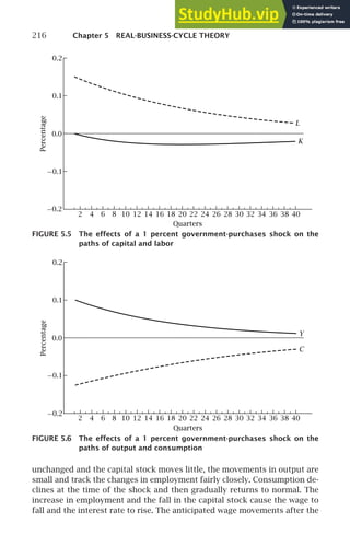
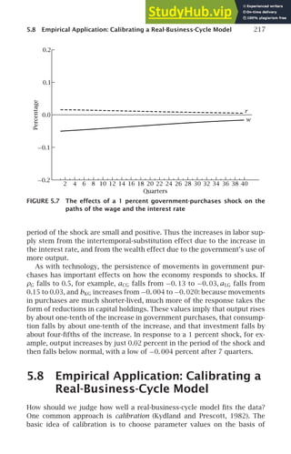
![218 Chapter 5 REAL-BUSINESS-CYCLE THEORY
microeconomic evidence and then to compare the model’s predictions con-
cerning the variances and covariances of various series with those in the
data.
Calibration has two potential advantages over estimating models econo-
metrically. First, because parameter values are selected on the basis of mi-
croeconomic evidence, a large body of information beyond that usually em-
ployed can be brought to bear, and the models can therefore be held to a
higher standard. Second, the economic importance of a statistical rejection,
or lack of rejection, of a model is often hard to interpret. A model that fits
the data well along every dimension except one unimportant one may be
overwhelmingly rejected statistically. Or a model may fail to be rejected
simply because the data are consistent with a wide range of possibilities.
To see how calibration works in practice, consider the baseline real-
business-cycle model of Prescott (1986) and Hansen (1985). This model dif-
fers from the model we have been considering in two ways. First, govern-
ment is absent. Second, the trend component of technology is not assumed
to follow a simple linear path; instead, a smooth but nonlinear trend is re-
moved from the data before the model’s predictions and actual fluctuations
are compared.23
We consider the parameter values proposed by Hansen and Wright (1992),
which are similar to those we considered in the previous section as well as
those considered by Hansen and Wright. Based on data on factor shares, the
capital-output ratio, and the investment-output ratio, Hansen and Wright
set α = 0.36, δ = 2.5% per quarter, and ρ = 1% per quarter. Based on
the average division of discretionary time between work and nonwork ac-
tivities, they set b to 2. They choose the parameters of the process for
technology on the basis of the empirical behavior of the Solow residual,
Rt ≡ ln Yt − [α ln Kt + (1 − α) ln Lt]. As described in Chapter 1, the
Solow residual is a measure of all influences on output growth other than the
contributions of capital and labor through their private marginal products.
Under the assumptions of real-business-cycle theory, the only such other in-
fluence on output is technology, and so the Solow residual is a measure of
technological change. Based on the behavior of the Solow residual, Hansen
and Wright set ρA = 0. 95 and the standard deviation of the quarterly εA ’s
to 1.1 percent.24
Table 5.4 shows the model’s implications for some key features of fluc-
tuations. The figures in the first column are from actual U.S. data; those in
23
The detrending procedure that is used is known as the Hodrick–Prescott filter (Hodrick
and Prescott, 1997).
24
In addition, Prescott argues that, under the assumption that technology multiplies an
expression of form F (K,L), the absence of a strong trend in capital’s share suggests that F (•)
is approximately Cobb–Douglas. Similarly, he argues on the basis of the lack of a trend in
leisure per person and of studies of substitution between consumption in different periods
that (5.7) provides a good approximation to the instantaneous utility function. Thus the
choices of functional forms are not arbitrary.](https://image.slidesharecdn.com/advanced-macroeconomics-230806183016-1212def2/85/Advanced-Macroeconomics-240-320.jpg)
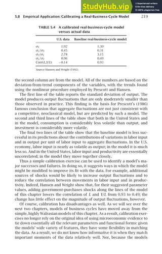

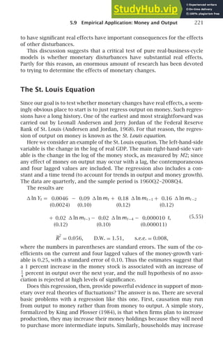


![230 Chapter 5 REAL-BUSINESS-CYCLE THEORY
from leisure in period t is b ln [1 − (Lt/Nt )]. This expression has a negative
second derivative with respect to Lt: there is increasing marginal disutility of
working. As a result, Lt varies less in response to a given amount of variation
in wages in the conventional version of the model than in the indivisible-
labor version. Hansen and Wright (1992) report that introducing indivisible
labor into the Prescott model discussed in Section 5.8 raises the standard
deviation of output from 1.30 to 1.73 percent (versus 1.92 percent in the
data), and the ratio of the standard deviation of total hours to the standard
deviation of output from 0.49 to 0.76 (versus 0.96 in the data).31
A second major extension is to include distortionary taxes (see Green-
wood and Huffman, 1991; Baxter and King, 1993; Campbell, 1994; Braun,
1994; and McGrattan, 1994). A particularly appealing case is proportional
output taxation, so Tt = τtYt, where τt is the tax rate in period t. Output
taxation corresponds to equal tax rates on capital and labor, which is a
reasonable first approximation for many countries. With output taxation,
a change in 1 − τ is, from the point of view of private agents, just like a
change in technology, A1−α
: it changes the amount of output they obtain
from a given amount of capital and labor. Thus for a given process for 1−τ,
after-tax output behaves just as total output does in a model without tax-
ation in which A1−α
follows that same process. This makes the analysis of
distortionary taxation straightforward (Campbell, 1994).
Since tax revenues are used to finance government purchases, it is natural
to analyze the effects of distortionary taxation and government purchases
together. Doing this can change our earlier analysis of the effects of gov-
ernment purchases significantly. Most importantly, predictable changes in
marginal tax rates create additional intertemporal-substitution effects that
can be quantitatively important. For example, in response to a temporary
increase in government purchases financed by a temporary increase in dis-
tortionary taxation, the tax-induced incentives for intertemporal substitu-
tion typically outweigh the other forces affecting output, so that aggregate
output falls rather than rises (Baxter and King, 1993).
Another important extension of real models of fluctuations is the inclu-
sion of multiple sectors and sector-specific shocks. Long and Plosser (1983)
develop a multisector model similar to the model of Section 5.5 and inves-
tigate its implications for the transmission of shocks among sectors. Lilien
(1982) proposes a distinct mechanism through which sectoral technology or
relative-demand shocks can cause employment fluctuations. The basic idea
is that if the reallocation of labor across sectors is time-consuming, em-
ployment falls more rapidly in the sectors suffering negative shocks than
it rises in the sectors facing favorable shocks. As a result, sector-specific
31
Because the instantaneous utility function, (5.7), is separable between consumption
and leisure, expected utility is maximized when employed and unemployed workers have
the same consumption. Thus the indivisible-labor model implies that the unemployed are
better off than the employed. See Problem 10.6 and Rogerson and Wright (1988).](https://image.slidesharecdn.com/advanced-macroeconomics-230806183016-1212def2/85/Advanced-Macroeconomics-252-320.jpg)


![234 Chapter 5 REAL-BUSINESS-CYCLE THEORY
5.5. Consider the problem investigated in (5.16)–(5.21).
(a) Show that an increase in both w1 and w2 that leaves w1/w2 unchanged
does not affect ℓ1 or ℓ2.
(b) Now assume that the household has initial wealth of amount Z 0.
(i) Does (5.23) continue to hold? Why or why not?
(ii) Does the result in (a) continue to hold? Why or why not?
5.6. Suppose an individual lives for two periods and has utility ln C1 + ln C2.
(a) Suppose the individual has labor income of Y1 in the first period of life
and zero in the second period. Second-period consumption is thus
(1 + r)(Y1 − C1); r, the rate of return, is potentially random.
(i) Find the first-order condition for the individual’s choice of C1.
(ii) Suppose r changes from being certain to being uncertain, without any
change in E[r]. How, if at all, does C1 respond to this change?
(b) Suppose the individual has labor income of zero in the first period and
Y2 in the second. Second-period consumption is thus Y2 − (1 + r)C1. Y2 is
certain; again, r may be random.
(i) Find the first-order condition for the individual’s choice of C1.
(ii) Suppose r changes from being certain to being uncertain, without any
change in E[r]. How, if at all, does C1 respond to this change?
5.7. (a) Use an argument analogous to that used to derive equation (5.23) to show
that household optimization requires b/(1 − ℓt) = e−ρ
Et [wt(1 + rt +1)b/
wt +1(1 − ℓt +1)] .
(b) Show that this condition is implied by (5.23) and (5.26). (Note that [5.26]
must hold in every period.)
5.8. A simplified real-business-cycle model with additive technology shocks.
(This follows Blanchard and Fischer, 1989, pp. 329–331.) Consider an econ-
omy consisting of a constant population of infinitely lived individuals. The
representative individual maximizes the expected value of
∞
t=0
u(Ct)/(1 + ρ)t
,
ρ 0. The instantaneous utility function, u(Ct), is u(Ct) = Ct − θC 2
t , θ 0.
Assume that C is always in the range where u′
(C) is positive.
Output is linear in capital, plus an additive disturbance: Yt = AKt + et.
There is no depreciation; thus Kt +1 = Kt + Yt − Ct, and the interest rate is A.
Assume A = ρ. Finally, the disturbance follows a first-order autoregressive
process: et = φet −1 + εt, where −1 φ 1 and where the εt’s are mean-zero,
i.i.d. shocks.
(a) Find the first-order condition (Euler equation) relating Ct and expectations
of Ct +1.
(b) Guess that consumption takes the form Ct = α + βKt + γ et. Given this
guess, what is Kt +1 as a function of Kt and et?
(c) What values must the parameters α, β, and γ have for the first-order con-
dition in part (a) to be satisfied for all values of Kt and et?](https://image.slidesharecdn.com/advanced-macroeconomics-230806183016-1212def2/85/Advanced-Macroeconomics-256-320.jpg)
![Problems 235
(d) What are the effects of a one-time shock to ε on the paths of Y, K,
and C ?
5.9. A simplified real-business-cycle model with taste shocks. (This follows
Blanchard and Fischer, 1989, p. 361.) Consider the setup in Problem 5.8. As-
sume, however, that the technological disturbances (the e’s) are absent and
that the instantaneous utility function is u(Ct ) = Ct − θ(Ct + νt )2
. The ν’s are
mean-zero, i.i.d. shocks.
(a) Find the first-order condition (Euler equation) relating Ct and expectations
of Ct +1.
(b) Guess that consumption takes the form Ct = α + βKt + γ νt. Given this
guess, what is Kt +1 as a function of Kt and νt?
(c) What values must the parameters α, β, and γ have for the first-order con-
dition in (a) to be satisfied for all values of Kt and νt?
(d) What are the effects of a one-time shock to ν on the paths of Y, K, and C ?
5.10. The balanced growth path of the model of Section 5.3. Consider the model
of Section 5.3 without any shocks. Let y∗, k∗, c∗, and G∗ denote the values
of Y/(AL), K/(AL), C/(AL), and G/(AL) on the balanced growth path; w∗ the
value of w/A; ℓ ∗ the value of L/N; and r∗ the value of r.
(a) Use equations (5.1)–(5.4), (5.23), and (5.26) and the fact that y∗, k∗, c∗, w∗,
ℓ ∗, and r∗ are constant on the balanced growth path to find six equations
in these six variables. (Hint: The fact that c in [5.23] is consumption per
person, C/N, and c∗ is the balanced-growth-path value of consumption
per unit of effective labor, C/(AL), implies that c = c∗ℓ ∗A on the balanced
growth path.)
(b) Consider the parameter values assumed in Section 5.7. What are the im-
plied shares of consumption and investment in output on the balanced
growth path? What is the implied ratio of capital to annual output on the
balanced growth path?
5.11. Solving a real-business-cycle model by finding the social optimum.34
Con-
sider the model of Section 5.5. Assume for simplicity that n = g = A = N =
0. Let V(Kt,At), the value function, be the expected present value from the
current period forward of lifetime utility of the representative individual as
a function of the capital stock and technology.
(a) Explain intuitively why V (•) must satisfy
V(Kt,At) = max
Ct,ℓt
{[ln Ct + b ln(1 − ℓt)] + e−ρ
Et [V(Kt +1,At +1)]}.
This condition is known as the Bellman equation.
Given the log-linear structure of the model, let us guess that V (•) takes
the form V(Kt,At) = β0 + βK ln Kt + βA ln At, where the values of the β’s
are to be determined. Substituting this conjectured form and the facts
34
This problem uses dynamic programming and the method of undetermined coeffi-
cients. These two methods are explained in Section 10.4 and Section 5.6, respectively.](https://image.slidesharecdn.com/advanced-macroeconomics-230806183016-1212def2/85/Advanced-Macroeconomics-257-320.jpg)
![236 Chapter 5 REAL-BUSINESS-CYCLE THEORY
that Kt +1 = Yt − Ct and Et [ln At +1] = ρA ln At into the Bellman equation
yields
V(Kt,At) = max
Ct,ℓt
{[ln Ct +b ln(1−ℓt)]+e−ρ
[β0 +βK ln(Yt −Ct)+βA ρA ln At]}.
(b) Find the first-order condition for Ct. Show that it implies that Ct/Yt does
not depend on Kt or At.
(c) Find the first-order condition for ℓt. Use this condition and the result in
part (b) to show that ℓt does not depend on Kt or At.
(d) Substitute the production function and the results in parts (b) and (c) for
the optimal Ct and ℓt into the equation above for V(•), and show that the
resulting expression has the form V(Kt,At) = β′
0 + β′
K ln Kt + β′
A ln At.
(e) What must βK and βA be so that β′
K = βK and β′
A = βA ?35
(f) What are the implied values of C/Y and ℓ? Are they the same as those
found in Section 5.5 for the case of n = g = 0?
5.12. Suppose technology follows some process other than (5.8)–(5.9). Do st = ŝ
and ℓt = ℓ̂ for all t continue to solve the model of Section 5.5? Why or
why not?
5.13. Consider the model of Section 5.5. Suppose, however, that the instantaneous
utility function, ut, is given by ut = ln ct + b(1 − ℓt )1−γ
/(1 − γ ), b 0, γ 0,
rather than by (5.7) (see Problem 5.4).
(a) Find the first-order condition analogous to equation (5.26) that relates
current leisure and consumption, given the wage.
(b) With this change in the model, is the saving rate (s) still constant?
(c) Is leisure per person (1 − ℓ) still constant?
5.14. (a) If the Ãt’s are uniformly 0 and if ln Yt evolves according to (5.39), what
path does ln Yt settle down to? (Hint: Note that we can rewrite [5.39] as
ln Yt − (n + g)t = Q + α[ln Yt −1 − (n + g)(t − 1)] + (1 − α)Ãt, where Q ≡
α ln ŝ + (1 − α)(A + ln ℓ̂ + N ) − α(n + g).)
(b) Let Ỹ t denote the difference between ln Yt and the path found in (a). With
this definition, derive (5.40).
5.15. The derivation of the log-linearized equation of motion for capital. Con-
sider the equation of motion for capital, Kt +1 = Kt + Kα
t (At Lt)1−α
− Ct −
Gt − δKt.
(a) (i) Show that ∂ ln Kt +1/∂ ln Kt (holding At, Lt, Ct, and Gt fixed) equals
(1 + rt +1)(Kt/Kt +1).
(ii) Show that this implies that ∂ ln Kt +1/∂ ln Kt evaluated at the balanced
growth path is (1 + r∗)/en+g
.36
35
The calculation of β0 is tedious and is therefore omitted.
36
One could express r ∗ in terms of the discount rate ρ. Campbell (1994) argues, however,
that it is easier to discuss the model’s implications in terms of r ∗ than ρ.](https://image.slidesharecdn.com/advanced-macroeconomics-230806183016-1212def2/85/Advanced-Macroeconomics-258-320.jpg)


![6.1 A Baseline Case: Fixed Prices 239
see, are almost certainly small—can lead to substantial aggregate nominal
rigidity.
Part A Exogenous Nominal Rigidity
6.1 A Baseline Case: Fixed Prices
In this part of the chapter, we take nominal rigidity as given and investi-
gate its effects. We begin with the extreme case where nominal prices are
not just less than fully flexible, but completely fixed. Aside from this ex-
ogenously imposed assumption of price rigidity, the model is built up from
microeconomic foundations.
Assumptions
Time is discrete. Firms produce output using labor as their only input. Ag-
gregate output is therefore given by
Y = F (L), F ′
(•) 0, F ′′
(•) ≤ 0. (6.1)
Government and international trade are absent from the model. Together
with the assumption that there is no capital, this implies that aggregate
consumption and aggregate output are equal.
There is a fixed number of infinitely lived households that obtain utility
from consumption and from holding real money balances, and disutility
from working. For simplicity, we ignore population growth and normalize
the number of households to 1. The representative household’s objective
function is
U =
∞
t=0
βt
[U(Ct) + ⌫
Mt
Pt
− V(Lt)], 0 β 1. (6.2)
There is diminishing marginal utility of consumption and money holdings,
and increasing marginal disutility of working: U′
(•) 0, U′′
(•) 0, ⌫
′
(•) 0,
⌫
′′
(•) 0, V′
(•) 0, V′′
(•) 0. We assume that U(•) and ⌫(•) take our usual
constant-relative-risk-aversion forms:
U(Ct) =
C1−θ
t
1 − θ
, θ 0, (6.3)
⌫
Mt
Pt
=
(Mt/Pt)1−ν
1 − ν
, ν 0. (6.4)
The assumption that money is a direct source of utility is a shortcut.
In truth, individuals hold cash not because it provides utility directly, but](https://image.slidesharecdn.com/advanced-macroeconomics-230806183016-1212def2/85/Advanced-Macroeconomics-261-320.jpg)
![6.1 A Baseline Case: Fixed Prices 241
Taking logs of both sides and solving for ln Ct gives us
ln Ct = ln Ct+1 −
1
θ
ln[(1 + rt)β]. (6.7)
To get this expression into a form that is more useful, we make three
changes. First, and most importantly, recall that the only use of output is
for consumption and that we have normalized the number of households
to 1. Thus in equilibrium, aggregate output, Y, and the consumption of the
representative household, C, must be equal. We therefore substitute Y for
C. Second, for small values of r, ln(1 + r) ≈ r. For simplicity, we treat this
relationship as exact. And third, we suppress the constant term, −(1/θ) ln β.3
These changes give us:
ln Yt = ln Yt+1 −
1
θ
rt. (6.8)
Equation (6.8) is known as the new Keynesian IS curve. In contrast to
the traditional IS curve, it is derived from microeconomic foundations. The
main difference from the traditional IS curve is the presence of Yt+1 on the
right-hand side.4
For our purposes, the most important feature of the new Keynesian IS
curve is that it implies an inverse relationship between rt and Yt. More elab-
orate analyses of the demand for goods have the same implication. For ex-
ample, we will see in Chapter 9 that increases in the real interest rate reduce
the amount of investment firms want to undertake. Thus adding capital to
the model would introduce another reason for a downward-sloping relation-
ship. Similarly, suppose we introduced international trade. A rise in the
country’s interest rate would generally increase demand for the country’s
assets, and so cause its exchange rate to appreciate. This in turn would
reduce exports and increase imports.
To find the first-order condition for households’ money holdings, con-
sider a balanced-budget change in Mt/Pt and Ct. Specifically, suppose the
household raises Mt/Pt by dm and lowers Ct by [it/(1 + it)]dm. The house-
hold’s real bond holdings therefore fall by {1 − [it/(1 + it)]}dm, or [1/(1 +
it)]dm. This change has no effect on the household’s wealth at the begin-
ning of period t + 1. Thus if the household is optimizing, at the margin this
change must not affect utility.
The utility benefit of the change is ⌫
′
(Mt/Pt)dm, and the utility cost is
U′
(Ct)[it/(1 + it)]dm. The first-order condition for optimal money holdings
3
This can be formalized by reinterpreting r as the difference between the real interest
rate and − ln β.
4
The new Keynesian IS curve is derived by Kerr and King (1996) and McCallum and
Nelson (1999). Under uncertainty, with appropriate assumptions ln Yt+1 can be replaced with
Et[ln Yt+1] plus a constant.](https://image.slidesharecdn.com/advanced-macroeconomics-230806183016-1212def2/85/Advanced-Macroeconomics-263-320.jpg)
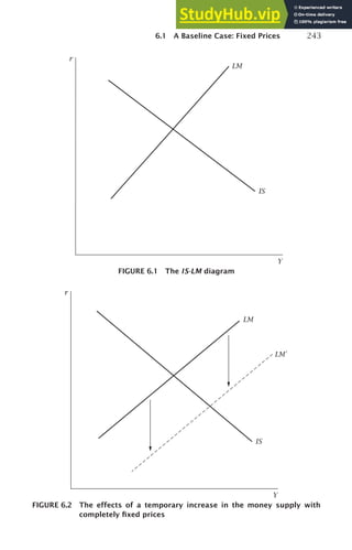

![6.2 Alternative Assumptions about Price and Wage Rigidity 245
pricing behavior, and the behavior of the real wage and the markup in re-
sponse to demand fluctuations.
We consider four sets of assumptions. The first two are valuable base-
lines. Both, however, appear to fail as even remotely approximate descrip-
tions of actual economies. The other two are more complicated and poten-
tially more accurate. Together, the four cases illustrate the wide range of
possibilities.
Case 1: Keynes’s Model
The supply side of the model in Keynes’s General Theory (1936) has two
key features. First, the nominal wage is completely unresponsive to current-
period developments (at least over some range):
W = W. (6.12)
(Throughout this section, we focus on the economy in a single period. Thus
we omit time subscripts for simplicity.) Second, for reasons that Keynes did
not specify explicitly, the wage that prevails in the absence of nominal rigid-
ity is above the level that equates supply and demand. Thus, implicitly, the
labor market has some non-Walrasian feature that causes the equilibrium
real wage to be above the market-clearing level.
Keynes’s assumptions concerning the goods market, in contrast, are con-
ventional. As in Section 6.1, output is given by Y = F (L), with F′
(•) 0 and
F ′′
(•) ≤ 0 (see equation [6.1]). Firms are competitive and their prices are
flexible, and so they hire labor up to the point where the marginal product
of labor equals the real wage:
F ′
(L) =
W
P
. (6.13)
With these assumptions, an increase in demand raises output through its
impact on the real wage. When the money supply or some other determinant
of demand rises, goods prices rise, and so the real wage falls and employ-
ment rises. Because the real wage is initially above the market-clearing level,
workers are willing to supply the additional labor.
Figure 6.3 shows the situation in the labor market. The initial level of em-
ployment is determined by labor demand and the prevailing real wage (Point
E in the diagram). Thus there is involuntary unemployment: some workers
would like to work at the prevailing wage but cannot. The amount of un-
employment is the difference between supply and demand at the prevailing
real wage (distance EA in the diagram).
Fluctuations in the demand for goods lead to movements of employment
and the real wage along the downward-sloping labor demand curve. Higher
demand, for example, raises the price level. Thus it leads to a lower real
wage and higher employment. This is shown as Point E′
in the diagram. This](https://image.slidesharecdn.com/advanced-macroeconomics-230806183016-1212def2/85/Advanced-Macroeconomics-267-320.jpg)
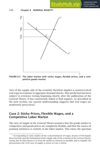
![6.2 Alternative Assumptions about Price and Wage Rigidity 247
of what occurs in the reverse case where the labor market is competitive and
wages are completely flexible, and where the source of incomplete nominal
adjustment is entirely in the goods market.
In the previous case, we assumed that in the absence of nominal rigidity,
the wage is above the market-clearing level. This assumption was neces-
sary for increases in demand to lead to higher employment. Likewise, when
the nominal rigidity is in the goods market, we assume that the flexible-
price equilibrium involves prices that exceed marginal costs. Without this
assumption, if the demand for goods rose, firms would turn customers away
rather than meet the additional demand at their fixed prices.
Models of nominal rigidity in the goods market almost always assume
that the reason prices normally exceed marginal costs is that firms have
market power, so that profit-maximizing prices are above marginal costs.
Under this assumption, at the flexible-price equilibrium, firms are better off
if they can sell more at the prevailing price. As a result, a rise in demand
with rigid prices leads to higher output.
When prices rather than wages are assumed rigid, the assumption from
Section 6.1 that P = P (equation [6.11]), which we dropped in Case 1, again
applies. Wages are flexible and the labor market is competitive. Thus work-
ers choose their labor supply to maximize utility taking the real wage as
given. From the utility function, (6.2)–(6.4), the first-order condition for op-
timal labor supply is
C−θ W
P
= V ′
(L). (6.14)
In equilibrium, C = Y = F (L). Thus (6.14) implies
W
P
= [F (L)]θ
V ′
(L). (6.15)
The right-hand side of this expression is increasing in L. Thus (6.15) implic-
itly defines L as an increasing function of the real wage:
L = Ls
W
P
, Ls ′
(•) 0. (6.16)
Finally, firms meet demand at the prevailing price as long as it does not
exceed the level where marginal cost equals price.
With these assumptions, fluctuations in demand cause firms to change
employment and output at the fixed price level. Figure 6.4 shows the model’s
implications for the labor market. Firms’ demand for labor is determined
by their desire to meet the demand for their goods. Thus, as long as the
real wage is not so high that it is unprofitable to meet the full demand, the
labor demand curve is a vertical line in employment-wage space. The term
effective labor demand is used to describe a situation, such as this, where the](https://image.slidesharecdn.com/advanced-macroeconomics-230806183016-1212def2/85/Advanced-Macroeconomics-269-320.jpg)
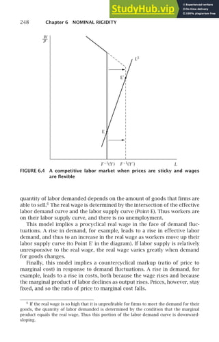

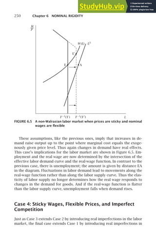
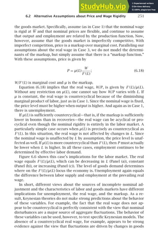
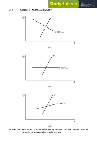


![256 Chapter 6 NOMINAL RIGIDITY
discusses how one can modify the models to turn them into a potentially
helpful framework for thinking about real-world issues. We will begin with
the supply side, and then turn to the demand side.
A Permanent Output-Inflation Tradeoff?
To build a model we would want to use in practice, we need to relax the
assumption that nominal prices or wages never change. One natural way to
do this is to suppose that the level at which current prices or wages are fixed
is determined by what happened the previous period. Consider, for example,
our first model of supply; this is the model with fixed wages, flexible prices,
and a competitive goods market.9
Suppose, however, that rather than being
an exogenous parameter, W is proportional to the previous period’s price
level. That is, suppose that wages are adjusted to make up for the previous
period’s inflation:
Wt = APt −1, A 0, (6.20)
Recall that in our first model of supply, employment is determined by
F ′
(Lt) = Wt/Pt (equation [6.13]). Equation (6.20) for Wt therefore implies
F ′
(Lt) =
APt −1
Pt
(6.21)
=
A
1 + πt
,
where πt is the inflation rate. Equation (6.21) implies a stable, upward-
sloping relationship between employment (and hence output) and inflation.
That is, it implies that there is a permanent output-inflation tradeoff: by
accepting higher inflation, policymakers can permanently raise output. And
since higher output is associated with lower unemployment, it also implies
a permanent unemployment-inflation tradeoff.
In a famous paper, Phillips (1958) showed that there was in fact a strong
and relatively stable negative relationship between unemployment and wage
inflation in the United Kingdom over the previous century. Subsequent
researchers found a similar relationship between unemployment and price
inflation—a relationship that became known as the Phillips curve. Thus
there appeared to be both theoretical and empirical support for a stable
unemployment-inflation tradeoff.
9
The other models of Section 6.2 could be modified in similar ways, and would have
similar implications.](https://image.slidesharecdn.com/advanced-macroeconomics-230806183016-1212def2/85/Advanced-Macroeconomics-278-320.jpg)


![6.4 Toward a Usable Model with Exogenous Nominal Rigidity 261
may depend on the environment: how rapidly core inflation adjusts to
changes in inflation is likely to depend on how long-lasting actual move-
ments in inflation typically are. If this is right, then in a situation like the
one that Phillips studied, where there are many transitory movements in in-
flation, core inflation will vary little; the data will therefore suggest a stable
relationship between output and inflation. But in a setting like the United
States in the 1970s and 1980s, where there are sustained periods of high
and of low inflation, core inflation will vary more, and thus there will be no
consistent link between output and the level of inflation.
Carrying these criticisms of (6.22)–(6.23) to their logical extreme would
suggest that we replace core inflation in (6.22) with expected inflation:
πt = πe
t + λ(ln Yt − ln Yt ) + εS
t , (6.24)
where πe
t is expected inflation. This formulation captures the ideas in the
previous examples. For example, (6.24) implies that unless expectations are
grossly irrational, no policy can permanently raise output above its natural
rate, since that requires that workers’ and firms’ forecasts of inflation are
always too low. Similarly, since expectations of future inflation respond less
to current inflation when movements in inflation tend to be shorter-lived,
(6.24) is consistent with Friedman’s example of how the output-inflation
relationship is likely to vary with the behavior of actual inflation.
Nonetheless, practical modern formulations of pricing behavior gener-
ally do not use the model of supply in (6.24). The central reason is that, as
we will see in Section 6.9, if one assumes that price- and wage-setters are
rational in forming their expectations, then (6.24) has strong implications—
implications that do not appear to be supported by the data. Alternatively,
if one assumes that workers and firms do not form their expectations ratio-
nally, one is resting the theory on irrationality.
A natural compromise between the models of core inflation in (6.23) and
in (6.24) is to assume that core inflation is a weighted average of past infla-
tion and expected inflation. With this assumption, we have a hybrid Phillips
curve:
πt = φπe
t + (1 − φ)πt −1 + λ(ln Yt − ln Yt ) + εS
t , 0 ≤ φ ≤ 1. (6.25)
As long as φ is strictly less than 1, there is some inertia in wage and price
inflation. That is, there is some link between past and future inflation be-
yond effects operating through expectations. We will return to this issue in
the next chapter.
Aggregate Demand, Aggregate Supply, and the AS-AD
Diagram
Our simple formulation of the demand side of the economy in Section 6.1
had two elements: the new Keynesian IS curve, ln Yt = E[ln Yt+1] − 1
θ
rt](https://image.slidesharecdn.com/advanced-macroeconomics-230806183016-1212def2/85/Advanced-Macroeconomics-283-320.jpg)
![262 Chapter 6 NOMINAL RIGIDITY
(equation [6.8]), and the LM curve, Mt/Pt = Yθ/ν
t [(1+ it)/it]1/ν
(equation [6.10]).
Coupled with the assumption that Mt was set exogenously by the central
bank, these equations led to the IS-LM diagram in (Y,r) space
(Figure 6.1).
The ideas captured by the new Keynesian IS curve are appealing and use-
ful: increases in the real interest rate reduce the current demand for goods
relative to future demand, and increases in expected future income raise
current demand. The LM curve, in contrast, is quite problematic in practical
applications. One difficulty is that the model becomes much more compli-
cated once we relax Section 6.1’s assumption that prices are permanently
fixed; changes in either Pt or πe
t shift the LM curve in (Y,r) space. A second
difficulty is that modern central banks do not focus on the money supply.
An alternative approach that avoids the difficulties with the LM curve is
to assume that the central bank conducts policy in terms of a rule for the
interest rate (Taylor, 1993; Bryant, Hooper, and Mann, 1993). We will discuss
such interest-rate rules extensively in our examination of monetary policy
in Chapter 11. For now, however, we simply assume that the central bank
conducts policy so as to make the real interest rate an increasing function
of the gap between actual and potential output and of inflation:
rt = r(ln Yt − ln Yt,πt), r1(•) 0,r2(•) 0. (6.26)
The way the central bank carries out this policy is by adjusting the money
supply to make (6.26) hold. That is, it sets the money supply at t so that
the money market equilibrium condition, which we can write as
Mt
Pt
= Yθ/ν
t [(1 + rt + πe
t )/(rt + πe
t )]1/ν
yields the value of rt that satisfies (6.26).
For most purposes, however, we can neglect the money market and work
directly with (6.26).
The central bank’s interest-rate rule, (6.26), directly implies an upward-
sloping relationship between Yt and rt (for a given value of πt). This rela-
tionship is known as the MP curve. It is shown together with the IS curve in
Figure 6.8.
The determination of output and inflation can then be described by two
curves in output-inflation space, an upward-sloping aggregate supply (AS)
curve and a downward-sloping aggregate demand (AD) curve. The AS curve
follows directly from (6.22), πt = π∗
t + λ(ln Yt − ln Yt) + εS
t . The AD curve
comes from the IS and MP curves. To see this, consider a rise in infla-
tion. Since π does not enter households’ intertemporal first-order condi-
tion, (6.7), the IS curve is unaffected. But since the monetary-policy rule,
r = r(ln Y − ln Y,π), is increasing in π, the rise in inflation increases the real
interest rate the central bank sets at a given level of output. That is, the MP
curve shifts up. As a result, r rises and Y falls. Thus the level of output at the
intersection of the IS and MP curves is a decreasing function of inflation.
The AS and AD curves are shown in Figure 6.9.](https://image.slidesharecdn.com/advanced-macroeconomics-230806183016-1212def2/85/Advanced-Macroeconomics-284-320.jpg)

![264 Chapter 6 NOMINAL RIGIDITY
Example: IS Shocks
We now have a three-equation model: the new Keynesian IS curve, the MP
curve, and the AS curve. A common approach to obtaining a model one can
work with is to assume that core inflation, π∗
t , is given by lagged inflation,
πt −1, as in (6.23), and that the MP curve is linear. Even then, however, the
conjunction of forward-looking elements (from the Et[ln Yt+1] term in the
IS curve) and backward-looking ones (from the πt −1 term in the AS curve)
makes solving the model complicated.
A solution to this difficulty that is somewhat arbitrary but nonetheless
often useful is to simply drop the Et[ln Yt+1] term from the IS curve. The
result is the traditional IS curve, where output depends negatively on the
real interest rate and is not affected by any other endogenous variables.
The attractiveness of this approach is that it makes the model very easy to
solve. There is no need to assume linear functional forms; shocks to any
of the equations can be considered without making assumptions about the
processes followed by the shocks; and the analysis can be done graphi-
cally. For these reasons, this approach is often useful and is the standard
approach in undergraduate teaching.
At the same time, however, the logic of the model implies that the ex-
pected output term belongs in the IS equation, and thus that it is desirable
to understand the implications of the full model. To get a feel for this,
here we consider a very stripped-down version. Crucially, we assume that
the monetary-policy rule depends only on output and not on inflation; this
assumption eliminates the backward-looking element of output behavior.
Second, we assume that the only shocks are to the IS curve, and that the
shocks follow a first-order autoregressive process. Finally, we make several
minor assumptions to simplify the notation and presentation: ln Yt is zero
for all t, the MP equation is linear, the constant term in the MP equation is
zero, and yt denotes ln Yt.
These assumptions give us the system:
πt = πt −1 + λyt, λ 0, (6.27)
rt = byt, b 0, (6.28)
yt = Et[yt +1] −
1
θ
rt + uI S
t , θ 0, (6.29)
uI S
t = ρI SuI S
t −1 + eI S
t , −1 ρI S 1, (6.30)
where eI S
is white noise. Equation (6.27) is the AS curve, (6.28) is the MP
curve, (6.29) is the IS curve, and (6.30) describes the behavior of the IS
shocks.](https://image.slidesharecdn.com/advanced-macroeconomics-230806183016-1212def2/85/Advanced-Macroeconomics-286-320.jpg)
![6.4 Toward a Usable Model with Exogenous Nominal Rigidity 265
We can combine (6.28) and (6.29) and use straightforward algebra to solve
for yt in terms of uI S
t and Et[yt +1]:
yt =
θ
θ + b
Et[yt +1] +
θ
θ + b
uI S
t
(6.31)
≡ φEt[yt +1] + φuI S
t ,
where φ = θ/(θ + b). Note that our assumptions imply 0 φ 1.
Equation (6.31) poses a challenge: it expresses y in terms of not just the
disturbance, uI S
t , but the expectation of the future value of an endogenous
variable, Et[yt +1]. Thus it is not immediately clear how to trace out the effect
of a shock. To address this problem, note that (6.31) holds in all future
periods:
yt +j = φEt +j[yt +j +1] + φuI S
t +j for j = 1, 2, 3, . . . (6.32)
Taking expectations of both sides of (6.32) as of time t implies
Et[yt +j] = φEt[yt +j +1] + φρ
j
I SuI S
t . (6.33)
Equation (6.33) uses the fact that Et[Et +j[yt +j +1]] is simply Et[yt +j +1]; oth-
erwise agents would be expecting to revise their estimate of yt +j +1 either up
or down, which would imply that their original estimate was not rational.
The fact that the current expectation of a future expectation of a variable
equals the current expectation of the variable is known as the law of iterated
projections.
We can now iterate (6.31) forward. That is, we first express Et[yt +1] in
terms of Et[yt +2] and Et[uI S
t +1]; we then express Et[yt +2] in terms of Et[yt +3]
and Et[uI S
t +2]; and so on. Doing this gives us:
yt = φuI S
t + φ
φEt[yt +2] + φρI SuI S
t
= φuI S
t + φ2
ρI SuI S
t + φ2
φEt[yt +3] + φρ2
I SuI S
t
= · · · (6.34)
=
φ + φ2
ρI S + φ3
ρ2
I S + · · ·
uI S
t + lim
n →∞
φn
Et[yt +n]
=
φ
1 − φρI S
uI S
t + lim
n →∞
φn
Et[yt +n].
If we assume that limn →∞ φn
Et[yt +n] converges to zero (an issue we will
return to in a moment) and substitute back in for φ, we obtain
yt =
θ
θ + b − θρI S
uI S
t . (6.35)
This expression shows how various forces influence how shocks to de-
mand affect output. For example, a more aggressive monetary-policy](https://image.slidesharecdn.com/advanced-macroeconomics-230806183016-1212def2/85/Advanced-Macroeconomics-287-320.jpg)
![266 Chapter 6 NOMINAL RIGIDITY
response to output movements (that is, a higher value of b) dampens the
effects of shocks to the IS curve.
Observe that in the absence of the forward-looking aspect of the IS curve
(that is, if the IS equation is just yt = −(1/θ)rt + uI S
t ), output is [θ/(θ +
b)]uI S
t . Equation (6.35) shows that accounting for forward-looking behavior
raises the coefficient on uI S
t as long as ρI S 0. That is, forward-looking
consumption behavior magnifies the effects of persistent shocks to demand.
Equation (6.35) for output and the AS equation, (6.27), imply that inflation
is given by
πt = πt −1 +
θλ
θ + b − θρI S
uI S
t . (6.36)
Because there is no feedback from inflation to the real interest rate, there
is no force acting to stabilize inflation. Indeed, if the shocks to the IS curve
are positively serially correlated, the change in inflation is positively serially
correlated.
The solution for yt in (6.34) includes the term limn →∞ φn
Et[yt +n], which
thus far we have been assuming converges to zero. Since φ is less than one,
this term could fail to converge only if Et[yt +n] diverged. That is, agents
would have to expect y to diverge, which cannot happen. Thus assuming
limn →∞ φn
Et[yt +n] = 0 is appropriate.
One other aspect of this example is worth noting. Suppose φ 1 but
φρI S 1. φ 1 could arise if the central bank followed the perverse policy
of cutting the real interest rate in response to increases in output (so that
b was negative). With φρI S 1, the sum in equation (6.34) still converges,
and so that expression is still correct. And if (6.35) holds, limn →∞ φn
Et[yt +n]
equals limn →∞ φn
ρn
I S[θ/(θ + b − θρI S)]uI S
t , which is zero. That is, although
one might expect φ 1 to generate instability, the conventional solution to
the model still carries over to this case as long as φρI S 1.
Interestingly, however, this is now no longer the only solution. If φ ex-
ceeds 1, then limn →∞ φn
Et[yt +n] can differ from zero without Et[yt +n] di-
verging. As a result, there can be spontaneous, self-fulfilling changes in the
path of output. To see this, suppose that uI S
t = 0 for all t and that initially
yt = 0 for all t. Now suppose that in some period, which we will call period
0, y rises by some amount X—not because of a change in tastes, govern-
ment purchases, or some other external influence (that is, not because of a
nonzero realization of uI S
0 ), but simply because a change in agents’ beliefs
about the equilibrium path of the economy. If agents’ expectation of yt is
X/φt
for t ≥ 0, they will act in ways that make their expectations correct.
That is, this change can be self-fulfilling.
When the economy has multiple equilibria in this way, the solution with-
out spontaneous, self-fulfilling output movements is known as the funda-
mental solution. Solutions with self-fulfilling output movements are known
as sunspot solutions. Although here the assumption that leads to the possi-
bility of a sunspot solution is contrived, there are many models where this](https://image.slidesharecdn.com/advanced-macroeconomics-230806183016-1212def2/85/Advanced-Macroeconomics-288-320.jpg)

![268 Chapter 6 NOMINAL RIGIDITY
discusses other possible sources of incomplete nominal adjustment. We
will see that the same fundamental issues that arise with menu costs also
arise with other nominal imperfections.
Our goal in this chapter is not to try to construct an even remotely realis-
tic macroeconomic model. For that reason, the models we will consider are
very simple. The next chapter will begin to make the models more realistic
and useful in practical applications.
6.5 A Model of Imperfect Competition
and Price-Setting
Before turning to menu costs and the effects of monetary shocks, we first
examine an economy of imperfectly competitive price-setters with complete
price flexibility. There are two reasons for analyzing this model. First, as
we will see, imperfect competition alone has interesting macroeconomic
consequences. Second, the models in the rest of the chapter are concerned
with the causes and effects of barriers to price adjustment. To address these
issues, we will need a model that shows us what prices firms would choose
in the absence of barriers to adjustment and what happens when prices
depart from those levels.
Assumptions
There is a continuum of differentiated goods indexed by i ∈ [0,1]. Each good
is produced by a single firm with monopoly rights to the production of the
good. Firm i’s production function is just
Yi = Li , (6.37)
where Li is the amount of labor it hires and Yi is its output. Firms hire
labor in a perfectly competitive labor market and sell output in imperfectly
competitive goods markets. In this section, firms can set their prices freely.
They are owned by the households, and so any profits they earn accrue to
the households. As in the model of Section 6.1, we normalize the number
of households to 1.
The utility of the representative household depends positively on its con-
sumption and negatively on the amount of labor it supplies. It takes the
form
U = C −
1
γ
LY
, γ 1. (6.38)
Crucially, C is not the household’s total consumption of all goods. If it were,
goods would be perfect substitutes for one another, and so firms would not](https://image.slidesharecdn.com/advanced-macroeconomics-230806183016-1212def2/85/Advanced-Macroeconomics-290-320.jpg)
![6.5 A Model of Imperfect Competition and Price-Setting 273
where lowercase letters denote the logs of the corresponding uppercase
variables.
We know that each producer charges the same price, and that the price
index, P, equals this common price. Equilibrium therefore requires that each
producer, taking P as given, sets his or her own price equal to P; that is, each
producer’s desired relative price must equal 1. From (6.57), this condition
is [η/(η − 1)]Yγ −1
= 1, or
Y =
η − 1
η
1/(γ −1)
. (6.59)
This is the equilibrium level of output.
Finally, we can use the aggregate demand equation, Y = M/P, to find the
equilibrium price level:
P =
M
Y
=
M
η − 1
η
1/(γ −1)
.
(6.60)
Implications
When producers have market power, they produce less than the socially
optimal amount. To see this, note that in a symmetric allocation each indi-
vidual supplies some amount L of labor, and production of each good and
each individual’s consumption equal that L. Thus the problem of finding the
best symmetric allocation reduces to choosing L to maximize L − (1/γ )L
γ
.
The solution is simply L = 1. As (6.59) shows, equilibrium output is less
than this. Intuitively, the fact that producers face downward-sloping de-
mand curves means that the marginal revenue product of labor is less than
its marginal product. As a result, the real wage is less than the marginal
product of labor: from (6.55) (and the fact that each Pi equals P in equilib-
rium), the real wage is (η − 1)/η; the marginal product of labor, in contrast,
is 1. This reduces the quantity of labor supplied, and thus causes equi-
librium output to be less than optimal. From (6.59), equilibrium output is
[(η − 1)/η]1/(γ −1)
. Thus the gap between the equilibrium and optimal levels
of output is greater when producers have more market power (that is, when
η is lower) and when labor supply is more responsive to the real wage (that
is, when γ is lower).
The fact that equilibrium output is inefficiently low under imperfect com-
petition has important implications for fluctuations. To begin with, it im-
plies that recessions and booms have asymmetric effects on welfare
(Mankiw, 1985). In practice, periods when output is unusually high are
viewed as good times, and periods when output is unusually low are viewed](https://image.slidesharecdn.com/advanced-macroeconomics-230806183016-1212def2/85/Advanced-Macroeconomics-295-320.jpg)
![274 Chapter 6 NOMINAL RIGIDITY
as bad times. But think about an economy where fluctuations arise from
incomplete nominal adjustment in the face of monetary shocks. If the equi-
librium in the absence of shocks is optimal, both times of high output and
times of low output are departures from the optimum, and thus both are un-
desirable. But if equilibrium output is less than optimal, a boom brings out-
put closer to the social optimum, whereas a recession pushes it farther away.
In addition, the gap between equilibrium and optimal output implies that
pricing decisions have externalities. Suppose the economy is initially in equi-
librium, and consider the effects of a marginal reduction in all prices. M/P
rises, and so aggregate output rises. This potentially affects welfare through
two channels. First, the real wage increases (see [6.56]). Since households
employ the same amount of labor in their capacity as owners of the firms
as they supply to the labor market, at the margin this increase does not af-
fect welfare. Second, because aggregate output increases, the demand curve
for each good, Y(Pi /P)−η
, shifts out. Since firms are selling at prices that ex-
ceed marginal costs, this change raises profits, and so increases households’
welfare. Thus under imperfect competition, pricing decisions have external-
ities, and those externalities operate through the overall demand for goods.
This externality is often referred to as an aggregate demand externality
(Blanchard and Kiyotaki, 1987).
The final implication of this analysis is that imperfect competition alone
does not imply monetary nonneutrality. A change in the money stock leads
to proportional changes in the nominal wage and all nominal prices; output
and the real wage are unchanged (see [6.59] and [6.60]).
Finally, since a pricing equation of the form (6.58) is important in later
sections, it is worth noting that the basic idea captured by the equation is
much more general than the specific model of price-setters’ desired prices
we are considering here. Equation (6.58) states that p∗
i − p takes the form
c + φy. That is, it states that a price-setter’s optimal relative price is in-
creasing in aggregate output. In the particular model we are considering,
this arises from increases in the prevailing real wage when output rises. But
in a more general setting, it can also arise from increases in the costs of
other inputs, from diminishing returns, or from costs of adjusting output.
The fact that price-setters’ desired real prices are increasing in aggregate
output is necessary for the flexible-price equilibrium to be stable. To see
this, note that we can use the fact that y = m − p to rewrite (6.58) as
p∗
i = c + (1 − φ)p + φm. (6.61)
If φ is negative, an increase in the price level raises each price-setter’s de-
sired price more than one-for-one. This means that if p is above the level
that causes individuals to charge a relative price of 1, each individual wants
to charge more than the prevailing price level; and if p is below its equilib-
rium value, each individual wants to charge less than the prevailing price
level. Thus if φ is negative, the flexible-price equilibrium is unstable. We
will return to this issue in Section 6.8.](https://image.slidesharecdn.com/advanced-macroeconomics-230806183016-1212def2/85/Advanced-Macroeconomics-296-320.jpg)

![276 Chapter 6 NOMINAL RIGIDITY
Price
Quantity
A
B
C
MC
D
D′
MR
MR′
FIGURE 6.10 A representative firm’s incentive to change its price in response
to a fall in aggregate output (from D. Romer, 1993)
the aggregate demand externality described above: the representative firm
is harmed by other firms’ failure to cut their prices in the face of the fall in
the money supply, just as it is harmed in the model of the previous section
by a decision by all firms to raise their prices. As a result, the firm may
find that the gain from reducing its price is small even if the shift in its
demand curve is large. Thus there is no contradiction between the view that
recessions have large costs and the hypothesis that they are caused by falls
in aggregate demand and small barriers to price adjustment.
It is not possible, however, to proceed further using a purely diagram-
matic analysis. To answer the question of whether the firm’s incentive to
change its price is likely to be more or less than the menu cost for plausi-
ble cases, we must turn to a specific model and find the incentive for price
adjustment for reasonable parameter values.
A Quantitative Example
Consider the model of imperfect competition in Section 6.5. Firm i’s real
profits equal the quantity sold, Y(Pi /P)−η
, times price minus cost, (Pi /P) −
(W/P) (see [6.52]). In addition, labor-market equilibrium requires that the
real wage equals Y1/ν
, where ν ≡ 1/(γ − 1) is the elasticity of labor supply](https://image.slidesharecdn.com/advanced-macroeconomics-230806183016-1212def2/85/Advanced-Macroeconomics-298-320.jpg)
![6.6 Are Small Frictions Enough? 277
(see [6.56]). Thus,
πi = Y
Pi
P
−η
Pi
P
− Y1/ν
=
M
P
Pi
P
1−η
−
M
P
(1+ν)/ν
Pi
P
−η
,
(6.62)
where the second line uses the fact that Y = M/P. We know that the profit-
maximizing real price in the absence of the menu cost is η/(η − 1) times
marginal cost, or [η/(η − 1)](M/P)1/ν
(see [6.57]). It follows that the equi-
librium when prices are flexible occurs when [η/(η − 1)](M/P)1/ν
= 1, or
M/P = [(η − 1)/η]ν
(see [6.59]).
We want to find the condition for unchanged nominal prices to be a Nash
equilibrium in the face of a departure of M from its expected value. That
is, we want to find the condition under which, if all other firms do not ad-
just their prices, a representative firm does not want to pay the menu cost
and adjust its own price. This condition is πADJ − πFIXED Z, where πADJ
is the representative firm’s profits if it adjusts its price to the new profit-
maximizing level and other firms do not, πFIXED is its profits if no prices
change, and Z is the menu cost. Thus we need to find these two profit levels.
Initially all firms are charging the same price, and by assumption, other
firms do not change their prices. Thus if firm i does not adjust its price, we
have Pi = P. Substituting this into (6.62) yields
πFIXED =
M
P
−
M
P
(1+ν)/ν
. (6.63)
If the firm does adjust its price, it sets it to the profit-maximizing value,
[η/(η − 1)](M/P)1/ν
. Substituting this into (6.62) yields
πADJ =
M
P
η
η − 1
1−η
M
P
(1−η)/ν
−
M
P
(1+ν)/ν
η
η − 1
−η
M
P
−η/ν
(6.64)
=
1
η − 1
η
η − 1
−η
M
P
(1+ν−η)/ν
.
It is straightforward to check that πADJ and πFIXED are equal when M/P
equals its flexible-price equilibrium value, and that otherwise πADJ is greater
than πFIXED.
To find the firm’s incentive to change its price, we need values for η
and ν. Since labor supply appears relatively inelastic, consider ν = 0.1.
Suppose also that η = 5, which implies that price is 1.25 times marginal
cost. These parameter values imply that the flexible-price level of output
is Y EQ
= [(η − 1)/η]ν
≃ 0.978. Now consider a firm’s incentive to adjust
its price in response to a 3 percent fall in M with other prices unchanged.](https://image.slidesharecdn.com/advanced-macroeconomics-230806183016-1212def2/85/Advanced-Macroeconomics-299-320.jpg)
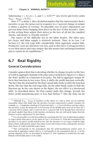
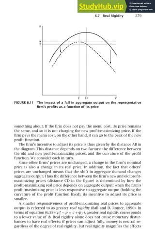
![280 Chapter 6 NOMINAL RIGIDITY
of nominal rigidity: the greater the degree of real rigidity, the larger the
range of prices for which nonadjustment of prices is an equilibrium.
The curvature of the profit function determines the cost of a given de-
parture of price from the profit-maximizing level. When profits are less sen-
sitive to departures from the optimum, the incentive for price adjustment
is smaller (for a given degree of real rigidity), and so the range of shocks
for which nonadjustment is an equilibrium is larger. Thus, in general terms,
what is needed for small costs of price adjustment to generate substantial
nominal rigidity is some combination of real rigidity and of insensitivity of
the profit function.
Seen in terms of real rigidity and insensitivity of the profit function, it is
easy to see why the incentive for price adjustment in our baseline calculation
is so large: there is immense “real flexibility” rather than real rigidity. Since
the profit-maximizing real price is [η/(η − 1)]Y1/ν
, its elasticity with respect
to output is 1/ν. If the elasticity of labor supply, ν, is small, the elasticity of
(Pi /P)∗ with respect to Y is large. A value of ν of 0.1, for example, implies
an elasticity of (Pi /P)∗ with respect to Y of 10.
An analogy may help to make clear how the combination of menu costs
with either real rigidity or insensitivity of the profit function (or both) can
lead to considerable nominal stickiness: monetary disturbances may have
real effects for the same reasons that the switch to daylight saving time
does.20
The resetting of clocks is a purely nominal change—it simply alters
the labels assigned to different times of day. But the change is associated
with changes in real schedules—that is, the times of various activities rel-
ative to the sun. And there is no doubt that the switch to daylight saving
time is the cause of the changes in real schedules.
If there were literally no cost to changing nominal schedules and commu-
nicating this information to others, daylight saving time would just cause
everyone to do this and would have no effect on real schedules. Thus for
daylight saving time to change real schedules, there must be some cost to
changing nominal schedules. These costs are analogous to the menu costs
of changing prices; and like the menu costs, they do not appear to be large.
The reason that these small costs cause the switch to have real effects is that
individuals and businesses are generally much more concerned about their
schedules relative to one another’s than about their schedules relative to
the sun. Thus, given that others do not change their scheduled hours, each
individual does not wish to incur the cost of changing his or hers. This is
analogous to the effects of real rigidity in the price-setting case. Finally, the
less concerned that individuals are about precisely what their schedules are,
the less willing they are to incur the cost of changing them; this is analogous
to the insensitivity of the profit function in the price-setting case.
20
This analogy is originally due to Friedman (1953, p. 173), in the context of exchange
rates.](https://image.slidesharecdn.com/advanced-macroeconomics-230806183016-1212def2/85/Advanced-Macroeconomics-302-320.jpg)


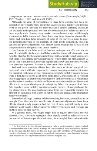
![284 Chapter 6 NOMINAL RIGIDITY
Sections 5.10 and 6.3, this view of the labor market has had limited empirical
success.
Second, imperfections in the labor market, such as those that are the
subject of Chapter 10, can cause workers to be off their labor supply curves
over at least part of the business cycle. The models presented there (in-
cluding more complicated models of search and matching frictions) break
the link between the elasticity of labor supply and the response of the
cost of labor to demand disturbances. Indeed, Chapter 10 presents several
models that imply relatively acyclical wages (or relatively acyclical costs of
labor to firms) despite inelastic labor supply. If imperfections like these
cause real wages to respond little to demand disturbances, they greatly
reduce firms’ incentive to vary their prices in response to these demand
shifts.24
A Second Quantitative Example
To see the potential importance of labor-market imperfections, consider the
following variation (from Ball and Romer, 1990) on our example of firms’
incentives to change prices in response to a monetary disturbance. Sup-
pose that for some reason firms pay wages above the market-clearing level,
and that the elasticity of the real wage with respect to aggregate output
is β:
W
P
= AY β
. (6.65)
Thus, as in Case 3 of Section 6.2, the cyclical behavior of the real wage is
determined by a “real-wage function” rather than by the elasticity of labor
supply.
With the remainder of the model as before, firm i’s profits are given by
(6.53) with the real wage equal to AY β
rather than Y1/ν
. It follows that
πi =
M
P
Pi
P
1−η
− A
M
P
1+β
Pi
P
−η
(6.66)
(compare [6.62]). The profit-maximizing real price is again η/(η − 1) times
the real wage; thus it is [η/(η − 1)]AY β
. It follows that equilibrium output
under flexible prices is [(η − 1)/(ηA)]1/β
. Assume that A and β are such that
24
In addition, the possibility of substantial real rigidities in the labor market suggests
that small barriers to nominal adjustment may cause nominal disturbances to have substan-
tial real effects through stickiness of nominal wages rather than of nominal prices. If wages
display substantial real rigidity, a demand-driven expansion leads only to small increases
in optimal real wages. As a result, just as small frictions in nominal price adjustment can
lead to substantial nominal price rigidity, so small frictions in nominal wage adjustment
can lead to substantial nominal wage rigidity.](https://image.slidesharecdn.com/advanced-macroeconomics-230806183016-1212def2/85/Advanced-Macroeconomics-306-320.jpg)
![6.7 Real Rigidity 285
labor supply at the flexible-price equilibrium exceeds the amount of labor
employed by firms.25
Now consider the representative firm’s incentive to change its price in the
face of a decline in aggregate demand, again assuming that other firms do
not change their prices. If the firm does not change its price, then Pi /P = 1,
and so (6.66) implies
πFIXED =
M
P
− A
M
P
1+β
. (6.67)
If the firm changes its price, it charges a real price of [η/(η − 1)]AY β
. Sub-
stituting this expression into (6.66) yields
πADJ =
M
P
η
η − 1
1−η
A1−η
M
P
β(1−η)
− A
M
P
1+β
η
η − 1
−η
A−η
M
P
−βη
= A1−η 1
η − 1
η
η − 1
−η
M
P
1+β−βη
.
(6.68)
If β, the parameter that governs the cyclical behavior of the real wage, is
small, the effect of this change in the model on the incentive for price adjust-
ment is dramatic. Suppose, for example, that β = 0.1, that η = 5 as before,
and that A = 0.806 (so that the flexible-price level of Y is 0.928, or about
95 percent of its level with ν = 0.1 and a clearing labor market). Substitut-
ing these parameter values into (6.67) and (6.68) implies that if the money
stock falls by 3 percent and firms do not adjust their prices, the represen-
tative firm’s gain from changing its price is approximately 0.0000168, or
about 0.0018 percent of the revenue it gets at the flexible-price equilibrium.
Even if M falls by 5 percent and β = 0.25 (and A is changed to 0.815,
so that the flexible-price level of Y continues to be 0.928), the incentive
for price adjustment is only 0.03 percent of the firm’s flexible-price
revenue.
This example shows how real rigidity and small barriers to nominal price
adjustment can produce a large amount of nominal rigidity. But the example
almost surely involves an unrealistic degree of real rigidity in the labor mar-
ket: the example assumes that the elasticity of the real wage with respect to
output is only 0.1, while the evidence discussed in Section 6.3 suggests that
the true elasticity is considerably higher. A more realistic account would
probably involve less real rigidity in the labor market, but would include
25
When prices are flexible, each firm sets its relative price to [η/(η − 1)](W/P). Thus the
real wage at the flexible-price equilibrium must be (η −1)/η, and so labor supply is [(η −1)/η]ν
.
Thus the condition that labor supply exceeds demand at the flexible-price equilibrium is
[(η − 1)/η]ν
[(η − 1)/(ηA)]1/β
.](https://image.slidesharecdn.com/advanced-macroeconomics-230806183016-1212def2/85/Advanced-Macroeconomics-307-320.jpg)

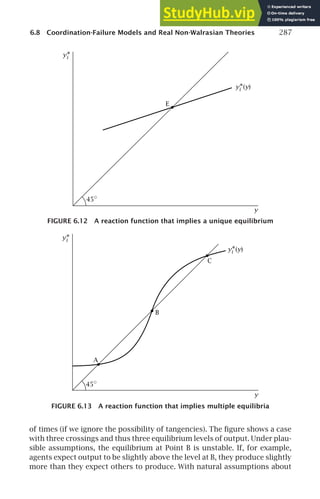
![6.8 Coordination-Failure Models and Real Non-Walrasian Theories 289
As noted above, there is a close connection between multiple equilibria
and real rigidity. The existence of multiple equilibria requires that over some
range, increases in aggregate output cause the representative producer to
want to lower its price and thus increase its output relative to others’. That
is, coordination failure requires that real rigidity be very strong over some
range. One implication of this observation is that since there are many po-
tential sources of real rigidity, there are many potential sources of coor-
dination failure. Thus there are many possible models that fit Cooper and
John’s general framework.
Empirical Application: Experimental Evidence on
Coordination-Failure Games
Coordination-failure models have more than one Nash equilibrium. Tradi-
tional game theory predicts that such economies will arrive at one of their
equilibria, but does not predict which one. Various theories of equilibrium
refinements make predictions about which equilibrium will be reached (as
do the extensions to heterogeneous information mentioned above). For ex-
ample, a common view is that Pareto-superior equilibria are focal, and that
economies where there is the potential for coordination failure therefore
attain the best possible equilibrium. There are other possibilities as well.
For example, it may be that each agent is unsure about what rule others
are using to choose among the possible outcomes, and that as a result such
economies do not reach any of their equilibria.
One approach to testing theories that has been pursued extensively in re-
cent years, especially in game theory, is the use of experiments. Experiments
have the advantage that they allow researchers to control the economic en-
vironment precisely. They have the disadvantages, however, that they are
often not feasible and that behavior may be different in the laboratory than
in similar situations in practice.
An example of this approach in the context of coordination-failure mod-
els is the test of the game proposed by Bryant (1983) that is conducted by
Van Huyck, Battalio, and Beil (1990). In Bryant’s game, each of N agents
chooses an effort level over the range [0,e]. The payoff to agent i is
Ui = αmin[e1,e2, . . . ,eN] − βei , α β 0. (6.69)
The best Nash equilibrium is for every agent to choose the maximum effort
level, e; this gives each agent a payoff of (α − β)e. But any common effort
level in [0,e] is also a Nash equilibrium: if every agent other than agent i
sets his or her effort to some level ê, i also wants to choose effort of ê. Since
each agent’s payoff is increasing in the common effort level, Bryant’s game
is a coordination-failure model with a continuum of equilibria.
Van Huyck, Battalio, and Beil consider a version of Bryant’s game with
effort restricted to the integers 1 through 7, α = $0.20, β = $0.10, and N](https://image.slidesharecdn.com/advanced-macroeconomics-230806183016-1212def2/85/Advanced-Macroeconomics-311-320.jpg)
![294 Chapter 6 NOMINAL RIGIDITY
for good i is given by
yi = y + zi − η(pi − p), η 0, (6.76)
where zi is the good-specific demand shock. We assume that the aggregate
demand equation (6.41), y = m − p, holds as before. Thus (6.76) becomes
yi = (m − p) + zi − η(pi − p). (6.77)
Note that aside from the presence of the zi term, this is the same as the
demand curve in the model in Section 6.5, equation (6.48).
With heterogeneous demands arising from taste shocks, the price index
corresponding to individuals’ utility function takes a somewhat more com-
plicated form than the previous price index, (6.47). For simplicity, we there-
fore define the log price index, p, to be just the average log price:
p = pi . (6.78)
Similarly, we define
y = yi . (6.79)
Using the more theoretically appropriate definitions of p and y would have
no effects on the messages of the model.
The model’s key assumption is that the producer cannot observe zi and
m. Instead, it can only observe the price of its good, pi . We can write pi as
pi = p + (pi − p)
≡ p + ri ,
(6.80)
where ri ≡ pi − p is the relative price of good i. Thus, in logs, the variable
that the producer observes—the price of its good—equals the sum of the
aggregate price level and the good’s relative price.
The producer would like to base its production decision on ri alone (see
[6.75]). The producer does not observe ri , but must estimate it given the
observation of pi .28
At this point, Lucas makes two simplifying assumptions.
First, he assumes that the producer finds the expectation of ri given pi , and
then produces as much as it would if this estimate were certain. Thus (6.75)
becomes
yi =
1
γ − 1
E [ri |pi ]. (6.81)
28
Recall that the firm is owned by a single household. If the household knew others’
prices as a result of making purchases, it could deduce p, and hence ri . This can be ruled out
in several ways. One approach is to assume that the household consists of two individuals, a
“producer” and a “shopper,” and that communication between them is limited. In his original
model, Lucas avoids the problem by assuming an overlapping-generations structure where
individuals produce in the first period of their lives and make purchases in the second.](https://image.slidesharecdn.com/advanced-macroeconomics-230806183016-1212def2/85/Advanced-Macroeconomics-316-320.jpg)
![6.9 The Lucas Imperfect-Information Model 295
As Problem 6.14 shows, this certainty-equivalence behavior is not identical
to maximizing expected utility: in general, the utility-maximizing choice of
yi depends not just on the household’s point estimate of ri , but also on
its uncertainty. Like the assumption that p = Pi , however, the assumption
that households use certainty equivalence simplifies the analysis and has
no effect on the central messages of the model.
Second, Lucas assumes that the monetary shock (m) and the shocks to
the demands for the individual goods (the zi ’s) are normally distributed.
m has a mean of E [m] and a variance of Vm. The zi ’s have a mean of 0 and a
variance of Vz, and are independent of m. We will see that these assumptions
imply that p and ri are normal and independent.
Finally, one assumption of the model is so commonplace today that we
passed over it without comment: in assuming that the producer chooses
how much to produce based on the mathematical expectation of ri , E[ri |pi ],
we implicitly assumed that the producer finds expectations rationally. That
is, the expectation of ri is assumed to be the true expectation of ri given pi
and given the actual joint distribution of the two variables. Today, this as-
sumption of rational expectations seems no more peculiar than the assump-
tion that individuals maximize utility. But when Lucas introduced rational
expectations into macroeconomics, it was highly controversial. As we will
see, it is one source—but by no means the only one—of the strong implica-
tions of his model.
The Lucas Supply Curve
We will solve the model by tentatively assuming that p and ri are normal
and independent, and then verifying that the equilibrium does indeed have
this property.
Since pi equals p + ri , the assumption that p and ri are normal and in-
dependent implies that pi is also normal; its mean is the sum of the means
of p and ri , and its variance is the sum of their variances. An important re-
sult in statistics is that when two variables are jointly normally distributed
(as with ri and pi here), the expectation of one is a linear function of the
observation of the other. In this particular case, where pi equals ri plus an
independent variable, the expectation takes the specific form
E[ri |pi ] = E[ri ] +
Vr
Vr + Vp
(pi − E[pi ])
(6.82)
=
Vr
Vr + Vp
(pi − E[pi ]),
where Vr and Vp are the variances of p and ri , and where the second line
uses the fact that the symmetry of the model implies that the mean of each
relative price is zero.](https://image.slidesharecdn.com/advanced-macroeconomics-230806183016-1212def2/85/Advanced-Macroeconomics-317-320.jpg)
![296 Chapter 6 NOMINAL RIGIDITY
Equation (6.82) is intuitive. First, it implies that if pi equals its mean,
the expectation of ri equals its mean (which is 0). Second, it states that the
expectation of ri exceeds its mean if pi exceeds its mean, and is less than
its mean if pi is less than its mean. Third, it tells us that the fraction of the
departure of pi from its mean that is estimated to be due to the departure of
ri from its mean is Vr/(Vr + Vp); this is the fraction of the overall variance
of pi (which is Vr + Vp) that is due to the variance of ri (which is Vr). If,
for example, Vp is 0, all the variation in pi is due to ri , and so E [ri |pi ] is
pi − E [p]. If Vr and Vp are equal, half of the variance in pi is due to ri , and
so E [ri |pi ] = (pi − E [p])/2. And so on.
This conditional-expectations problem is referred to as signal extraction.
The variable that the individual observes, pi , equals the signal, ri , plus noise,
p. Equation (6.82) shows how the individual can best extract an estimate of
the signal from the observation of pi . The ratio of Vr to Vp is referred to as
the signal-to-noise ratio.
Recall that the producer’s output is given by yi = [1/(γ −1)]E[ri |pi ] (equa-
tion [6.81]). Substituting (6.82) into this expression yields
yi =
1
γ − 1
Vr
Vr + Vp
(pi − E [p])
≡ b(pi − E [p]).
(6.83)
Averaging (6.83) across producers (and using the definitions of y and p)
gives us an expression for overall output:
y = b(p− E [p]). (6.84)
Equation (6.84) is the Lucas supply curve. It states that the departure of
output from its normal level (which is zero in the model) is an increasing
function of the surprise in the price level.
The Lucas supply curve is essentially the same as the expectations-
augmented Phillips curve of Section 6.4 with core inflation replaced by ex-
pected inflation (see equation [6.24]). Both state that if we neglect distur-
bances to supply, output is above normal only to the extent that inflation
(and hence the price level) is greater than expected. Thus the Lucas model
provides microeconomic foundations for this view of aggregate supply.
Equilibrium
Combining the Lucas supply curve with the aggregate demand equation,
y = m −p, and solving for p and y yields
p =
1
1 + b
m +
b
1 + b
E [p], (6.85)
y =
b
1 + b
m −
b
1 + b
E [p]. (6.86)](https://image.slidesharecdn.com/advanced-macroeconomics-230806183016-1212def2/85/Advanced-Macroeconomics-318-320.jpg)
![6.9 The Lucas Imperfect-Information Model 297
We can use (6.85) to find E [p]. Ex post, after m is determined, the two sides
of (6.85) are equal. Thus it must be that ex ante, before m is determined,
the expectations of the two sides are equal. Taking the expectations of both
sides of (6.85), we obtain
E [p] =
1
1 + b
E [m] +
b
1 + b
E [p]. (6.87)
Solving for E [p] yields
E [p] = E [m]. (6.88)
Using (6.88) and the fact that m = E [m] + (m − E [m]), we can rewrite
(6.85) and (6.86) as
p = E [m] +
1
1 + b
(m − E [m]), (6.89)
y =
b
1 + b
(m − E [m]). (6.90)
Equations (6.89) and (6.90) show the key implications of the model: the
component of aggregate demand that is observed, E [m], affects only prices,
but the component that is not observed, m − E [m], has real effects. Con-
sider, for concreteness, an unobserved increase in m—that is, a higher real-
ization of m given its distribution. This increase in the money supply raises
aggregate demand, and thus produces an outward shift in the demand curve
for each good. Since the increase is not observed, each supplier’s best guess
is that some portion of the rise in the demand for his or her product reflects
a relative price shock. Thus producers increase their output.
The effects of an observed increase in m are very different. Specifically,
consider the effects of an upward shift in the entire distribution of m, with
the realization of m − E [m] held fixed. In this case, each supplier attributes
the rise in the demand for his or her product to money, and thus does not
change his or her output. Of course, the taste shocks cause variations in
relative prices and in output across goods (just as they do in the case of an
unobserved shock), but on average real output does not rise. Thus observed
changes in aggregate demand affect only prices.
To complete the model, we must express b in terms of underlying pa-
rameters rather than in terms of the variances of p and ri . Recall that b =
[1/(γ −1)][Vr/(Vr +Vp)] (see [6.83]). Equation (6.89) implies Vp = Vm/(1 +b)2
.
The demand curve, (6.76), and the supply curve, (6.84), can be used to find
Vr, the variance of pi − p. Specifically, we can substitute y = b(p − E [p])
into (6.76) to obtain yi = b(p − E [p]) + zi − η(pi − p), and we can rewrite
(6.83) as yi = b(pi − p) + b(p − E [p]). Solving these two equations for pi − p
then yields pi − p = zi /(η+ b). Thus Vr = Vz/(η+ b)2
.](https://image.slidesharecdn.com/advanced-macroeconomics-230806183016-1212def2/85/Advanced-Macroeconomics-319-320.jpg)
![298 Chapter 6 NOMINAL RIGIDITY
Substituting the expressions for Vp and Vr into the definition of b (see
[6.83]) yields
b =
1
γ − 1
⎡
⎣
Vz
Vz +
(η + b)2
(1 + b)2
Vm
⎤
⎦. (6.91)
Equation (6.91) implicitly defines b in terms of Vz, Vm, and γ , and thus com-
pletes the model. It is straightforward to show that b is increasing in Vz and
decreasing in Vm. In the special case of η = 1, we can obtain a closed-form
expression for b:
b =
1
γ − 1
Vz
Vz + Vm
. (6.92)
Finally, note that the results that p = E [m] + [1/(1 + b)](m − E [m]) and
ri = zi /(η + b) imply that p and ri are linear functions of m and zi . Since
m and zi are independent, p and ri are independent. And since linear func-
tions of normal variables are normal, p and ri are normal. This confirms the
assumptions made above about these variables.
The Phillips Curve and the Lucas Critique
Lucas’s model implies that unexpectedly high realizations of aggregate de-
mand lead to both higher output and higher-than-expected prices. As a re-
sult, for reasonable specifications of the behavior of aggregate demand, the
model implies a positive association between output and inflation. Suppose,
for example, that m is a random walk with drift:
mt = mt −1 + c + ut, (6.93)
where u is white noise. This specification implies that the expectation of
mt is mt −1 + c and that the unobserved component of mt is ut. Thus, from
(6.89) and (6.90),
pt = mt −1 + c +
1
1 + b
ut, (6.94)
yt =
b
1 + b
ut. (6.95)
Equation (6.94) implies that pt −1 = mt −2 + c + [ut −1/(1 + b)]. The rate of
inflation (measured as the change in the log of the price level) is thus
πt = (mt −1 − mt −2) +
1
1 + b
ut −
1
1 + b
ut −1
= c +
b
1 + b
ut −1 +
1
1 + b
ut.
(6.96)](https://image.slidesharecdn.com/advanced-macroeconomics-230806183016-1212def2/85/Advanced-Macroeconomics-320-320.jpg)
![6.9 The Lucas Imperfect-Information Model 299
Note that ut appears in both (6.95) and (6.96) with a positive sign, and
that ut and ut −1 are uncorrelated. These facts imply that output and inflation
are positively correlated. Intuitively, high unexpected money growth leads,
through the Lucas supply curve, to increases in both prices and output.
The model therefore implies a positive relationship between output and
inflation—a Phillips curve.
Crucially, however, although there is a statistical output-inflation rela-
tionship in the model, there is no exploitable tradeoff between output and
inflation. Suppose policymakers decide to raise average money growth (for
example, by raising c in equation [6.93]). If the change is not publicly known,
there is an interval when unobserved money growth is typically positive, and
output is therefore usually above normal. Once individuals determine that
the change has occurred, however, unobserved money growth is again on
average zero, and so average real output is unchanged. And if the increase
in average money growth is known, expected money growth jumps imme-
diately and there is not even a brief interval of high output. The idea that
the statistical relationship between output and inflation may change if pol-
icymakers attempt to take advantage of it is not just a theoretical curiosity:
as we saw in Section 6.4, when average inflation rose in the late 1960s and
early 1970s, the traditional output-inflation relationship collapsed.
The central idea underlying this analysis is of wider relevance. Expec-
tations are likely to be important to many relationships among aggregate
variables, and changes in policy are likely to affect those expectations. As a
result, shifts in policy can change aggregate relationships. In short, if poli-
cymakers attempt to take advantage of statistical relationships, effects op-
erating through expectations may cause the relationships to break down.
This is the famous Lucas critique (Lucas, 1976).
Stabilization Policy
The result that only unobserved aggregate demand shocks have real effects
has a strong implication: monetary policy can stabilize output only if policy-
makers have information that is not available to private agents. Any portion
of policy that is a response to publicly available information—such as the
unemployment rate or the index of leading indicators—is irrelevant to the
real economy (Sargent and Wallace, 1975; Barro, 1976).
To see this, let aggregate demand, m, equal m∗ + v, where m∗ is a pol-
icy variable and v a disturbance outside the government’s control. If the
government does not pursue activist policy but simply keeps m∗ constant
(or growing at a steady rate), the unobserved shock to aggregate demand
in some period is the realization of v less the expectation of v given the
information available to private agents. If m∗ is instead a function of public
information, individuals can deduce m∗, and so the situation is unchanged.
Thus systematic policy rules cannot stabilize output.](https://image.slidesharecdn.com/advanced-macroeconomics-230806183016-1212def2/85/Advanced-Macroeconomics-321-320.jpg)


![6.10 International Evidence on the Output-Inflation Tradeoff 303
the determinants of the strength of those effects. This is the approach pio-
neered by Lucas (1973).
The Variability of Demand
In the Lucas model, suppliers’ responses to changes in prices are determined
by the relative importance of aggregate and idiosyncratic shocks. If aggre-
gate shocks are large, for example, suppliers attribute most of the changes
in the prices of their goods to changes in the price level, and so they al-
ter their production relatively little in response to variations in prices (see
[6.83]). The Lucas model therefore predicts that the real effect of a given
aggregate demand shock is smaller in an economy where the variance of
those shocks is larger.
To test this prediction, one must find a measure of aggregate demand
shocks. Lucas (1973) uses the change in the log of nominal GDP. For this to
be precisely correct, two conditions must be satisfied. First, the aggregate
demand curve must be unit-elastic; that is, nominal GDP must be deter-
mined entirely by aggregate demand, so that changes in aggregate supply
affect P and Y but not their product. Second, the change in log nominal GDP
must not be predictable or observable. That is, letting x denote log nominal
GDP, x must take the form a + ut, where ut is white noise. With this pro-
cess, the change in log nominal GDP (relative to its average change) is also
the unobserved change. Although these conditions are surely not satisfied
exactly, they may be accurate enough to be reasonable approximations.
Under these assumptions, the real effects of an aggregate demand shock
in a given country can be estimated by regressing log real GDP (or the change
in log real GDP) on the change in log nominal GDP and control variables. The
specification Lucas employs is
yt = c + γt + τxt + λyt −1, (6.97)
where y is log real GDP, t is time, and x is the change in log nominal GDP.
Lucas estimates (6.97) separately for various countries. He then asks
whether the estimated τ’s—the estimates of the responsiveness of output to
aggregate demand movements—are related to the average size of countries’
aggregate demand shocks. A simple way to do this is to estimate
τi = α + βσx,i , (6.98)
where τi is the estimate of the real impact of an aggregate demand shift
obtained by estimating (6.97) for country i and σx,i is the standard devia-
tion of the change in log nominal GDP in country i. Lucas’s theory predicts
that nominal shocks have smaller real effects in settings where aggregate
demand is more volatile, and thus that β is negative.
Lucas employs a relatively small sample. His test has been extended to
much larger samples, with various modifications in specification, in several
studies. Figure 6.15, from Ball, Mankiw, and D. Romer (1988), is typical of](https://image.slidesharecdn.com/advanced-macroeconomics-230806183016-1212def2/85/Advanced-Macroeconomics-325-320.jpg)
![6.10 International Evidence on the Output-Inflation Tradeoff 305
−0.2
−0.3
−0.1
0
0.1
0.2
0.3
0.4
0.5
0.6
0.7
0.9
0.8
Mean inflation
0.6
0.2 0.4
τ
FIGURE 6.16 The output-inflation tradeoff and average inflation (from Ball,
Mankiw, and Romer, 1988)
a quadratic term included to account for the nonlinearity apparent in the
figure) is
τi = 0.600
(0.079)
− 4.835
(1.074)
πi + 7.118
(2.088)
π2
i ,
R
2
= 0.388, s.e.e. = 0.215,
(6.100)
where πi is average inflation in country i and the numbers in parenthe-
ses are standard errors. The point estimates imply that ∂τ/∂π = −4.835 +
2(7.118)π, which is negative for π 4.835/[2(7.118)] ≃ 34%. Thus there is a
statistically significant negative relationship between average inflation and
the estimated real impact of aggregate demand movements.
Countries with higher average inflation generally have more variable ag-
gregate demand. Thus it is possible that the results in (6.100) arise not
because π directly affects τ, but because it is correlated with the standard
deviation of nominal GNP growth (σx), which does directly affect τ. Alter-
natively, it is possible that Lucas’s results arise from the fact that σx and π
are correlated.
The appropriate way to test between these two views is to run a “horse-
race” regression that includes both variables. Again quadratic terms are
included to allow for nonlinearities. The results are
τi = 0.589
(0.086)
− 5.729
(1.973)
πi + 8.406
(3.849)
π2
i + 1.241
(2.467)
σx − 2.380
(7.062)
σ2
x ,
(6.101)
R
2
= 0.359, s.e.e. = 0.219.](https://image.slidesharecdn.com/advanced-macroeconomics-230806183016-1212def2/85/Advanced-Macroeconomics-327-320.jpg)
![306 Chapter 6 NOMINAL RIGIDITY
The coefficients on the average inflation variables are essentially the same
as in the previous regression, and they remain statistically significant. The
variability terms, in contrast, play little role. The null hypothesis that the co-
efficients on both σx and σ2
x are zero cannot be rejected at any reasonable
confidence level, and the point estimates imply that reasonable changes in
σx have quantitatively small effect on τ. For example, a change in σx from
0.05 to 0.10 changes τ by only 0.04. Thus the results appear to favor the
menu-cost view over the Lucas model.31
Kiley (2000) extends the analysis to the persistence of output movements.
He first notes that menu-cost models imply that departures of output from
normal are less persistent when average inflation is higher. The intuition
is again that higher average inflation increases the frequency of price ad-
justment, and therefore causes the economy to return to its flexible-price
equilibrium more rapidly after a shock. He finds that the data support this
implication as well.
Problems
6.1. Describe how, if at all, each of the following developments affect the curves in
Figure 6.1:
(a) The coefficient of relative risk aversion, θ, rises.
(b) The curvature of ⌫(•), ν falls.
(c) We modify the utility function, (6.2), to be
βt
[U(Ct) + B⌫(Mt/Pt) −
V(Lt)], B 0, and B falls.
6.2. The Baumol-Tobin model. (Baumol, 1952; Tobin, 1956.) Consider a consumer
with a steady flow of real purchases of amount αY, 0 α ≤ 1, that are made
with money. The consumer chooses how often to convert bonds, which pay a
constant interest rate of i, into money, which pays no interest. If the consumer
chooses an interval of τ, his or her money holdings decline linearly from αYPτ
after each conversion to zero at the moment of the next conversion (here P is
the price level, which is assumed constant). Each conversion has a fixed real
cost of C. The consumer’s problem is to choose τ to minimize the average cost
per unit time of conversions and foregone interest.
(a) Find the optimal value of τ.
(b) What are the consumer’s average real money holdings? Are they decreasing
in i and increasing in Y ? What is the elasticity of average money holdings
with respect to i ? With respect to Y ?
6.3. The multiplier-accelerator. (Samuelson, 1939.) Consider the following model
of income determination. (1) Consumption depends on the previous period’s
31
The lack of a discernable link between σx and τ, however, is a puzzle not only for the
Lucas model but also for models based on barriers to price adjustment: an increase in the
variability of shocks should make firms change their prices more often, and should therefore
reduce the real impact of a change in aggregate demand.](https://image.slidesharecdn.com/advanced-macroeconomics-230806183016-1212def2/85/Advanced-Macroeconomics-328-320.jpg)
![308 Chapter 6 NOMINAL RIGIDITY
(c) Suppose increases in money also affect expected inflation. Specifically,
assume that dπe
/dm is exogenous, with dπe
/dm 0. Continue to as-
sume 0 dp/dm 1. Find an expression for dr/dm. Does an increase
in the money supply lower the real interest rate? Does achieving a given
change in r require a change in m smaller, larger, or the same size as in
part (b)?
(d) Suppose there is complete and instantaneous price adjustment: dp/dm =
1, dπe
/dm = 0. Find an expression for dr/dm. Does an increase in the
money supply lower the real interest rate?
6.7. The liquidity trap. Consider the following model. The dynamics of inflation
are given by the continuous-time version of (6.22)–(6.23): π̇(t) = λ[y(t)−y (t)],
λ 0. The IS curve takes the traditional form, y(t) = −[i(t)−π(t)]/θ, θ 0. The
central bank sets the interest rate according to (6.26), but subject to the con-
straint that the nominal interest rate cannot be negative: i(t) = max[0,π(t) +
r(y(t) − y(t),π(t))]. For simplicity, normalize y(t) = 0 for all t.
(a) Sketch the aggregate demand curve for this model—that is, the set of
points in (y,π) space that satisfy the IS equation and the rule above for
the interest rate.
(b) Let (ỹ,π̃) denote the point on the aggregate demand curve where π +
r(y,π) = 0. Sketch the paths of y and π over time if:
(i) ỹ 0, π(0) π̃, and y (0) 0.
(ii) ỹ 0 and π(0) π̃.
(iii) ỹ 0, π(0) π̃, and y (0) 0.32
6.8. Consider the model in equations (6.27)–(6.30). Suppose, however, that there
are shocks to the MP equation but not to the IS equation. Thus rt = byt +
uMP
t , uMP
t = ρMP uMP
t + eMP
t (where −1 ρMP 1 and eMP
is white noise), and
yt = Et yt+1 − 1
θ
rt. Find the expression analogous to (6.35).
6.9. (a) Consider the model in equations (6.27)–(6.30). Solve the model using the
method of undetermined coefficients. That is, conjecture that the solution
takes the form yt = AuIS
t , and find the value that A must take for the
equations of the model to hold. (Hint: The fact that yt = AuIS
t for all t
implies Et yt+1 = A EtuIS
t+1.)
(b) Now modify the MP equation to be rt = byt + cπt. Conjecture that the
solution takes the form yt = AuIS
t + Bπt−1, πt = CuIS
t + Dπt−1. Find (but do
not solve) four equations that A, B, C, and D must satisfy for the equations
of the model to hold.
6.10. Multiple equilibria with menu costs. (Ball and D. Romer, 1991.) Consider an
economy consisting of many imperfectly competitive firms. The profits that
a firm loses relative to what it obtains with pi = p∗ are K(pi − p∗)2
, K 0. As
usual, p∗ = p +φy and y = m − p. Each firm faces a fixed cost Z of changing
its nominal price.
32
See Section 11.6 for more on the zero lower bound on the nominal interest rate.](https://image.slidesharecdn.com/advanced-macroeconomics-230806183016-1212def2/85/Advanced-Macroeconomics-330-320.jpg)
![Problems 309
Initially m is 0 and the economy is at its flexible-price equilibrium, which
is y = 0 and p = m= 0. Now suppose m changes to m′
.
(a) Suppose that fraction f of firms change their prices. Since the firms that
change their prices charge p∗ and the firms that do not charge 0, this
implies p = f p∗. Use this fact to find p, y, and p∗ as functions of m′
and f .
(b) Plot a firm’s incentive to adjust its price, K(0− p∗)2
= Kp∗2
, as a function
of f . Be sure to distinguish the cases φ 1 and φ 1.
(c) A firm adjusts its price if the benefit exceeds Z, does not adjust if the
benefit is less than Z, and is indifferent if the benefit is exactly Z. Given
this, can there be a situation where both adjustment by all firms and
adjustment by no firms are equilibria? Can there be a situation where
neither adjustment by all firms nor adjustment by no firms is an
equilibrium?
6.11. Consider an economy consisting of many imperfectly competitive, price-
setting firms. The profits of the representative firm, firm i, depend on ag-
gregate output, y, and the firm’s real price, ri : πi = π(y,ri ), where π22 0
(subscripts denote partial derivatives). Let r∗(y) denote the profit-maximizing
price as a function of y; note that r∗(y) is characterized by π2(y,r∗(y)) = 0.
Assume that output is at some level y0, and that firm i’s real price is r∗(y0).
Now suppose there is a change in the money supply, and suppose that other
firms do not change their prices and that aggregate output therefore changes
to some new level, y1.
(a) Explain why firm i’s incentive to adjust its price is given by G = π(y1,
r∗(y1)) − π(y1,r∗(y0)).
(b) Use a second-order Taylor approximation of this expression in y1 around
y1 = y0 to show that G ≃ −π22(y0,r∗(y0))[r∗′
(y0)]2
(y1 − y0)2
/2.
(c) What component of this expression corresponds to the degree of real
rigidity? What component corresponds to the degree of insensitivity of
the profit function?
6.12. Indexation. (This problem follows Ball, 1988.) Suppose production at firm
i is given by Yi = SLα
i , where S is a supply shock and 0 α ≤ 1. Thus
in logs, yi = s + αℓi . Prices are flexible; thus (setting the constant term to
0 for simplicity), pi = wi + (1 − α)ℓi − s. Aggregating the output and price
equations yields y = s + αℓ and p = w + (1 − α)ℓ − s. Wages are partially
indexed to prices: w = θp, where 0 ≤ θ ≤ 1. Finally, aggregate demand is
given by y = m − p. s and m are independent, mean-zero random variables
with variances Vs and Vm.
(a) What are p, y, ℓ, and w as functions of m and s and the parameters α and
θ? How does indexation affect the response of employment to monetary
shocks? How does it affect the response to supply shocks?
(b) What value of θ minimizes the variance of employment?
(c) Suppose the demand for a single firm’s output is yi = y − η(pi − p).
Suppose all firms other than firm i index their wages by w = θp as before,
but that firm i indexes its wage by wi = θi p. Firm i continues to set its](https://image.slidesharecdn.com/advanced-macroeconomics-230806183016-1212def2/85/Advanced-Macroeconomics-331-320.jpg)
![310 Chapter 6 NOMINAL RIGIDITY
price as pi = wi + (1 − α)ℓi − s. The production function and the pricing
equation then imply that yi = y − φ(wi − w), where φ≡ αη/[α+ (1 − α)η].
(i) What is employment at firm i, ℓi , as a function of m, s, α, η, θ, and θi ?
(ii) What value of θi minimizes the variance of ℓi ?
(iii) Find the Nash equilibrium value of θ. That is, find the value of θsuch
that if aggregate indexation is given by θ, the representative firm
minimizes the variance of ℓi by setting θi = θ. Compare this value
with the value found in part (b).
6.13. Thick-market effects and coordination failure. (This follows Diamond,
1982.)33
Consider an island consisting of N people and many palm trees.
Each person is in one of two states, not carrying a coconut and looking for
palm trees (state P) or carrying a coconut and looking for other people with
coconuts (state C ). If a person without a coconut finds a palm tree, he or she
can climb the tree and pick a coconut; this has a cost (in utility units) of c.
If a person with a coconut meets another person with a coconut, they trade
and eat each other’s coconuts; this yields u units of utility for each of them.
(People cannot eat coconuts that they have picked themselves.)
A person looking for coconuts finds palm trees at rate b per unit time.
A person carrying a coconut finds trading partners at rate aL per unit time,
where L is the total number of people carrying coconuts. a and b are
exogenous.
Individuals’ discount rate is r. Focus on steady states; that is, assume that
L is constant.
(a) Explain why, if everyone in state P climbs a palm tree whenever he or she
finds one, then rVP = b(VC − VP − c), where VP and VC are the values of
being in the two states.
(b) Find the analogous expression for VC.
(c) Solve for VC − VP , VC, and VP in terms of r, b, c, u, a, and L.
(d) What is L, still assuming that anyone in state P climbs a palm tree when-
ever he or she finds one? Assume for simplicity that aN = 2b.
(e) For what values of c is it a steady-state equilibrium for anyone in state
P to climb a palm tree whenever he or she finds one? (Continue to assume
aN = 2b.)
(f) For what values of c is it a steady-state equilibrium for no one who finds
a tree to climb it? Are there values of c for which there is more than one
steady-state equilibrium? If there are multiple equilibria, does one involve
higher welfare than the other? Explain intuitively.
6.14. Consider the problem facing an individual in the Lucas model when Pi /P is
unknown. The individual chooses Li to maximize the expectation of Ui ; Ui
continues to be given by equation (6.72).
33
The solution to this problem requires dynamic programming (see Section 10.4).](https://image.slidesharecdn.com/advanced-macroeconomics-230806183016-1212def2/85/Advanced-Macroeconomics-332-320.jpg)
![Problems 311
(a) Find the first-order condition for Yi , and rearrange it to obtain an expres-
sion for Yi in terms of E [Pi /P]. Take logs of this expression to obtain an
expression for yi .
(b) How does the amount of labor the individual supplies if he or she fol-
lows the certainty-equivalence rule in (6.81) compare with the optimal
amount derived in part (a)? (Hint: How does E [ln(Pi /P)] compare with
ln(E [Pi /P])?)
(c) Suppose that (as in the Lucas model) ln(Pi /P) = E [ln(Pi /P) |Pi ]+ui , where
ui is normal with a mean of 0 and a variance that is independent of Pi .
Show that this implies that ln{E [(Pi /P) |Pi ]} = E [ln(Pi /P) |Pi ] + C, where
C is a constant whose value is independent of Pi . (Hint: Note that Pi /P =
exp{E [ln(Pi /P) |Pi ]}exp(ui ), and show that this implies that the yi that
maximizes expected utility differs from the certainty-equivalence rule in
(6.81) only by a constant.)
6.15. Observational equivalence. (Sargent, 1976.) Suppose that the money supply
is determined by mt = c ′
zt −1 + et, where c and z are vectors and et is an i.i.d.
disturbance uncorrelated with zt −1. et is unpredictable and unobservable.
Thus the expected component of mt is c ′
zt −1, and the unexpected component
is et. In setting the money supply, the Federal Reserve responds only to vari-
ables that matter for real activity; that is, the variables in z directly affect y.
Now consider the following two models: (i) Only unexpected money mat-
ters, so yt = a′
zt −1+bet +vt; (ii) all money matters, so yt = α′
zt −1+βmt +νt. In
each specification, the disturbance is i.i.d. and uncorrelated with zt −1 and et.
(a) Is it possible to distinguish between these two theories? That is, given a
candidate set of parameter values under, say, model (i), are there param-
eter values under model (ii) that have the same predictions? Explain.
(b) Suppose that the Federal Reserve also responds to some variables that
do not directly affect output; that is, suppose mt = c ′
zt −1 + γ ′
wt −1 + et
and that models (i) and (ii) are as before (with their distubances now
uncorrelated with wt −1 as well as with zt −1 and et). In this case, is it pos-
sible to distinguish between the two theories? Explain.
6.16. Consider an economy consisting of some firms with flexible prices and some
with rigid prices. Let pf
denote the price set by a representative flexible-price
firm and pr
the price set by a representative rigid-price firm. Flexible-price
firms set their prices after m is known; rigid-price firms set their prices be-
fore m is known. Thus flexible-price firms set pf
= p∗
i = (1 − φ)p + φm,
and rigid-price firms set pr
= E p∗
i = (1 − φ)E p + φEm, where E denotes the
expectation of a variable as of when the rigid-price firms set their prices.
Assume that fraction q of firms have rigid prices, so that p = qpr
+ (1−q)pf
.
(a) Find pf
in terms of pr
, m, and the parameters of the model (φ and q).
(b) Find pr
in terms of Em and the parameters of the model.
(c) (i) Do anticipated changes in m (that is, changes that are expected as of
when rigid-price firms set their prices) affect y? Why or why not?
(ii) Do unanticipated changes in m affect y? Why or why not?](https://image.slidesharecdn.com/advanced-macroeconomics-230806183016-1212def2/85/Advanced-Macroeconomics-333-320.jpg)


![7.1 Building Blocks of Dynamic New Keynesian Models 315
many reasons—involving uncertainty, information and renegotiation costs,
incentives, and so on—that prices and wages may not adjust freely to equate
supply and demand, or that firms may not change their prices and wages
completely and immediately in response to shocks. But simply introducing
some departure from perfect markets is not enough to imply that nomi-
nal disturbances matter. All the models of unemployment in Chapter 10,
for example, are real models. If one appends a monetary sector to those
models without any further complications, the classical dichotomy contin-
ues to hold: monetary disturbances cause all nominal prices and wages to
change, leaving the real equilibrium (with whatever non-Walrasian features
it involves) unchanged. Any microeconomic basis for failure of the classical
dichotomy requires some kind of nominal imperfection.
7.1 Building Blocks of Dynamic New
Keynesian Models
Overview
We will analyze the various models of dynamic price adjustment in a com-
mon framework. The framework draws heavily on the model of exogenous
nominal rigidity in Section 6.1 and the model of imperfect competition in
Section 6.5.
Time is discrete. Each period, imperfectly competitive firms produce out-
put using labor as their only input. As in Section 6.5, the production func-
tion is one-for-one; thus aggregate output and aggregate labor input are
equal. The model omits the government and international trade; thus, as in
the models of Chapter 6, aggregate consumption and aggregate output are
equal.
For simplicity, for the most part we will neglect uncertainty. Households
maximize utility, taking the paths of the real wage and the real interest rate
as given. Firms, which are owned by the households, maximize the present
discounted value of their profits, subject to constraints on their price-setting
(which vary across the models we will consider). Finally, a central bank de-
termines the path of the real interest rate through its conduct of monetary
policy.
Households
There is a fixed number of infinitely lived households that obtain utility from
consumption and disutility from working. The representative household’s
objective function is
∞
t =0
βt
[U(Ct) − V (Lt)], 0 β 1. (7.1)](https://image.slidesharecdn.com/advanced-macroeconomics-230806183016-1212def2/85/Advanced-Macroeconomics-337-320.jpg)
![316 Chapter 7 DSGE MODELS OF FLUCTUATIONS
As in Section 6.5, C is a consumption index that is a constant-elasticity-of-
substitution combination of the household’s consumption of the individual
goods, with elasticity of substitution η 1. We make our usual assumptions
about the functional forms of U(•) and V(•):1
U(Ct) =
C1−θ
t
1 − θ
, θ 0, (7.2)
V(Lt) =
B
γ
L
γ
t , B 0, γ 1. (7.3)
Let W denote the nominal wage and P denote the price level. Formally, P is
the price index corresponding to the consumption index, as in Section 6.5.
Throughout this chapter, however, we use the approximation we used in
the Lucas model in Section 6.9 that the log of the price index, which we will
denote p, is simply the average of firms’ log prices.
An increase in labor supply in period t of amount dL increases the house-
hold’s real income by (Wt/Pt) dL. The first-order condition for labor supply
in period t is therefore
V ′
(Lt) = U ′
(Ct)
Wt
Pt
. (7.4)
Because the production function is one-for-one and the only possible use
of output is for consumption, in equilibrium Ct and Lt must both equal Yt.
Combining this fact with (7.4) tells us what the real wage must be given the
level of output:
Wt
Pt
=
V ′
(Yt)
U ′
(Yt)
. (7.5)
Substituting the functional forms in (7.2)–(7.3) into (7.5) and solving for the
real wage yields
Wt
Pt
= BY
θ+γ −1
t . (7.6)
Equation (7.6) is similar to equation (6.56) in the model of Section 6.5.
Since we are making the same assumptions about consumption as before,
the new Keynesian IS curve holds in this model (see equation [6.8]):
ln Yt = ln Yt +1 −
1
θ
rt. (7.7)
Firms
Firm i produces output in period t according to the production function
Yit = Lit, and, as in Section 6.5, faces demand function Yit = Yt (Pit/Pt)−η
. The
1
The reason for introducing B in (7.3) will be apparent below.](https://image.slidesharecdn.com/advanced-macroeconomics-230806183016-1212def2/85/Advanced-Macroeconomics-338-320.jpg)
![7.1 Building Blocks of Dynamic New Keynesian Models 317
firm’s real profits in period t, Rt, are revenues minus costs:
Rt =
Pit
Pt
Yit −
Wt
Pt
Yit
(7.8)
= Yt
Pit
Pt
1−η
−
Wt
Pt
Pit
Pt
−η
.
Consider the problem of the firm setting its price in some period, which
we normalize to period 0. As emphasized above, we will consider various
assumptions about price-setting, including ones that imply that the length
of time a given price is in effect is random. Thus, let qt denote the probability
that the price the firm sets in period zero is in effect in period t. Since the
firm’s profits accrue to the households, it values the profits according to the
utility they provide to households. The marginal utility of the representative
household’s consumption in period t relative to period 0 is βt
U ′
(Ct)/U ′
(C0);
denote this quantity λt.
The firm therefore chooses its price in period 0, Pi , to maximize
∞
t =0 qt λt Rt ≡ A, where Rt is the firm’s profits in period t if Pi is still in
effect. Using equation (7.8) for Rt, we can write A as
A =
∞
t =0
qt λt Yt
Pi
Pt
1−η
−
Wt
Pt
Pi
Pt
−η
. (7.9)
One can say relatively little about the Pi that maximizes A in the gen-
eral case. Two assumptions allow us to make progress, however. The first,
and most important, is that inflation is low and that the economy is always
close to its flexible-price equilibrium. The other is that households’ discount
factor, β, is close to 1.
To see the usefulness of these assumptions, rewrite (7.9) as
A =
∞
t =0
qt λt Yt P
η −1
t
P
1−η
i − Wt P
−η
i . (7.10)
The production function implies that marginal cost is constant and equal
to Wt, and the elasticity of demand for the firm’s good is constant. Thus the
price that maximizes profits in period t, which we denote P∗
t , is a constant
times Wt (see equation [6.55]). Equivalently, Wt is a constant times P∗
t . Thus
we can write the expression in parentheses in (7.10) as a function of just Pi
and P∗
t . As before, we will end up working with variables expressed in logs
rather than levels. Thus, rewrite (7.10) as
A =
∞
t =0
qt λt Yt P
η −1
t F (pi ,p∗
t ), (7.11)
where pi and p∗
t denote the logs of Pi and P∗
t .
Our simplifying assumptions have two important implications about
(7.11). The first is that the variation in λtYt P
η −1
t is negligible relative to the](https://image.slidesharecdn.com/advanced-macroeconomics-230806183016-1212def2/85/Advanced-Macroeconomics-339-320.jpg)
![318 Chapter 7 DSGE MODELS OF FLUCTUATIONS
variation in qt and p∗
t . The second is that F (•) can be well approximated by
a second-order approximation around pi = p∗
t .2
Period-t profits are maxi-
mized at pi = p∗
t ; thus at pi = p∗
t , ∂F (pi ,p∗
t )/∂pi is zero and ∂2
F(pi ,p∗
t )/∂p2
i
is negative. It follows that
F (pi ,p∗
t ) ≃ F (p∗
t ,p∗
t ) − K(pi − p∗
t )2
, K 0. (7.12)
This analysis implies that the problem of choosing Pi to maximize A can
be simplified to the problem,
min
pi
∞
t =0
qt (pi − p∗
t )2
. (7.13)
Finding the first-order condition for pi and rearranging gives us
pi =
∞
t =0
ωt p∗
t , (7.14)
where ωt ≡ qt/
∞
τ=0 qτ. ωt is the probability that the price the firm sets
in period 0 will be in effect in period t divided by the expected number
of periods the price will be in effect. Thus it measures the importance of
period t to the choice of pi . Equation (7.14) states that the price firm i sets
is a weighted average of the profit-maximizing prices during the time the
price will be in effect.
Finally, paralleling our assumption of certainty equivalence in the Lucas
model in Section 6.9, we assume that when there is uncertainty, firms base
their prices on expectations of the p∗
t ’s:
pi =
∞
t =0
ωt E0[p∗
t ], (7.15)
where E0[•] denotes expectations as of period 0. Again, (7.15) is a legitimate
approximation under appropriate assumptions.
A firm’s profit-maximizing real price, P∗/P, is η/(η − 1) times the real
wage, W/P. And we know from equation (7.6) that wt equals pt + b +
(θ + γ − 1)yt (where b ≡ ln B, wt ≡ ln Wt, and yt ≡ ln Yt). Thus, the profit-
maximizing price is
p∗ = p + ln[η/(η− 1)] + b + (θ + γ − 1)y. (7.16)
Note that (7.16) is of the form p∗ = p + c + φy, φ 0, of the static model
of Section 6.5 (see [6.58]). To simplify this, let m denote log nominal GDP,
p + y, define φ ≡ θ + γ − 1, and assume ln[η/(η − 1)] + b = 0 for simplicity.3
This yields
p∗
t = φmt + (1 − φ)pt. (7.17)
2
These claims can be made precise with appropriate formalizations of the statements
that inflation is small, the economy is near its flexible-price equilibrium, and β is close to 1.
3
It was for this reason that we introduced B in (7.3).](https://image.slidesharecdn.com/advanced-macroeconomics-230806183016-1212def2/85/Advanced-Macroeconomics-340-320.jpg)
![7.2 Predetermined Prices: The Fischer Model 319
Substituting this expression into (7.15) gives us
pi =
∞
t =0
ωt E0[φmt + (1 − φ)pt]. (7.18)
The Central Bank
Equation (7.18) is the key equation of the aggregate supply side of the model,
and equation (7.7) describes aggregate demand for a given real interest rate.
It remains to describe the determination of the real interest rate. To do this,
we need to bring monetary policy into the model.
One approach, along the lines of Section 6.4, is to assume that the central
bank follows some rule for how it sets the real interest rate as a function of
macroeconomic conditions. This is the approach we will use in Section 7.8
and in much of Chapter 11. Our interest here, however, is in the aggregate
supply side of the economy. Thus, along the lines of what we did in Part
B of Chapter 6, we will follow the simpler approach of taking the path of
nominal GDP (that is, the path of mt) as given. We will then examine the
behavior of the economy in response to various paths of nominal GDP, such
as a one-time, permanent increase in its level or a permanent increase in
its growth rate. As described in Section 6.5, a simple interpretation of the
assumption that the path of nominal GDP is given is that the central bank
has a target path of nominal GDP and conducts monetary policy to achieve
it. This approach allows us to suppress not only the money market, but also
the IS equation, (7.7).
7.2 Predetermined Prices: The Fischer
Model
Framework and Assumptions
We now turn to the Fischer model of staggered price adjustment.4
The model
follows the framework of the previous section. Price-setting is assumed to
take a particular form, however: each price-setter sets prices every other pe-
riod for the next two periods. And as emphasized above, the model assumes
that the price-setter can set different prices for the two periods. That is, a
4
The original versions of the Fischer and Taylor models focused on staggered adjust-
ment of wages; prices were in principle flexible but were determined as markups over wages.
For simplicity, we assume instead that staggered adjustment applies directly to prices. Stag-
gered wage adjustment has qualitatively similar implications. The key difference is that the
microeconomic determinants of the parameter φ in the equation for desired prices, (7.17),
are different under staggered wage adjustment (Huang and Liu, 2002).](https://image.slidesharecdn.com/advanced-macroeconomics-230806183016-1212def2/85/Advanced-Macroeconomics-341-320.jpg)
![320 Chapter 7 DSGE MODELS OF FLUCTUATIONS
firm setting its price in period 0 sets one price for period 1 and one price
for period 2. Since each price will be in effect for only one period, equation
(7.15) implies that each price (in logs) equals the expectation as of period 0
of the profit-maximizing price for that period. In any given period, half of
price-setters are setting their prices for the next two periods. Thus at any
point, half of the prices in effect are those set the previous period, and half
are those set two periods ago.
No specific assumptions are made about the process followed by aggre-
gate demand. For example, information about mt may be revealed gradually
in the periods leading up to t; the expectation of mt as of period t−1, Et −1mt,
may therefore differ from the expectation of mt the period before, Et −2mt.
Solving the Model
In any period, half of prices are ones set in the previous period, and half are
ones set two periods ago. Thus the average price is
pt = 1
2
(p1
t + p2
t ), (7.19)
where p1
t denotes the price set for t by firms that set their prices in t −1, and
p2
t the price set for t by firms that set their prices in t − 2. Our assumptions
about pricing from the previous section imply that p1
t equals the expectation
as of period t − 1 of p∗
it, and p2
t equals the expectation as of t − 2 of p∗
it.
Equation (7.17) therefore implies
p1
t = Et −1[φmt + (1 − φ)pt]
(7.20)
= φEt −1mt + (1 − φ)1
2
(p1
t + p2
t ),
p2
t = Et −2[φmt + (1 − φ)pt]
(7.21)
= φEt −2mt + (1 − φ)1
2
(Et −2 p1
t + p2
t ),
where Et−τ denotes expectations conditional on information available
through period t − τ. Equation (7.20) uses the fact that p2
t is already de-
termined when p1
t is set, and thus is not uncertain.
Our goal is to find how the price level and output evolve over time, given
the behavior of m. To do this, we begin by solving (7.20) for p1
t ; this yields
p1
t =
2φ
1 + φ
Et −1mt +
1 − φ
1 + φ
p2
t . (7.22)
Since the left- and right-hand sides of (7.22) are equal, the expectation as of
t − 2 of the two sides must be equal. Thus,
Et −2 p1
t =
2φ
1 + φ
Et −2mt +
1 − φ
1 + φ
p2
t , (7.23)](https://image.slidesharecdn.com/advanced-macroeconomics-230806183016-1212def2/85/Advanced-Macroeconomics-342-320.jpg)
![7.2 Predetermined Prices: The Fischer Model 321
where we have used the law of iterated projections to substitute Et −2mt for
Et −2 Et −1mt.
We can substitute (7.23) into (7.21) to obtain
p2
t = φEt −2mt + (1 − φ)
1
2
2φ
1 + φ
Et −2mt +
1 − φ
1 + φ
p2
t + p2
t
. (7.24)
Solving this expression for p2
t yields simply
p2
t = Et −2mt. (7.25)
We can now combine the results and describe the equilibrium. Substitut-
ing (7.25) into (7.22) and simplifying gives
p1
t = Et −2mt +
2φ
1 + φ
(Et −1mt − Et −2mt). (7.26)
Finally, substituting (7.25) and (7.26) into the expressions for the price level
and output, pt = (p1
t + p2
t )/2 and yt = mt − pt, implies
pt = Et −2mt +
φ
1 + φ
(Et −1mt − Et −2mt), (7.27)
yt =
1
1 + φ
(Et −1mt − Et −2mt) + (mt − Et −1mt). (7.28)
Implications
Equation (7.28) shows the model’s main implications. First, unanticipated
aggregate demand shifts have real effects; this is shown by the mt − Et −1mt
term. Because price-setters are assumed not to know mt when they set their
prices, these shocks are passed one-for-one into output.
Second, aggregate demand shifts that become anticipated after the first
prices are set affect output. Consider information about aggregate demand
in t that becomes available between period t − 2 and period t − 1. In prac-
tice, this might correspond to the release of survey results or other leading
indicators of future economic activity, or to indications of likely shifts in
monetary policy. As (7.27) and (7.28) show, proportion 1/(1 + φ) of infor-
mation about mt that arrives between t − 2 and t − 1 is passed into output,
and the remainder goes into prices. The reason that the change is not neutral
is straightforward: not all prices are completely flexible in the short run.
One implication of these results is that interactions among price-setters
can either increase or decrease the effects of microeconomic price stick-
iness. One might expect that since half of prices are already set and the
other half are free to adjust, half of the information about mt that arrives
between t − 2 and t − 1 is passed into prices and half into output. But in
general this is not correct. The key parameter is φ: the proportion of the
shift that is passed into output is not 1
2
but 1/(1 + φ) (see [7.28]).](https://image.slidesharecdn.com/advanced-macroeconomics-230806183016-1212def2/85/Advanced-Macroeconomics-343-320.jpg)
![322 Chapter 7 DSGE MODELS OF FLUCTUATIONS
Recall that φ measures the degree of real rigidity: φ is the responsive-
ness of price-setters’ desired real prices to aggregate real output, and so
a smaller value of φ corresponds to greater real rigidity. When real rigid-
ity is large, price-setters are reluctant to allow variations in their relative
prices. As a result, the price-setters that are free to adjust their prices do
not allow their prices to differ greatly from the ones already set, and so the
real effects of a monetary shock are large. If φ exceeds 1, in contrast, the
later price-setters make large price changes, and the aggregate real effects
of changes in m are small.5
Finally, and importantly, the model implies that output does not depend
on Et −2mt (given the values of Et −1mt −Et −2mt and mt −Et −1mt). That is, any
information about aggregate demand that all price-setters have had a chance
to respond to has no effect on output. Thus the model does not provide an
explanation of persistent effects of movements in aggregate demand. We
will return to this issue in Section 7.7.
7.3 Fixed Prices: The Taylor Model
The Model
We now change the model of the previous section by assuming that when a
firm sets prices for two periods, it must set the same price for both periods.
In the terminology introduced earlier, prices are not just predetermined,
but fixed.
We make two other, less significant changes to the model. First, a firm
setting a price in period t now does so for periods t and t +1 rather than for
periods t + 1 and t + 2. This change simplifies the model without affecting
the main results. Second, the model is much easier to solve if we posit a
specific process for m. A simple assumption is that m is a random walk:
mt = mt −1 + ut, (7.29)
where u is white noise. The key feature of this process is that an innovation
to m (the u term) has a long-lasting effect on its level.
Let xt denote the price chosen by firms that set their prices in period t.
Here equation (7.18) for price-setting implies
xt = 1
2
p∗
it + Et p∗
it +1
= 1
2
{[φmt + (1 − φ)pt] + [φEtmt +1 + (1 − φ)Et pt +1]},
(7.30)
where the second line uses the fact that p∗ = φm + (1 − φ)p.
Since half of prices are set each period, pt is the average of xt and xt −1.
In addition, since m is a random walk, Etmt +1 equals mt. Substituting these
5
Haltiwanger and Waldman (1989) show more generally how a small fraction of agents
who do not respond to shocks can have a disproportionate effect on the economy.](https://image.slidesharecdn.com/advanced-macroeconomics-230806183016-1212def2/85/Advanced-Macroeconomics-344-320.jpg)
![324 Chapter 7 DSGE MODELS OF FLUCTUATIONS
Two conditions are needed for (7.34) to hold. The first is λ + ν = 1;
otherwise (7.34) cannot be satisfied for all values of mt. Second, when we
impose λ + ν = 1, (7.34) implies µ = 0. Substituting these conditions into
(7.33) yields
xt = λxt −1 + (1 − λ)mt. (7.35)
Our goal is now to find a value of λ that solves the model.
Since (7.35) holds each period, it implies xt +1 = λxt + (1 − λ)mt +1. Thus
the expectation as of period t of xt +1 is λxt + (1 − λ)Etmt +1, which equals
λxt + (1 − λ)mt. Using (7.35) to substitute for xt then gives us
Etxt +1 = λ[λxt −1 + (1 − λ)mt] + (1 − λ)mt
= λ2
xt −1 + (1 − λ2
)mt.
(7.36)
Substituting this expression into (7.32) yields
xt = A[xt −1 + λ2
xt −1 + (1 − λ2
)mt] + (1 − 2A)mt
= (A + Aλ2
)xt −1 + [A(1 − λ2
) + (1 − 2A)]mt.
(7.37)
Thus, if price-setters believe that xt is a linear function of xt −1 and mt
of the form assumed in (7.35), then, acting to maximize their profits, they
will indeed set their prices as a linear function of these variables. If we have
found a solution of the model, these two linear equations must be the same.
Comparison of (7.35) and (7.37) shows that this requires
A + Aλ2
= λ (7.38)
and
A(1 − λ2
) + (1 − 2A) = 1 − λ. (7.39)
It is easy to show that (7.39) simplifies to (7.38). Thus we only need to
consider (7.38). This is a quadratic in λ. The solution is
λ =
1 ±
√
1 − 4A2
2A
. (7.40)
Using the definition of A in equation (7.32), one can show that the two values
of λ are
λ1 =
1 − φ
1 + φ
, (7.41)
λ2 =
1 + φ
1 − φ
. (7.42)
Of the two values, only λ = λ1 gives reasonable results. When λ = λ1,
|λ| 1, and so the economy is stable. When λ = λ2, in contrast, |λ| 1,](https://image.slidesharecdn.com/advanced-macroeconomics-230806183016-1212def2/85/Advanced-Macroeconomics-346-320.jpg)
![7.3 Fixed Prices: The Taylor Model 325
and thus the economy is unstable: the slightest disturbance sends output
off toward plus or minus infinity. As a result, the assumptions underlying
the model—for example, that sellers do not ration buyers—break down. For
that reason, we focus on λ = λ1.
Thus equation (7.35) with λ = λ1 solves the model: if price-setters believe
that others are using that rule to set their prices, they find it in their own
interests to use that same rule.
We can now describe the behavior of output. yt equals mt − pt, which in
turn equals mt − (xt −1 + xt)/2. With the behavior of x given by (7.35), this
implies
yt = mt − 1
2
{[λxt−2 + (1 − λ)mt −1] + [λxt −1 + (1 − λ)mt]}
= mt − λ1
2
(xt−2 + xt −1) + (1 − λ)1
2
(mt −1 + mt) .
(7.43)
Using the facts that mt = mt −1 + ut and (xt −1 + xt−2)/2 = pt −1, we can
simplify this to
yt = mt −1 + ut − λpt −1 + (1 − λ)mt −1 + (1 − λ)1
2
ut
= λ(mt −1 − pt −1) +
1 + λ
2
ut
= λyt −1 +
1 + λ
2
ut.
(7.44)
Implications
Equation (7.44) is the key result of the model. As long as λ1 is positive
(which is true if φ 1), (7.44) implies that shocks to aggregate demand
have long-lasting effects on output—effects that persist even after all firms
have changed their prices. Suppose the economy is initially at the equilib-
rium with flexible prices (so y is steady at 0), and consider the effects of
a positive shock of size u0
in some period. In the period of the shock, not
all firms adjust their prices, and so not surprisingly, y rises; from (7.44),
y = [(1 + λ)/2]u0
. In the following period, even though the remaining firms
are able to adjust their prices, y does not return to normal even in the
absence of a further shock: from (7.44), y is λ[(1 + λ)/2]u0
. Thereafter out-
put returns slowly to normal, with yt = λyt −1 each period.
The response of the price level to the shock is the flip side of the response
of output. The price level rises by [1 − (1 + λ)/2]u0
in the initial period, and
then fraction 1 − λ of the remaining distance from u0
in each subsequent
period. Thus the economy exhibits price-level inertia.
The source of the long-lasting real effects of monetary shocks is again
price-setters’ reluctance to allow variations in their relative prices. Recall
that p∗
it = φmt + (1 − φ)pt, and that λ1 0 only if φ 1. Thus there is
gradual adjustment only if desired prices are an increasing function of the
price level. Suppose each price-setter adjusted fully to the shock at the first](https://image.slidesharecdn.com/advanced-macroeconomics-230806183016-1212def2/85/Advanced-Macroeconomics-347-320.jpg)
![7.3 Fixed Prices: The Taylor Model 327
an expression involving expectations, it lags the date of the variables but not
the date of the expectations, then xt is the lag of Etxt +1: LEtxt +1 = Etxt = xt.6
Equivalently, using L−1
to denote the inverse lag function, Etxt +1 = L−1
xt.
Similarly, Etmt +1 = L−1
mt. Thus we can rewrite (7.45) as
xt = A(Lxt + L−1
xt) +
1 − 2A
2
mt +
1 − 2A
2
L−1
mt, (7.46)
or
(I − AL − AL−1
)xt =
1 − 2A
2
(I + L−1
)mt. (7.47)
Here I is the identity operator (so I zt = zt for any z). Thus (I + L−1
)mt
is shorthand for mt + L−1
mt, and (I − AL − AL−1
)xt is shorthand for xt −
Axt −1 − A Etxt +1.
Now observe that we can “factor” I −AL −AL−1
as (I −λL−1
)(I −λL)(A/λ),
where λ is again given by (7.40). Thus we have
(I − λL−1
)(I − λL)xt =
λ
A
1 − 2A
2
(I + L−1
)mt. (7.48)
This formulation of “multiplying” expressions involving the lag operator
should be interpreted in the natural way: (I − λL−1
)(I − λL)xt is shorthand
for (I −λL)xt minus λtimes the inverse lag operator applied to (I −λL)xt, and
thus equals (xt − λLxt) − (λL−1
xt − λ2
xt). Simple algebra and the definition
of λ can be used to verify that (7.48) and (7.47) are equivalent.
As before, to solve the model we need to eliminate the term involving
the expectation of the future value of an endogenous variable. In (7.48),
Etxt +1 appears (implicitly) on the left-hand side because of the I − λL−1
term. It is thus natural to “divide” both sides by I − λL−1
. That is, consider
applying the operator I + λL−1
+ λ2
L−2
+ λ3
L−3
+ · · · to both sides of (7.48).
I + λL−1
+ λ2
L−2
+ · · · times I − λL−1
is simply I; thus the left-hand side
is (I − λL)xt. And I + λL−1
+ λ2
L−2
+ · · · times I + L−1
is I + (1 + λ)L−1
+
(1 + λ)λL−2
+ (1 + λ)λ2
L−3
+ · · ·.7
Thus (7.48) becomes
(I − λL)xt
(7.49)
=
λ
A
1 − 2A
2
[I + (1 + λ)L−1
+ (1 + λ)λL−2
+ (1 + λ)λ2
L−3
+ · · ·]mt.
6
Since Etxt −1 = xt −1 and Etmt = mt, we can think of all the variables in (7.45) as being
expectations as of t. Thus in the analysis that follows, the lag operator should always be
interpreted as keeping all variables as expectations as of t. The backshift operator, B, lags
both the date of the variable and the date of the expectations. Thus, for example, BEtxt +1 =
Et −1xt. Whether the lag operator or the backshift operator is more useful depends on the
application.
7
Since the operator I + λL−1
+ λ2
L−2
+ · · · is an infinite sum, this requires that
limn→∞(I + λL−1
+ λ2
L−2
+ · · · + λn
L−n
)(I + L−1
)mt exists. This requires that λn
L−(n+1)
mt
(which equals λn
Etmt+n+1) converges to 0. For the case where λ = λ1 (so |λ| 1) and where
m is a random walk, this condition is satisfied.](https://image.slidesharecdn.com/advanced-macroeconomics-230806183016-1212def2/85/Advanced-Macroeconomics-349-320.jpg)
![328 Chapter 7 DSGE MODELS OF FLUCTUATIONS
Rewriting this expression without lag operators yields
xt = λxt −1
(7.50)
+
λ
A
1 − 2A
2
[mt + (1 + λ)(Etmt +1 + λEtmt+2 + λ2
Etmt+3 + · · ·)].
Expression (7.50) characterizes the behavior of newly set prices in terms
of the exogenous money supply process. To find the behavior of the aggre-
gate price level and output, we only have to substitute this expression into
the expressions for p (pt = (xt + xt −1)/2) and y (yt = mt − pt).
In the special case when m is a random walk, all the Etmt+i ’s are equal
to mt. In this case, (7.50) simplifies to
xt = λxt −1 +
λ
A
1 − 2A
2
1 +
1 + λ
1 − λ
mt. (7.51)
It is straightforward to show that expression (7.38), A + Aλ2
= λ, implies
that equation (7.51) reduces to equation (7.35), xt = λxt −1 + (1 − λ)mt. Thus
when m is a random walk, we obtain the same result as before. But we have
also solved the model for a general process for m.
Although this use of lag operators may seem mysterious, in fact it is no
more than a compact way of carrying out perfectly standard manipulations.
We could have first derived (7.45) (expressed without using lag operators)
by simple algebra. We could then have noted that since (7.45) holds at each
date, it must be the case that
Etxt+k − A Etxt+k−1 − A Etxt+k+1 =
1 − 2A
2
(Etmt+k + Etmt+k+1) (7.52)
for all k ≥ 0.8
Since the left- and right-hand sides of (7.52) are equal, it
must be the case that the left-hand side for k = 0 plus λ times the left-hand
side for k = 1 plus λ2
times the left-hand side for k = 2 and so on equals
the right-hand side for k = 0 plus λ times the right-hand side for k = 1
plus λ2
times the right-hand side for k = 2 and so on. Computing these
two expressions yields (7.50). Thus lag operators are not essential; they
serve merely to simplify the notation and to suggest ways of proceeding
that might otherwise be missed.9
8
The reason that we cannot assume that (7.52) holds for k 0 is that the law of iterated
projections does not apply backward: the expectation today of the expectation at some date
in the past of a variable need not equal the expectation today of the variable.
9
For a more thorough introduction to lag operators and their uses, see Sargent (1987,
Chapter 9).](https://image.slidesharecdn.com/advanced-macroeconomics-230806183016-1212def2/85/Advanced-Macroeconomics-350-320.jpg)

![330 Chapter 7 DSGE MODELS OF FLUCTUATIONS
firms is large), the average price charged by the firms that do not change
their prices equals the average price charged by all firms the previous period.
Thus we have
pt = αxt + (1 − α)pt−1, (7.53)
where p is the average price and x is the price set by firms that are able to
change their prices. Subtracting pt−1 from both sides gives us an expression
for inflation:
πt = α(xt − pt−1). (7.54)
That is, inflation is determined by the fraction of firms that change their
prices and the relative price they set.
In deriving the rule in Section 7.1 for how a firm sets its price as a
weighted average of the expected profit-maximizing prices while the price
is in effect (equation [7.14]), we assumed the discount factor was approxi-
mately 1. For the Fischer and Taylor models, where prices are only in effect
for two periods, this assumption simplified the analysis at little cost. But
here, where firms need to look indefinitely into the future, it is not innocu-
ous. Extending expression (7.14) to the case of a general discount factor
implies
xt =
∞
j=0
βj
qj
∞
k=0 βk
qk
Et p∗
t+ j, (7.55)
where β is the discount factor and, as before, qj is the probability the price
will still be in effect in period t + j. Calvo’s Poisson assumption implies that
qj is (1 − α)j
. Thus (7.55) becomes
xt = [1 − β(1 − α)]
∞
j=0
βj
(1 − α)j
Et p∗
t+ j. (7.56)
Firms that can set their prices in period t + 1 face a very similar problem.
Period t is no longer relevant, and all other periods get a proportionally
higher weight. It therefore turns out to be helpful to express xt in terms of
p∗
t and Etxt+1. To do this, rewrite (7.56) as
xt = [1 − β(1 − α)]Et p∗
t + β(1 − α)[1 − β(1 − α)]
∞
j=0
βj
(1 − α)j
Et p∗
t+1+ j
(7.57)
= [1 − β(1 − α)]p∗
t + β(1 − α)Etxt+1,
where the second line uses the fact that p∗
t is known at time t and expres-
sion (7.56) shifted forward one period. To relate (7.57) to (7.54), subtract
pt from both sides of (7.57), and rewrite xt − pt as (xt − pt−1) − (pt − pt−1).](https://image.slidesharecdn.com/advanced-macroeconomics-230806183016-1212def2/85/Advanced-Macroeconomics-352-320.jpg)
 + β(1 − α)(Etxt+1 − pt). (7.58)
We can now use (7.54): xt − pt−1 is πt/α, and Etxt+1 − pt is Etπt+1/α. In
addition, pt − pt−1 is just πt, and p∗
t − pt is φyt. Thus (7.58) becomes
(πt/α) − πt = [1 − β(1 − α)]φyt + β(1 − α)(Etπt+1/α), (7.59)
or
πt =
α
1 − α
[1 − β(1 − α)]φyt + βEtπt+1
(7.60)
= κyt + βEtπt+1, κ ≡
α[1 − (1 − α)β]φ
1 − α
.
Discussion
Equation (7.60) is the new Keynesian Phillips curve.11
Like the accelerationist
Phillips curve of Section 6.4 and the Lucas supply curve of Section 6.9,
it states that inflation depends on a core or expected inflation term and
on output. Higher output raises inflation, as does higher core or expected
inflation.
There are two features of this Phillips curve that make it “new.” First, it is
derived by aggregating the behavior of price-setters facing barriers to price
adjustment. Second, the inflation term on the right-hand side is different
from previous Phillips curves. In the accelerationist Phillips curve, it is last
period’s inflation. In the Lucas supply curve, it is the expectation of current
inflation. Here it is the current expectation of next period’s inflation. These
differences are important—a point we will return to in Section 7.6.
Although the Calvo model leads to a particularly elegant expression for
inflation, its broad implications stem from the general assumption of stag-
gered price adjustment, not the specific Poisson assumption. For example,
one can show that the basic equation for pricing-setting in the Taylor model,
xt = (p∗
it + Et p∗
it+1)/2 (equation [7.30]) implies
πx
t = Etπx
t+1 + 2φ(yt + Et yt+1), (7.61)
where πx
is the growth rate of newly set prices. Although (7.61) is not as sim-
ple as (7.60), its basic message is the same: a measure of inflation depends
on a measure of expected future inflation and expectations of output.
11
The new Keynesian Phillips curve was originally derived by Roberts (1995).](https://image.slidesharecdn.com/advanced-macroeconomics-230806183016-1212def2/85/Advanced-Macroeconomics-353-320.jpg)

![7.5 State-Dependent Pricing 333
m S −s over some period of time. We want to find the resulting changes
in the price level and output, p and y. Since p∗
i = (1 − φ)p + φm, the rise
in each firm’s profit-maximizing price is (1 − φ)p + φm. Firms change
their prices if pi − p∗
i falls below s; thus firms with initial values of pi − p∗
i
that are less than s +[(1−φ) p +φm] change their prices. Since the initial
values of pi − p∗
i are distributed uniformly between s and S, this means that
the fraction of firms that change their prices is [(1 − φ) p + φm]/(S − s).
Each firm that changes its price does so at the moment when its value of
pi − p∗
i reaches s; thus each price increase is of amount S − s. Putting all
this together gives us
p =
(1 − φ) p + φm
S − s
(S − s)
= (1 − φ)p + φm.
(7.62)
Equation (7.62) implies that p = m, and thus that y = 0. Thus the
change in money has no impact on aggregate output.12
The reason for the sharp difference between the results of this model and
those of the models with time-dependent adjustment is that the number of
firms changing their prices at any time is endogenous. In the Caplin–Spulber
model, the number of firms changing their prices at any time is larger when
aggregate demand is increasing more rapidly; given the specific assump-
tions that Caplin and Spulber make, this has the effect that the aggregate
price level responds fully to changes in m. In the Fischer, Taylor, and Calvo
models, in contrast, the number of firms changing their prices at any time
is fixed; as a result, the price level does not respond fully to changes in m.
Thus this model illustrates the frequency effect.
The Selection Effect: The Danziger-Golosov-Lucas
Model
A key fact about price adjustment, which we will discuss in more detail in
the next section, is that it varies enormously across firms and products. For
example, even in environments of moderately high inflation, a substantial
fraction of price changes are price cuts.
This heterogeneity introduces a second channel through which state-
dependent pricing dampens the effects of nominal disturbances. With state-
dependent pricing, the composition of the firms that adjust their prices
responds to shocks. When there is a positive monetary shock, for example,
12
In addition, this result helps to justify the assumption that the initial distribution of
pi − p∗
i is uniform between s and S. For each firm, pi − p∗
i equals each value between s and
S once during the interval between any two price changes; thus there is no reason to expect
a concentration anywhere within the interval. Indeed, Caplin and Spulber show that under
simple assumptions, a given firm’s pi − p∗
i is equally likely to take on any value between s
and S.](https://image.slidesharecdn.com/advanced-macroeconomics-230806183016-1212def2/85/Advanced-Macroeconomics-355-320.jpg)
![334 Chapter 7 DSGE MODELS OF FLUCTUATIONS
the firms that adjust are disproportionately ones that raise their prices. As a
result, it is not just the number of firms changing their prices that responds
to the shock; the average change of those that adjust responds as well.
Here we illustrate these ideas using a simple example based on Danziger
(1999). However, the model is similar in spirit to the richer model of Golosov
and Lucas (2007).
Each firm’s profit-maximizing price in period t depends on aggregate de-
mand, mt, and an idiosyncratic variable, ωit; ωis independent across firms.
For simplicity, φ in the price-setting rule is set to 1. Thus p∗
it = mt + ωit.
To show the selection effect as starkly as possible, we make strong as-
sumptions about the behavior of m and ω. Time is discrete. Initially, m is
constant and not subject to shocks. Each firm’s ω follows a random walk.
The innovation to ω, denoted ε, can take on either positive or negative val-
ues and is distributed uniformly over a wide range (in a sense to be specified
momentarily).
When profit-maximizing prices can either rise or fall, as is the case here,
the analogue of an Ss policy is a two-sided Ss policy. If a shock pushes the
difference between the firm’s actual and profit-maximizing prices, pi − p∗
i ,
either above some upper bound S or below some lower bound s, the firm
resets pi −p∗
i to some target K. As with the one-sided Ss policy in the Caplin-
Spulber model, the two-sided policy is optimal in the presence of fixed costs
of price adjustment under appropriate assumptions. Again, however, here
we just assume that firms follow such a policy.
The sense in which the distribution of ε is wide is that regardless of a
firm’s initial price, there is some chance the firm will raise its price and some
chance that it will lower it. Concretely, let A and B be the lower and upper
bounds of the distribution of ε. Then our assumptions are S − B s and
s − A S, or equivalently, B S − s and A − (S − s). To see the implications
of these assumptions, consider a firm that is at the upper bound, S, and so
appears to be on the verge of cutting its price. The assumption B S − s
means that if it draws that largest possible realization of ε, its p − p∗ is
pushed below the lower bound s, and so it raises its price. Thus every firm
has some chance of raising its price each period. Likewise, the assumption
A − (S − s) implies that every firm has some chance of cutting its price.
The steady state of the model is relatively simple. Initially, all pi − p∗
i
′
s
must be between s and S. For any pi − p∗
i within this interval, there is a
range of values of ε of width S − s that leaves pi − p∗
i between s and S.
Thus the probability that the firm does not adjust its price is (S −s)/(B −A).
Conditional on not adjusting, pi − p∗
i is distributed uniformly on [sS]. And
with probability 1−[(S −s)/(B −A)] the firm adjusts, in which case its pi − p∗
i
equals the reset level, K.
This analysis implies that the distribution of pi − p∗
i consists of a uniform
distribution over [sS] with density 1/(B −A), plus a spike of mass 1−[(S−s)/
(B − A)] at K. This is shown in Figure 7.1. For convenience, we assume that
K = (S + s)/2, so that the reset price is midway between s and S.](https://image.slidesharecdn.com/advanced-macroeconomics-230806183016-1212def2/85/Advanced-Macroeconomics-356-320.jpg)
![336 Chapter 7 DSGE MODELS OF FLUCTUATIONS
s S
K S − △m
Density
K − △m
Mass of probability
pi − pi
∗
B − A
1
△m
Mass of probability
S − s
B − A
B − A
1−
FIGURE 7.2 The initial effects of a monetary disturbance in the Danziger
model
disproportionately toward the bottom of the [sS] interval, and so price
changes are disproportionately price increases. Given the strong assump-
tions of the model, the distribution of pi − p∗
i returns to its steady state
after just one period. And the distribution of pi − p∗
i being unchanged is
equivalent to the distribution of pi moving one-for-one with the distribution
of p∗
i . That is, actual prices on average adjust fully to the rise in m. Note
that this occurs even though the fraction of firms changing their prices in
this period is exactly the same as normal (all firms change their prices with
probability 1−[(S −s)/(B −A)], as usual), and even though all price changes
in this period are the result of firm-specific shocks.
Discussion
The assumptions of these examples are chosen to show the frequency and
selection effects as starkly as possible. In the Danziger-Golosov-Lucas model,
the assumption of wide, uniformly distributed firm-specific shocks is needed
to deliver the strong result that a monetary shock is neutral after just one
period. With a narrower distribution, for example, the effects would be
more persistent. Similarly, a nonuniform distribution of the shocks gen-
erally leads to a nonuniform distribution of firms’ prices, and so weakens
the frequency effect. In addition, allowing for real rigidity (that is, allowing](https://image.slidesharecdn.com/advanced-macroeconomics-230806183016-1212def2/85/Advanced-Macroeconomics-358-320.jpg)


![340 Chapter 7 DSGE MODELS OF FLUCTUATIONS
the process of changing prices at supermarkets, such as the costs of putting
on new price tags or signs on the shelves, of entering the new prices into
the computer system, and of checking the prices and correcting errors. This
approach does not address the possibility that there may be more sophisti-
cated, less expensive ways of adjusting prices to aggregate disturbances. For
example, a store could have a prominently displayed discount factor that it
used at checkout to subtract some proportion from the amount due; it could
then change the discount factor rather than the shelf prices in response to
aggregate shocks. The costs of changing the discount factor would be dra-
matically less than the cost of changing the posted price on every item in
the store.
Despite this limitation, it is still interesting to know how large the costs
of changing prices are. Levy et al.’s basic finding is that the costs are surpris-
ingly high. For the average store in their sample, expenditures on changing
prices amount to between 0.5 and 1 percent of revenues. To put it differ-
ently, the average cost of a price change in their stores in 1991–1992 was
about 50 cents. Thus the common statement that the physical costs of nom-
inal price changes are extremely small is not always correct: for the stores
that Levy et al. consider, these costs, while not large, are far from trivial.
In short, empirical work on the microeconomics of price adjustment and
its macroeconomic implications is extremely active. A few examples of re-
cent contributions in addition to those discussed above are Dotsey, King,
and Wolman (1999), Klenow and Willis (2006), Gopinath and Rigobon (2008),
and Midrigan (2009).
Inflation Inertia
We have encountered three aggregate supply relationships that include an
inflation term and an output term: the accelerationist Phillips curve of Sec-
tion 6.4, the Lucas supply curve of Section 6.9, and the new Keynesian
Phillips curve of Section 7.4. Although the three relationships look broadly
similar, in fact they have sharply different implications. To see this, con-
sider the experiment of an anticipated fall in inflation in an economy with
no shocks. The accelerationist Phillips curve, πt = πt−1 + λ(yt − yt) (see
[6.22]–[6.23]), implies that disinflation requires below-normal output. The
Lucas supply curve, πt = Et−1πt + λ(yt − yt) (see [6.84]), implies that dis-
inflation can be accomplished with no output cost. Finally, for the new Key-
nesian Phillips curve (equation [7.60]), it is helpful to rewrite it as
Et[πt+1] − πt =
1 − β
β
πt −
κ
β
(yt − yt). (7.63)
With β close to 1, the [(1 − β)/β]πt term is small. Thus the new Keynesian
Phillips curve implies that anticipated disinflation is associated with an out-
put boom.](https://image.slidesharecdn.com/advanced-macroeconomics-230806183016-1212def2/85/Advanced-Macroeconomics-362-320.jpg)
![7.6 Empirical Applications 341
The view that high inflation has a tendency to continue unless there is
a period of low output is often described as the view that there is infla-
tion inertia. That is, “inflation inertia” refers not to inflation being highly
serially correlated, but to it being costly to reduce. Of the three Phillips
curves, only the accelerationist one implies inertia. The Lucas supply curve
implies that there is no inertia, while the new Keynesian Phillips curve (as
well as other models of staggered price-setting) implies that there is “anti-
inertia.”15
Ball (1994b) performs a straightforward test for inflation inertia. Look-
ing at a sample of nine industrialized countries over the period 1960–1990,
he identifies 28 episodes where inflation fell substantially. He reports that
in all 28 cases, observers at the time attributed the decline to monetary
policy. Thus the view that there is inflation inertia predicts that output
was below normal in the episodes; the Lucas supply curve suggests that
it need not have departed systematically from normal; and the new Keyne-
sian Phillips curve implies that it was above normal. Ball finds that the evi-
dence is overwhelmingly supportive of inflation inertia: in 27 of the 28 cases,
output was on average below his estimate of normal output during the
disinflation.
Ball’s approach of choosing episodes on the basis of ex post inflation
outcomes could create bias, however. In particular, suppose the disinflations
had important unanticipated components. If prices were set on the basis of
expectations of higher aggregate demand than actually occurred, the low
output in the episodes does not clearly contradict any of the models.
Galí and Gertler (1999) therefore take a more formal econometric ap-
proach. Their main interest is in testing between the accelerationist and
new Keynesian views. They begin by positing a hybrid Phillips curve with
backward-looking and forward-looking elements:
πt = γb
πt−1 + γf
Etπt+1 + κ(yt − yt) + et. (7.64)
They point out, however, that what the κ(yt − yt) term is intended to capture
is the behavior of firms’ real marginal costs. When output is above normal,
marginal costs are high, which increases desired relative prices. In the model
of Section 7.1, for example, desired relative prices rise when output rises
because the real wage increases. Galí and Gertler therefore try a more direct
approach to estimating marginal costs. Real marginal cost equals the real
wage divided by the marginal product of labor. If the production function
is Cobb-Douglas, so that Y = Kα
(AL)1−α
, the marginal product of labor is
(1 − α)Y/L. Thus real marginal cost is wL/[(1 − α)Y], where w is the real
wage. That is, marginal cost is proportional to the share of income going
15
The result that models of staggered price adjustment do not imply inflation inertia is
due to Fuhrer and Moore (1995) and Ball (1994a).](https://image.slidesharecdn.com/advanced-macroeconomics-230806183016-1212def2/85/Advanced-Macroeconomics-363-320.jpg)

![7.6 Empirical Applications 343
Rudd and Whelan’s second concern has to do with the information con-
tent of current inflation. Replacing yt with a generic marginal cost variable,
mct, and then iterating the new Keynesian Phillips curve, (7.60), forward
implies
πt = κmct + βEtπt+1
= κmct + β[κErmct+1 + βEtπt+2]
(7.67)
= . . .
= κ
∞
i=0
βi
Etmct+i .
Thus the model implies that inflation should be a function of expectations
of future marginal costs, and thus that it should help predict marginal costs.
Rudd and Whelan (2005) show, however, that the evidence for this hypoth-
esis is minimal. When marginal costs are proxied by an estimate of y − y,
inflation’s predictive power is small and goes in the wrong direction from
what the model suggests. When marginal costs are measured using labor’s
share (which, as Rudd and Whelan’s first criticism shows, may be a poor
proxy), the performance is only slightly better. In this case, inflation’s pre-
dictive power for marginal costs is not robust, and almost entirely absent in
Rudd and Whelan’s preferred specification. They also find that the hybrid
Phillips curve performs little better (Rudd and Whelan, 2006). They con-
clude that there is little evidence in support of the new Keynesian Phillips
curve.18
The bottom line of this analysis is twofold. First, the evidence we have
on the correct form of the Phillips curve is limited. The debate between Galı́
and Gertler and Rudd and Whelan, along with further analysis of the econo-
metrics of the new Keynesian Phillips curve (for example, King and Plosser,
2005), does not lead to clear conclusions on the basis of formal economet-
ric studies. This leaves us with the evidence from less formal analyses, such
as Ball’s, which is far from airtight. Second, although the evidence is not
definitive, it points in the direction of inflation inertia and provides little
support for the new Keynesian Phillips curve.
Because of this and other evidence, researchers attempting to match im-
portant features of business-cycle dynamics typically make modifications to
models of price-setting (often along the lines of the ones we will encounter
in the next section) that imply inertia. Nonetheless, because of its simplicity
18
This discussion does not address the question of why Galı́ and Gertler’s estimates sug-
gest that the new Keynesian Phillips curve fits well. Rudd and Whelan argue that this has to
do with the specifics of Galı́ and Gertler’s estimation procedure, which we are not delving
into. Loosely speaking, Rudd and Whelan’s argument is that because inflation is highly se-
rially correlated, small violations of the conditions needed for the estimation procedure to
be valid can generate substantial upward bias in the coefficient on Etπt+1.](https://image.slidesharecdn.com/advanced-macroeconomics-230806183016-1212def2/85/Advanced-Macroeconomics-365-320.jpg)
![7.7 Models of Staggered Price Adjustment with Inflation Inertia 345
reflects the fact that firms do not continually obtain and use all available
information.
Our analysis of the model is similar to the analysis of the Calvo model
in Section 7.4. Since the firms that review their prices in a given period are
chosen at random, the average (log) price in period t of the firms that do
not review their prices is pt−1 + πt−1. The average price in t is therefore
pt = (1 − α)(pt−1 + πt−1) + αxt, (7.68)
where xt is the price set by firms that review their prices. Equation (7.68)
implies
xt − pt = xt − [(1 − α)(pt−1 + πt−1) + αxt]
= (1 − α)xt − (1 − α)(pt−1 + πt−1)
(7.69)
= (1 − α)(xt − pt) − (1 − α)(pt−1 + πt−1 − pt)
= (1 − α)(xt − pt) + (1 − α)(πt − πt−1).
Thus,
xt − pt =
1 − α
α
(πt − πt−1). (7.70)
Equation (7.70) shows that to find the dynamics of inflation, we need to
find xt − pt. That is, we need to determine how firms that review their prices
set their relative prices in period t. As in the Calvo model, a firm wants to
set its price to minimize the expected discounted sum of the squared dif-
ferences between its optimal and actual prices during the period before it
is next able to review its price. Suppose a firm sets a price of xt in period t
and that it does not have an opportunity to review its price before period
t + j. Then, because of the lagged indexation, its price in t + j (for j ≥ 1) is
xt +
j−1
τ=0 πt+τ. The profit-maximizing price in t + j is pt+ j + φyt+ j, which
equals pt +
j
τ=1 πt+τ + φyt+ j. Thus the difference between the profit-
maximizing and actual prices in t + j, which we will denote et,t+ j, is
et,t+ j = (pt − xt) + (πt+ j − πt) + φyt+ j. (7.71)
Note that (7.71) holds for all j ≥ 0. The discount factor is β, and the probabil-
ity of nonadjustment each period is 1−α. Thus, similarly to equation (7.56)
in the Calvo model without indexation, the firm sets
xt − pt = [1 − β(1 − α)]
∞
j=0
βj
(1 − α)j
[(Etπt+ j − πt) + φEt yt+ j]. (7.72)
As in the derivation of the new Keynesian Phillips curve, it is helpful to
rewrite this expression in terms of period-t variables and the expectation of](https://image.slidesharecdn.com/advanced-macroeconomics-230806183016-1212def2/85/Advanced-Macroeconomics-367-320.jpg)
![346 Chapter 7 DSGE MODELS OF FLUCTUATIONS
xt+1 − pt+1. Equation (7.72) implies
xt+1 − pt+1
(7.73)
= [1 − β(1 − α)]
∞
j=0
βj
(1 − α)j
[(Et+1πt+1+ j − πt+1) + φEt+1 yt+1+ j].
Rewriting the πt+1 term as πt + (πt+1 − πt) and taking expectations as of t
(and using the law of iterated projections) gives us
Et[xt+1 − pt+1] = −Et[πt+1 − πt]
(7.74)
+ [1 − β(1 − α)]
∞
j=0
βj
(1 − α)j
[(Etπt+1+ j − πt) + φEt yt+1+ j].
We can therefore rewrite (7.72) as
xt − pt = [1 − β(1 − α)]φyt + β(1 − α){Et[xt+1 − pt+1] + Et[πt+1 − πt]}. (7.75)
The final step is to use (7.70) applied to both periods t and t +1: xt − pt =
[(1 − α)/α](πt − πt−1), Et[xt+1 − pt+1] = [(1 − α)/α](Et[πt+1] − πt). Substituting
these expressions into (7.75) and performing straightforward algebra yields
πt =
1
1 + β
πt−1 +
β
1 + β
Etπt+1 +
1
1 + β
α
1 − α
[1 − β(1 − α)]φyt
(7.76)
≡
1
1 + β
πt−1 +
β
1 + β
Etπt+1 + χyt.
Equation (7.76) is the new Keynesian Phillips curve with indexation. It re-
sembles the new Keynesian Phillips curve except that instead of a weight
of β on expected future inflation and no role for past inflation, there is a
weight of β/(1 + β) on expected future inflation and a weight of 1/(1 + β) on
lagged inflation. If β is close to 1, the weights are both close to one-half. An
obvious generalization of (7.76) is
πt = γ πt−1 + (1 − γ )Etπt+1 + χyt, 0 ≤ γ ≤ 1. (7.77)
Equation (7.77) allows for any mix of weights on the two inflation terms.
Because they imply that past inflation has a direct impact on current in-
flation, and thus that there is inflation inertia, expressions like (7.76) and
(7.77) often appear in modern dynamic stochastic general-equilibrium mod-
els with nominal rigidity.
The Model’s Implications for the Costs of Disinflation
The fact that equation (7.76) (or [7.77]) implies inflation inertia does not
mean that the model can account for the apparent output costs of dis-
inflation. To see this, consider the case of β = 1, so that (7.76) becomes
πt = (πt−1/2) + (Et[πt+1]/2) + xyt. Now suppose that there is a perfectly](https://image.slidesharecdn.com/advanced-macroeconomics-230806183016-1212def2/85/Advanced-Macroeconomics-368-320.jpg)
![7.7 Models of Staggered Price Adjustment with Inflation Inertia 347
anticipated, gradual disinflation that occurs at a uniform rate: πt = π0 for
t ≤ 0; πt = 0 for t ≥ T; and πt = [(T − t)/T ]π0 for 0 t T. Because the
disinflation proceeds linearly and is anticipated, πt equals the average of
πt−1 and Et[πt+1] in all periods except t = 0 and t = T. In period 0, π0 ex-
ceeds (πt−1 + Et[πt+1])/2, and in period T, it is less than (πt−1 + Et[πt+1])/2
by the same amount. Thus the disinflation is associated with above-normal
output when it starts and an equal amount of below-normal output when
it ends, and no departure of output from normal in between. That is, the
model implies no systematic output cost of an anticipated disinflation.
One possible solution to this difficulty is to reintroduce the assumption
that β is less than 1. This results in more weight on πt−1 and less on Et[πt+1],
and so creates output costs of disinflation. For reasonable values of β, how-
ever, this effect is small.
A second potential solution is to appeal to the generalization in equa-
tion (7.77) and to suppose that γ (1 − γ ). But since (7.77) is not derived
from microeconomic foundations, this comes at the cost of abandoning the
initial goal of grounding our understanding of inflation dynamics in micro-
economic behavior.
The final candidate solution is to argue that the prediction of no sys-
tematic output costs of an anticipated disinflation is reasonable. Recall that
Ball’s finding is that disinflations are generally associated with below-normal
output. But recall also that the fact that disinflations are typically less than
fully anticipated means that the output costs of actual disinflations tend to
overstate the costs of perfectly anticipated disinflations. Perhaps the bias is
sufficiently large that the average cost of an anticipated disinflation is zero.
The bottom line is that adding indexation to Calvo pricing introduces
some inflation inertia. But whether that inertia is enough to explain actual
inflation dynamics is not clear.
The other important limitation of the model is that its key microeconomic
assumption appears unrealistic—we do not observe actual prices rising me-
chanically with lagged inflation. At the same time, however, it could be that
price-setters behave in ways that cause their average prices to rise roughly
with lagged inflation between the times that they seriously rethink their
pricing policies in light of macroeconomic conditions, and that this aver-
age adjustment is masked by the fact that individual nominal prices are not
continually adjusted.
The Mankiw-Reis Model
Mankiw and Reis take a somewhat different approach to obtaining inflation
inertia. Like Christiano, Eichenbaum, and Evans, they assume some adjust-
ment of prices between the times that firms review their pricing policies.
Their assumption, however, is that each time a firm reviews its price, it
sets a path that the price will follow until the next review. That is, they](https://image.slidesharecdn.com/advanced-macroeconomics-230806183016-1212def2/85/Advanced-Macroeconomics-369-320.jpg)

mt). Since fraction
λi of firms are able to adjust their prices and the remaining firms cannot
respond at all, the overall price level responds by λi [(1 − φ)ai + φ](Et−i mt −
Et−(i+1)mt). Thus ai must satisfy
λi [(1 − φ)ai + φ] = ai . (7.80)
Solving for ai yields
ai =
φλi
1 − (1 − φ)λi
(7.81)
=
φ[1 − (1 − α)i+1
]
1 − (1 − φ)[1 − (1 − α)i+1
]
,
where the second line uses (7.79) to substitute for λi . Finally, since pt + yt =
mt, we can write pt as
pt = mt − yt. (7.82)
Implications
To understand the implications of the Mankiw–Reis model, it is helpful to
start by examining the effects of a shift in the level of aggregate demand
(as opposed to its growth rate).19
Specifically, consider an unexpected, one-
time, permanent increase in m in period t of amount m. The increase raises
19
The reason for not considering this experiment for the Christiano-Eichenbaum-Evans
model is that the model’s implications concerning such a shift are complicated. See
Problem 7.9.](https://image.slidesharecdn.com/advanced-macroeconomics-230806183016-1212def2/85/Advanced-Macroeconomics-371-320.jpg)
![350 Chapter 7 DSGE MODELS OF FLUCTUATIONS
Etmt+i − Et −1mt+i by m for all i ≥ 0. Thus pt+i rises by ai m and yt+i rises
by (1 − ai )m.
Equation (7.80) implies that the ai ’s are increasing in i and gradually
approach 1. Thus the permanent increase in aggregate demand leads to a
rise in output that gradually disappears, and to a gradual rise in the price
level. If the degree of real rigidity is high, the output effects can be quite
persistent even if price adjustment is frequent. Mankiw and Reis assume
that a period corresponds to a quarter, and consider the case of λ = 0. 25
and φ= 0.1. These assumptions imply price adjustment on average every
four periods and substantial real rigidity. For this case, a8 = 0.55. Even
though by period 8 firms have been able to adjust their price paths twice on
average since the shock, there is a small fraction—7.5 percent—that have
not been able to adjust at all. Because of the high degree of real rigidity, the
result is that the price level has only adjusted slightly more than halfway to
its long-run level.
Another implication concerns the time pattern of the response. Straight-
forward differentiation of (7.81) shows that if φ 1, then d2
ai /dλ2
i 0. That
is, when there is real rigidity, the impact of a given change in the number of
additional firms adjusting their prices is greater when more other firms are
adjusting. Thus there are two competing effects on how the ai ’s vary with i.
The fact that d2
ai /dλ2
i 0 tends to make the ai ’s rise more rapidly as i rises,
but the fact that fewer additional firms are getting their first opportunity
to respond to the shock as i increases tends to make them rise less rapidly.
For the parameter values that Mankiw and Reis consider, the ai ’s rise first
at an increasing rate and then a decreasing one, with the greatest rate of
increase occurring after about eight periods. That is, the peak effect of the
demand expansion on inflation occurs with a lag.20
Now consider a disinflation. For concreteness, we start with the case of
an immediate, unanticipated disinflation. In particular, assume that until
date 0 all firms expect m to follow the path mt = gt (where g 0), but that
the central bank stabilizes m at 0 starting at date 0. Thus mt = 0 for t ≥ 0.
Because of the policy change, E0mt − E−1mt = −gt for all t ≥ 0. This
expression is always negative—that is, the actual money supply is always
below what was expected by the firms that set their price paths before date 0.
Since the ai ’s are always between 0 and 1, it follows that the disinflation
lowers output. Specifically, equations (7.78) and (7.81) imply that the path
of y is given by
yt = (1 − at)(−gt)
(7.83)
= −
(1 − α)t +1
1 − (1 − φ)[1 − (1 − α)t +1
]
gt for t ≥ 0.
20
This is easier to see in a continuous-time version of the model (see Problem 7.11). In
this case, equation (7.81) becomes a(i ) = φ(1 − e−αi
)/[1 − (1 − φ)(1 − e−αi
)]. The sign of a′
(i )
is determined by the sign of (1 − φ)e−αi
− φ. For Mankiw and Reis’s parameter values, this
is positive until i ≃ 8. 8 and then negative.](https://image.slidesharecdn.com/advanced-macroeconomics-230806183016-1212def2/85/Advanced-Macroeconomics-372-320.jpg)


![7.8 The Canonical New Keynesian Model 353
useful for analyzing actual macroeconomic fluctuations, however, we need
to assume that the central bank follows a rule for the interest rate along the
lines of Section 6.4. In particular, in keeping with the forward-looking char-
acter of the new Keynesian Phillips curve and the new Keynesian IS curve,
we assume the central bank follows a forward-looking interest-rate rule, ad-
justing the interest rate in response to changes in expected future inflation
and output.
The other ingredient of the model is its shocks: it includes serially corre-
lated disturbances to all three equations. This allows us to analyze distur-
bances to private aggregate demand, price-setting behavior, and monetary
policy. Finally, for convenience, all the equations are linear and the constant
terms are set to zero. Thus the variables should be interpreted as differences
from their steady-state or trend values.
The three core equations are:
yt = Et[yt+1] −
1
θ
rt + uIS
t , θ 0, (7.84)
πt = βEt[πt+1] + κyt + uπ
t , 0 β 1, κ 0, (7.85)
rt = φπEt[πt+1] + φy Et[yt+1] + uMP
t , φπ 0, φy ≥ 0. (7.86)
Equation (7.84) is the new Keynesian IS curve, (7.85) is the new Keynesian
Phillips curve, and (7.86) is the forward-looking interest-rate rule. The shocks
follow independent AR-1 processes:
uIS
t = ρIS uIS
t−1 + eIS
t , −1 ρIS 1, (7.87)
uπ
t = ρπuπ
t−1 + eπ
t , −1 ρπ 1, (7.88)
uMP
t = ρMP uMP
t−1 + eMP
t , −1 ρMP 1, (7.89)
where eIS
, eπ
, and eMP
are white-noise disturbances that are uncorrelated
with one another.
The model is obviously extremely stylized. To give just a few examples,
all behavior is forward-looking; the dynamics of inflation and aggregate de-
mand are very simple; and the new Keynesian Phillips curve is assumed to
describe inflation dynamics despite its poor empirical performance. None-
theless, because its core ingredients are so simple and have such appealing
microeconomic foundations, the model is a key reference point in modern
models of fluctuations. The model and variants of it are frequently used,
and it has been modified and extended in many ways.
Because of its forward-looking elements, for some parameter values the
model has sunspot solutions, like those we encountered in the model of
Section 6.4. Since we discussed such solutions there and will encounter them
again in our discussion of monetary policy in a model similar to this one in
Section 11.5, here we focus only on the fundamental, non-sunspot solution.](https://image.slidesharecdn.com/advanced-macroeconomics-230806183016-1212def2/85/Advanced-Macroeconomics-375-320.jpg)
![354 Chapter 7 DSGE MODELS OF FLUCTUATIONS
The Case of White-Noise Disturbances
The first step in solving the model is to express output and inflation in terms
of their expected future values and the disturbances. Applying straightfor-
ward algebra to (7.84)–(7.85) gives us
yt = −
φπ
θ
Et[πt+1] +
1 −
φy
θ
Et[yt+1] + uIS
t −
1
θ
uMP
t , (7.90)
πt =
β −
φπκ
θ
Et[πt+1] +
1 −
φy
θ
κEt[yt+1] + κuIS
t + uπ
t −
κ
θ
uMP
t . (7.91)
An important and instructive special case of the model occurs when there
is no serial correlation in the disturbances (so ρIS = ρπ = ρMP = 0). In this
case, because of the absence of any backward-looking elements and any
information about the future values of the disturbances, there is no force
causing agents to expect the economy to depart from its steady state in the
future. That is, the fundamental solution has Et[yt+1] and Et[πt+1] always
equal to zero. To see this, note that with Et[yt+1] = Et[πt+1] = 0, equations
(7.86), (7.90), and (7.91) simplify to
yt = uIS
t −
1
θ
uMP
t , (7.92)
πt = κuIS
t + uπ
t −
κ
θ
uMP
t , (7.93)
rt = uMP
t . (7.94)
If (7.92)–(7.94) describe the behavior of output, inflation, and the real in-
terest rate, then, because we are considering the case where the u’s are
white noise, the expectations of future output and inflation are always zero.
(7.92)–(7.94) therefore represent the fundamental solution to the model in
this case.
These expressions show the effects of the various shocks. A contrac-
tionary monetary-policy shock raises the real interest rate and lowers output
and inflation. A positive shock to private aggregate demand raises output
and inflation and has no impact on the real interest rate. And an unfavorable
inflation shock raises inflation but has no other effects. These results are
largely conventional. The IS shock fails to affect the real interest rate because
monetary policy is forward-looking, and so does not respond to the in-
creases in current output and inflation. The fact that monetary policy is
forward-looking is also the reason the inflation shock does not spill over to
the other variables.
The key message of this case of the model, however, is that the model,
like the baseline real-business-cycle model of Chapter 5, has no internal
propagation mechanisms. Serial correlation in output, inflation, and the real
interest rate can come only from serial correlation in the driving processes.](https://image.slidesharecdn.com/advanced-macroeconomics-230806183016-1212def2/85/Advanced-Macroeconomics-376-320.jpg)
![7.8 The Canonical New Keynesian Model 355
As a result, a major goal of extensions and variations of the model—such as
those we will discuss in the next section—is to introduce forces that cause
one-time shocks to trigger persistent changes in the macroeconomy.
The General Case
A straightforward way to solve the model in the general case is to use the
method of undetermined coefficients. Given the model’s linear structure
and absence of backward-looking behavior, it is reasonable to guess that the
endogenous variables are linear functions of the disturbances. For output
and inflation, we can write this as
yt = aIS uIS
t + aπuπ
t + aMP uMP
t , (7.95)
πt = bIS uIS
t + bπuπ
t + bMP uMP
t . (7.96)
This conjecture and the assumptions about the behavior of the disturbances
in (7.87)–(7.89) determine Et[yt+1] and Et[πt+1]: Et[yt+1] equals aIS ρIS uIS
t +
aπρπuπ
t +aMP ρMP uMP
t , and similarly for Et[πt+1]. We can then substitute these
expressions and (7.95) and (7.96) into (7.90) and (7.91). This yields:
aIS uIS
t + aπuπ
t + aMP uMP
t = −
φπ
θ
bIS ρIS uIS
t + bπρπuπ
t + bMP ρMP uMP
t
(7.97)
+
1 −
φy
θ
aIS ρIS uIS
t + aπρπuπ
t + aMP ρMP uMP
t + uIS
t −
1
θ
uMP
t ,
bIS uIS
t + bπuπ
t + bMP uMP
t =
β −
φπκ
θ
bIS ρIS uIS
t + bπρπuπ
t + bMP ρMP uMP
t
(7.98)
+
1 −
φy
θ
κ
aIS ρIS uIS
t + aπρπuπ
t + aMP ρMP uMP
t + κuIS
t + uπ
t −
κ
θ
uMP
t .
For the equations of the model to be satisfied when output and inflation
are described by equations (7.95) and (7.96), the two sides of (7.97) must be
equal for all values of uIS
t , uπ
t , and uMP
t . That is, the coefficients on uIS
t on the
two sides must be equal, and similarly for the coefficients on uπ
t and uMP
t .
This gives us three equations—one involving aIS and bIS , one involving aπ
and bπ, and one involving aMP and bMP . Equation (7.98) gives us three more
equations. Once we have found the a’s and b’s, equations (7.95) and (7.96)
tell us the behavior of output and inflation. We can then use (7.86) and the
expressions for Et[πt+1] and Et[yt+1] to find the behavior of the real interest
rate. Thus solving the model is just a matter of algebra.
Unfortunately, the equations determining the a’s and b’s are complicated,
the algebra is tedious, and the resulting solutions for the a’s and b’s are
complex and unintuitive. To get a sense of the model’s implications, we
will therefore assume values for the parameters and find their implications
for how the economy responds to shocks. Specifically, following Galı́ (2008,
Section 3.4.1), we interpret a time period as a quarter, and assume θ = 1,](https://image.slidesharecdn.com/advanced-macroeconomics-230806183016-1212def2/85/Advanced-Macroeconomics-377-320.jpg)


![362 Chapter 7 DSGE MODELS OF FLUCTUATIONS
(so mt = mt−1 +ut, where u is white noise and has a constant variance). Assume
the profits a firm loses over two periods relative to always having pt = p∗
t is
proportional to (pit − p∗
it)2
+ (pit+1− p∗
it+1)2
. If f 1/2 and φ 1, is the expected
value of this loss larger for the firms that set their prices in odd periods or
for the firms that set their prices in even periods? In light of this, would you
expect to see staggered price-setting if φ 1?
7.3. Synchronized price-setting. Consider the Taylor model. Suppose, however,
that every other period all the firms set their prices for that period and the
next. That is, in period t prices are set for t and t + 1; in t + 1, no prices are
set; in t +2, prices are set for t +2 and t +3; and so on. As in the Taylor model,
prices are both predetermined and fixed, and firms set their prices according
to (7.30). Finally, assume that m follows a random walk.
(a) What is the representative firm’s price in period t, xt, as a function of mt,
Etmt +1, pt, and Et pt +1?
(b) Use the fact that synchronization implies that pt and pt +1 are both equal
to xt to solve for xt in terms of mt and Etmt +1.
(c) What are yt and yt +1? Does the central result of the Taylor model—that
nominal disturbances continue to have real effects after all prices have
been changed—still hold? Explain intuitively.
7.4. Consider the Taylor model with the money stock white noise rather than a ran-
dom walk; that is, mt = εt, where εt is serially uncorrelated. Solve the model
using the method of undetermined coefficients. (Hint: In the equation analo-
gous to (7.33), is it still reasonable to impose λ + ν = 1?)
7.5. Repeat Problem 7.4 using lag operators.
7.6. Consider the experiment described at the beginning of Section 7.4. Specifically,
a Calvo economy is initially in long-run equilibrium with all prices equal to
m, which we normalize to zero. In period 1, there is a one-time, permanent
increase in m to m1.
Let us conjecture that the behavior of the price level for t ≥ 1 is described
by an expression of the form pt = (1 −λt
)m1.
(a) Explain why this conjecture is or is not reasonable.
(b) Find λ in terms of the primitive parameters of the model (α, β, and φ).
(c) How do increases in each of α, β, and φ affect λ? Explain your answers
intuitively.
7.7. State-dependent pricing with both positive and negative inflation. (Caplin
and Leahy, 1991.) Consider an economy like that of the Caplin–Spulber model.
Suppose, however, that m can either rise or fall, and that firms therefore follow
a simple two-sided Ss policy: if pi − p∗
i (t) reaches either S or −S, firm i changes
pi so that pi − p∗
i (t) equals 0. As in the Caplin–Spulber model, changes in m
are continuous.
Assume for simplicity that p∗
i (t) = m(t). In addition, assume that pi −
p∗
i (t) is initially distributed uniformly over some interval of width S; that
is, pi − p∗
i (t) is distributed uniformly on [X,X + S] for some X between −S
and 0.](https://image.slidesharecdn.com/advanced-macroeconomics-230806183016-1212def2/85/Advanced-Macroeconomics-384-320.jpg)
![Problems 363
(a) Explain why, given these assumptions, pi − p∗
i (t) continues to be dis-
tributed uniformly over some interval of width S.
(b) Are there any values of X for which an infinitesimal increase in m of
dm raises average prices by less than dm? by more than dm? by exactly
dm? Thus, what does this model imply about the real effects of monetary
shocks?
7.8. (This follows Ball, 1994a.) Consider a continuous-time version of the Taylor
model, so that p (t) = (1/T )
T
τ=0
x(t − τ)dτ, where T is the interval between
each individual’s price changes and x(t−τ) is the price set by individuals who
set their prices at time t − τ. Assume that φ = 1, so that p∗
i (t) = m(t); thus
x(t) = (1/T )
T
τ=0
Etm(t + τ)dτ.
(a) Suppose that initially m(t) = gt (g 0), and that Etm(t + τ) is therefore
(t + τ)g. What are x(t), p (t), and y(t) = m(t) − p (t)?
(b) Suppose that at time 0 the government announces that it is steadily re-
ducing money growth to zero over the next interval T of time. Thus
m(t) = t [1 − (t/2T )]g for 0 t T, and m(t) = gT/2 for t ≥ T. The
change is unexpected, so that prices set before t = 0 are as in part (a).
(i) Show that if x(t) = gT/2 for all t 0, then p (t) = m(t) for all t 0,
and thus that output is the same as it would be without the change in
policy.
(ii) For 0 t T, are the prices that firms set more than, less than, or
equal to gT/2? What about for T ≤ t ≤ 2T ? Given this, how does output
during the period (0,2T ) compare with what it would be without the
change in policy?
7.9. Consider the new Keynesian Phillips curve with indexation, equation (7.76),
under the assumptions of perfect foresight and β = 1, together with our usual
aggregate demand equation, yt = mt − pt.
(a) Express pt+1 in terms of its lagged values and mt.
(b) Consider an anticipated, permanent, one-time increase in m: mt = 0 for
t 0, mt = 1 for t ≥ 0. Sketch how you would find the resulting path of
pt. (Hint: Use the lag operator approach from Section 7.3.)
7.10. The new Keynesian Phillips curve with partial indexation. Consider the
analysis of the new Keynesian Phillips curve with indexation in Section 7.7.
Suppose, however, that the indexation is only partial. That is, if a firm does
not have an opportunity to review its price in period t, its price in t is the
previous period’s price plus γ πt−1, 0 ≤ γ ≤ 1. Find an expression for πt in
terms of πt−1, Etπt+1, yt, and the parameters of the model. Check that your
answer simplifies to the new Keynesian Phillips curve when γ = 0 and to
the new Keynesian Phillips curve with indexation when γ = 1. (Hint: Start by
showing that [α/(1 − α)](xt − pt) = πt − γ πt−1.)
7.11. Consider a continuous-time version of the Mankiw–Reis model. Opportunities
to review pricing policies follow a Poisson process with arrival rate α 0.
Thus the probability that a price path set at time t is still being followed at
time t+i is e−αi
. The other assumptions of the model are the same as before.](https://image.slidesharecdn.com/advanced-macroeconomics-230806183016-1212def2/85/Advanced-Macroeconomics-385-320.jpg)
![364 Chapter 7 DSGE MODELS OF FLUCTUATIONS
(a) Show that the expression analogous to (7.81) is a(i) =
φ(1 − e−αi
)
[1 − (1 − φ)(1 − e−αi
)]
.
(b) Consider the experiment of a permanent fall in the growth rate of aggregate
demand discussed in Section 7.7. That is, until t = 0, all firms expect m(t) =
gt (where g 0); thereafter, they expect m(t) = 0.
(i) Find the expression analogous to (7.83).
(ii) Find an expression for inflation, ṗ (t), for t ≥ 0. Is inflation ever negative
during the transition to the new steady state?
(iii) Suppose φ= 1. When does output reach its lowest level? When does
inflation reach its lowest level?
7.12. Consider the model of Section 7.8. Suppose, however, that monetary policy
responds to current inflation and output: rt = φππt + φy yt + uMP
t .
(a) For the case of white-noise disturbances, find expressions analogous to
(7.92)–(7.94). What are the effects of an unfavorable inflation shock in
this case?
(b) Describe how you would solve this model using the method of undeter-
mined coefficients (but do not actually solve it).](https://image.slidesharecdn.com/advanced-macroeconomics-230806183016-1212def2/85/Advanced-Macroeconomics-386-320.jpg)

![366 Chapter 8 CONSUMPTION
Chapter 2 and of real-business-cycle theory in Chapter 5, here we start with
a simple case. Consider an individual who lives for T periods whose lifetime
utility is
U =
T
t =1
u(Ct), u′
(•) 0, u′′
(•) 0, (8.1)
where u(•) is the instantaneous utility function and Ct is consumption in
period t. The individual has initial wealth of A0 and labor incomes of Y1,
Y2, . . . , YT in the T periods of his or her life; the individual takes these as
given. The individual can save or borrow at an exogenous interest rate, sub-
ject only to the constraint that any outstanding debt be repaid at the end
of his or her life. For simplicity, this interest rate is set to 0.1
Thus the
individual’s budget constraint is
T
t =1
Ct ≤ A0 +
T
t =1
Yt. (8.2)
Behavior
Since the marginal utility of consumption is always positive, the individual
satisfies the budget constraint with equality. The Lagrangian for his or her
maximization problem is therefore
L =
T
t =1
u(Ct) + λ
A0 +
T
t =1
Yt −
T
t =1
Ct
. (8.3)
The first-order condition for Ct is
u′
(Ct) = λ. (8.4)
Since (8.4) holds in every period, the marginal utility of consumption is con-
stant. And since the level of consumption uniquely determines its marginal
utility, this means that consumption must be constant. Thus C1 = C2 = · · · =
CT. Substituting this fact into the budget constraint yields
Ct =
1
T
A0 +
T
τ=1
Yτ
for all t. (8.5)
1
Note that we have also assumed that the individual’s discount rate is zero (see [8.1]).
Assuming that the interest rate and the discount rate are equal but not necessarily zero
would have almost no effect on the analysis in this section and the next. And assuming that
they need not be equal would have only modest effects.](https://image.slidesharecdn.com/advanced-macroeconomics-230806183016-1212def2/85/Advanced-Macroeconomics-388-320.jpg)
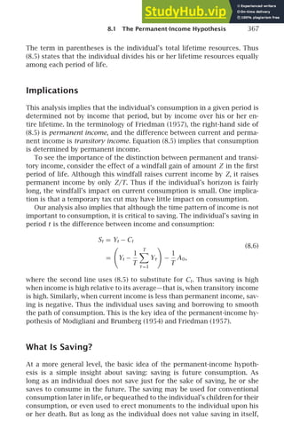
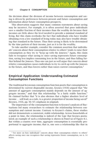
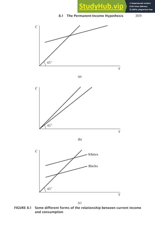
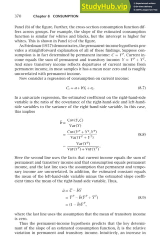
![8.1 The Permanent-Income Hypothesis 371
current income is associated with an increase in consumption only to the
extent that it reflects an increase in permanent income. When the variation in
permanent income is much greater than the variation in transitory income,
almost all differences in current income reflect differences in permanent in-
come; thus consumption rises nearly one-for-one with current income. But
when the variation in permanent income is small relative to the variation
in transitory income, little of the variation in current income comes from
variation in permanent income, and so consumption rises little with current
income.
This analysis can be used to understand the estimated consumption
functions in Figure 8.1. Across households, much of the variation in in-
come reflects such factors as unemployment and the fact that households
are at different points in their life cycles. As a result, the estimated slope
coefficient is substantially less than 1, and the estimated intercept is pos-
itive. Over time, in contrast, almost all the variation in aggregate income
reflects long-run growth—that is, permanent increases in the economy’s re-
sources. Thus the estimated slope coefficient is close to 1, and the estimated
intercept is close to zero.3
Now consider the differences between blacks and whites. The relative
variances of permanent and transitory income are similar in the two groups,
and so the estimates of b are similar. But blacks’ average incomes are lower
than whites’; as a result, the estimate of a for blacks is lower than the esti-
mate for whites (see [8.9]).
To see the intuition for this result, consider a member of each group
whose income equals the average income among whites. Since there are
many more blacks with permanent incomes below this level than there are
with permanent incomes above it, the black’s permanent income is much
more likely to be less than his or her current income than more. As a result,
blacks with this current income have on average lower permanent income;
thus on average they consume less than their income. For the white, in con-
trast, his or her permanent income is about as likely to be more than current
income as it is to be less; as a result, whites with this current income on
average have the same permanent income, and thus on average they con-
sume their income. In sum, the permanent-income hypothesis attributes
the different consumption patterns of blacks and whites to the different
average incomes of the two groups, and not to any differences in tastes or
culture.
3
In this case, although consumption is approximately proportional to income, the con-
stant of proportionality is less than 1; that is, consumption is on average less than permanent
income. As Friedman describes, there are various ways of extending the basic theory to make
it consistent with this result. One is to account for turnover among generations and long-run
growth: if the young generally save and the old generally dissave, the fact that each gener-
ation is wealthier than the previous one implies that the young’s saving is greater than the
old’s dissaving.](https://image.slidesharecdn.com/advanced-macroeconomics-230806183016-1212def2/85/Advanced-Macroeconomics-393-320.jpg)
![372 Chapter 8 CONSUMPTION
8.2 Consumption under Uncertainty:
The Random-Walk Hypothesis
Individual Behavior
We now extend our analysis to account for uncertainty. In particular, sup-
pose there is uncertainty about the individual’s labor income each period
(the Yt
′
S). Continue to assume that both the interest rate and the discount
rate are zero. In addition, suppose that the instantaneous utility function,
u(•), is quadratic. Thus the individual maximizes
E [U ] = E
T
t=1
Ct −
a
2
C2
t
, a 0. (8.10)
We will assume that the individual’s wealth is such that consumption is
always in the range where marginal utility is positive. As before, the indi-
vidual must pay off any outstanding debts at the end of life. Thus the budget
constraint is again given by equation (8.2),
T
t =1 Ct ≤ A0 +
T
t =1 Yt.
To describe the individual’s behavior, we use our usual Euler equation
approach. Specifically, suppose that the individual has chosen first-period
consumption optimally given the information available, and suppose that
he or she will choose consumption in each future period optimally given
the information then available. Now consider a reduction in C1 of dC from
the value the individual has chosen and an equal increase in consumption at
some future date from the value he or she would have chosen. If the individ-
ual is optimizing, a marginal change of this type does not affect expected
utility. Since the marginal utility of consumption in period 1 is 1 − aC1,
the change has a utility cost of (1 − aC1) dC. And since the marginal util-
ity of period-t consumption is 1 − aCt, the change has an expected utility
benefit of E1[1 − aCt] dC, where E1[•] denotes expectations conditional on
the information available in period 1. Thus if the individual is optimizing,
1 − aC1 = E1[1 − aCt], for t = 2, 3, . . . , T. (8.11)
Since E1[1 − aCt] equals 1 − aE1[Ct], this implies
C1 = E1[Ct], for t = 2, 3, . . . , T. (8.12)
The individual knows that his or her lifetime consumption will satisfy
the budget constraint, (8.2), with equality. Thus the expectations of the two
sides of the constraint must be equal:
T
t=1
E1[Ct] = A0 +
T
t=1
E1[Yt]. (8.13)](https://image.slidesharecdn.com/advanced-macroeconomics-230806183016-1212def2/85/Advanced-Macroeconomics-394-320.jpg)
![8.2 Consumption under Uncertainty: The Random-Walk Hypothesis 373
Equation (8.12) implies that the left-hand side of (8.13) is TC1. Substituting
this into (8.13) and dividing by T yields
C1 =
1
T
A0 +
T
t=1
E1[Yt]
. (8.14)
That is, the individual consumes 1/T of his or her expected lifetime
resources.
Implications
Equation (8.12) implies that the expectation as of period 1 of C2 equals C1.
More generally, reasoning analogous to what we have just done implies that
each period, expected next-period consumption equals current consump-
tion. This implies that changes in consumption are unpredictable. By the
definition of expectations, we can write
Ct = Et −1[Ct] + et, (8.15)
where et is a variable whose expectation as of period t − 1 is zero. Thus,
since Et −1[Ct] = Ct −1, we have
Ct = Ct −1 + et. (8.16)
This is Hall’s famous result that the permanent-income hypothesis implies
that consumption follows a random walk (Hall, 1978).4
The intuition for this
result is straightforward: if consumption is expected to change, the individ-
ual can do a better job of smoothing consumption. Suppose, for example,
that consumption is expected to rise. This means that the current marginal
utility of consumption is greater than the expected future marginal utility
of consumption, and thus that the individual is better off raising current
consumption. Thus the individual adjusts his or her current consumption
to the point where consumption is not expected to change.
In addition, our analysis can be used to find what determines the change
in consumption, e. Consider for concreteness the change from period 1 to
period 2. Reasoning parallel to that used to derive (8.14) implies that C2
4
Strictly speaking, the theory implies that consumption follows a martingale (a series
whose changes are unpredictable) and not necessarily a random walk (a martingale whose
changes are i.i.d.). The common practice, however, is to refer to martingales as random
walks.](https://image.slidesharecdn.com/advanced-macroeconomics-230806183016-1212def2/85/Advanced-Macroeconomics-395-320.jpg)
![374 Chapter 8 CONSUMPTION
equals 1/(T − 1) of the individual’s expected remaining lifetime resources:
C2 =
1
T − 1
A1 +
T
t=2
E2[Yt]
=
1
T − 1
A0 + Y1 − C1 +
T
t=2
E2[Yt]
,
(8.17)
where the second line uses the fact that A1 = A0 + Y1 − C1. We can rewrite
the expectation as of period 2 of income over the remainder of life,
T
t=2E2[Yt], as the expectation of this quantity as of period 1,
T
t=2E1[Yt],
plus the information learned between period 1 and period 2,
T
t=2E2[Yt] −
T
t=2E1[Yt]. Thus we can rewrite (8.17) as
C2 =
1
T − 1
A0 + Y1 − C1 +
T
t=2
E1[Yt] +
T
t=2
E2[Yt] −
T
t=2
E1[Yt]
. (8.18)
From (8.14), A0 + Y1 +
T
t=2E1[Yt] equals TC1. Thus (8.18) becomes
C2 =
1
T − 1
TC1 − C1 +
T
t=2
E2[Yt] −
T
t=2
E1[Yt]
(8.19)
= C1 +
1
T − 1
T
t=2
E2[Yt] −
T
t=2
E1[Yt]
.
Equation (8.19) states that the change in consumption between period 1 and
period 2 equals the change in the individual’s estimate of his or her lifetime
resources divided by the number of periods of life remaining.
Finally, note that the individual’s behavior exhibits certainty equivalence:
as (8.14) shows, the individual consumes the amount he or she would if his
or her future incomes were certain to equal their means; that is, uncertainty
about future income has no impact on consumption.
To see the intuition for this certainty-equivalence behavior, consider the
Euler equation relating consumption in periods 1 and 2. With a general in-
stantaneous utility function, this condition is
u′
(C1) = E1[u′
(C2)]. (8.20)
When utility is quadratic, marginal utility is linear. Thus the expected
marginal utility of consumption is the same as the marginal utility of ex-
pected consumption. That is, since E1[1 − aC2] = 1 − aE1[C2], for quadratic
utility (8.20) is equivalent to
u′
(C1) = u′
(E1[C2]). (8.21)
This implies C1 = E1[C2].](https://image.slidesharecdn.com/advanced-macroeconomics-230806183016-1212def2/85/Advanced-Macroeconomics-396-320.jpg)
![8.3 Two Tests of the Random-Walk Hypothesis 375
This analysis shows that quadratic utility is the source of certainty-
equivalence behavior: if utility is not quadratic, marginal utility is not lin-
ear, and so (8.21) does not follow from (8.20). We return to this point in
Section 8.6.5
8.3 Empirical Application: Two Tests of
the Random-Walk Hypothesis
Hall’s random-walk result ran strongly counter to existing views about con-
sumption.6
The traditional view of consumption over the business cycle
implies that when output declines, consumption declines but is expected to
recover; thus it implies that there are predictable movements in consump-
tion. Hall’s extension of the permanent-income hypothesis, in contrast, pre-
dicts that when output declines unexpectedly, consumption declines only
by the amount of the fall in permanent income; as a result, it is not expected
to recover.
Because of this divergence in the predictions of the two views, a great
deal of effort has been devoted to testing whether predictable changes in
income produce predictable changes in consumption. The hypothesis that
consumption responds to predictable income movements is referred to as
excess sensitivity of consumption (Flavin, 1981).7
Campbell and Mankiw’s Test Using Aggregate Data
The random-walk hypothesis implies that the change in consumption is un-
predictable; thus it implies that no information available at time t −1 can be
used to forecast the change in consumption from t − 1 to t. One approach
5
Although the specific result that the change in consumption has a mean of zero and is
unpredictable (equation [8.16]) depends on the assumption of quadratic utility (and on the
assumption that the discount rate and the interest rate are equal), the result that departures
of consumption growth from its average value are not predictable arises under more general
assumptions. See Problem 8.5.
6
Indeed, when Hall first presented the paper deriving and testing the random-walk result,
one prominent macroeconomist told him that he must have been on drugs when he wrote
the paper.
7
The permanent-income hypothesis also makes predictions about how consumption re-
sponds to unexpected changes in income. In the model of Section 8.2, for example, the
response to news is given by equation (8.19). The hypothesis that consumption responds
less than the permanent-income hypothesis predicts to unexpected changes in income is
referred to as excess smoothness of consumption. Since excess sensitivity concerns expected
changes in income and excess smoothness concerns unexpected changes, it is possible for
consumption to be excessively sensitive and excessively smooth at the same time. For more
on excess smoothness, see Campbell and Deaton (1989); West (1988); Flavin (1993); and
Problem 8.6.](https://image.slidesharecdn.com/advanced-macroeconomics-230806183016-1212def2/85/Advanced-Macroeconomics-397-320.jpg)


![384 Chapter 8 CONSUMPTION
is much larger at the end of life than at the beginning. But since labor in-
come is constant, this in turn implies that the individual gradually builds
up considerable savings over the first part of his or her life and gradually
decumulates them over the remainder. As a result, when horizons are finite
but long, wealth holdings may be highly responsive to the interest rate in
the long run even if the intertemporal elasticity of substitution is small.10
8.5 Consumption and Risky Assets
Individuals can invest in many assets, almost all of which have uncertain
returns. Extending our analysis to account for multiple assets and risk raises
some new issues concerning both household behavior and asset markets.
The Conditions for Individual Optimization
Consider an individual reducing consumption in period t by an infinitesimal
amount and using the resulting saving to buy an asset, i, that produces a
potentially uncertain stream of payoffs, Di
t +1, Di
t +2, . . . . If the individual is
optimizing, the marginal utility he or she forgoes from the reduced con-
sumption in period t must equal the expected sum of the discounted
marginal utilities of the future consumption provided by the asset’s pay-
offs. If we let P i
t denote the price of the asset, this condition is
u′
(Ct)P i
t = Et
∞
k=1
1
(1 + ρ)k
u′
(Ct +k)Di
t +k
for all i. (8.27)
To see the implications (8.27), suppose the individual holds the asset for
only one period, and define the return on the asset, ri
t +1, by ri
t +1 =
Di
t +1
P i
t
−1.
(Note that here the payoff to the asset, Di
t +1, includes not only any dividend
payouts in period t + 1, but also any proceeds from selling the asset.) Then
(8.27) becomes
u′
(Ct) =
1
1 + ρ
Et
1 + ri
t +1 u′
(Ct +1)
for all i. (8.28)
Since the expectation of the product of two variables equals the product of
their expectations plus their covariance, we can rewrite this expression as
u′
(Ct) =
1
1 + ρ
Et
1 + ri
t +1
Et [u′
(Ct +1)]
(8.29)
+ Covt 1 + ri
t +1,u′
(Ct +1)
for all i,
where Covt (•) is covariance conditional on information available at time t.
10
Carroll (1997) shows, however, that the presence of uncertainty weakens this
conclusion.](https://image.slidesharecdn.com/advanced-macroeconomics-230806183016-1212def2/85/Advanced-Macroeconomics-406-320.jpg)
![8.5 Consumption and Risky Assets 385
If we assume that utility is quadratic, u(C) = C−aC2
/2, then the marginal
utility of consumption is 1 − aC. Using this to substitute for the covariance
term in (8.29), we obtain
u′
(Ct) =
1
1 + ρ
Et
1 + ri
t +1
Et [u′
(Ct +1)] − aCovt 1 + ri
t +1,Ct +1
. (8.30)
Equation (8.30) implies that in deciding whether to hold more of an asset,
the individual is not concerned with how risky the asset is: the variance of
the asset’s return does not appear in (8.30). Intuitively, a marginal increase
in holdings of an asset that is risky, but whose risk is not correlated with
the overall risk the individual faces, does not increase the variance of the
individual’s consumption. Thus in evaluating that marginal decision, the
individual considers only the asset’s expected return.
Equation (8.30) implies that the aspect of riskiness that matters to the
decision of whether to hold more of an asset is the relation between the
asset’s payoff and consumption. Suppose, for example, that the individual
is given an opportunity to buy a new asset whose expected return equals
the rate of return on a risk-free asset that the individual is already able
to buy. If the payoff to the new asset is typically high when the marginal
utility of consumption is high (that is, when consumption is low), buying
one unit of the asset raises expected utility by more than buying one unit
of the risk-free asset. Thus (since the individual was previously indiffer-
ent about buying more of the risk-free asset), the individual can raise his
or her expected utility by buying the new asset. As the individual invests
more in the asset, his or her consumption comes to depend more on the
asset’s payoff, and so the covariance between consumption and the as-
set’s return becomes less negative. In the example we are considering, since
the asset’s expected return equals the risk-free rate, the individual invests
in the asset until the covariance of its return with consumption reaches
zero.
This discussion implies that hedging risks is crucial to optimal portfolio
choices. A steelworker whose future labor income depends on the health of
the U.S. steel industry should avoid—or better yet, sell short—assets whose
returns are positively correlated with the fortunes of the steel industry, such
as shares in U.S. steel companies. Instead the worker should invest in assets
whose returns move inversely with the health of the U.S. steel industry, such
as foreign steel companies or U.S. aluminum companies.
One implication of this analysis is that individuals should exhibit no
particular tendency to hold shares of companies that operate in the indi-
viduals’ own countries. In fact, because the analysis implies that individu-
als should avoid assets whose returns are correlated with other sources of
risk to their consumption, it implies that their holdings should be skewed
against domestic companies. For example, for plausible parameter values it
predicts that the typical person in the United States should sell U.S. stocks
short (Baxter and Jermann, 1997). In fact, however, individuals’ portfolios](https://image.slidesharecdn.com/advanced-macroeconomics-230806183016-1212def2/85/Advanced-Macroeconomics-407-320.jpg)
![386 Chapter 8 CONSUMPTION
are very heavily skewed toward domestic companies (French and Poterba,
1991). This pattern is known as home bias.
The Consumption CAPM
This discussion takes assets’ expected returns as given. But individuals’ de-
mands for assets determine these expected returns. If, for example, an as-
set’s payoff is highly correlated with consumption, its price must be driven
down to the point where its expected return is high for individuals to
hold it.
To see the implications of this observation for asset prices, suppose that
all individuals are the same, and return to the general first-order condition,
(8.27). Solving this expression for P i
t yields
P i
t = Et
∞
k=1
1
(1 + ρ)k
u′
(Ct +k)
u′
(Ct)
Di
t +k
. (8.31)
The term [1/(1 + ρ)k
]u′
(Ct +k)/u′
(Ct) shows how the consumer values future
payoffs, and therefore how much he or she is willing to pay for various
assets. It is referred to as the pricing kernel or stochastic discount factor.
Similarly, we can find the implications of our analysis for expected returns
by solving (8.30) for Et[1 + ri
t +1]:
Et
1 + ri
t +1
=
1
Et [u′
(Ct +1)]
(1 + ρ)u′
(Ct) + aCovt 1 + ri
t +1,Ct +1
. (8.32)
Equation (8.32) states that the higher the covariance of an asset’s payoff
with consumption, the higher its expected return must be.
We can simplify (8.32) by considering the return on a risk-free asset. If
the payoff to an asset is certain, then the covariance of its payoff with con-
sumption is zero. Thus the risk-free rate, rt +1, satisfies
1 + rt +1 =
(1 + ρ)u′
(Ct)
Et [u′
(Ct +1)]
. (8.33)
Subtracting (8.33) from (8.32) gives
Et
ri
t +1
− rt +1 =
aCovt 1 + ri
t +1, Ct +1
Et [u′
(Ct +1)]
. (8.34)
Equation (8.34) states that the expected-return premium that an asset must
offer relative to the risk-free rate is proportional to the covariance of its
return with consumption.
This model of the determination of expected asset returns is known
as the consumption capital-asset pricing model, or consumption CAPM. The](https://image.slidesharecdn.com/advanced-macroeconomics-230806183016-1212def2/85/Advanced-Macroeconomics-408-320.jpg)
![8.5 Consumption and Risky Assets 387
coefficient from a regression of an asset’s return on consumption growth
is known as its consumption beta. Thus the central prediction of the
consumption CAPM is that the premiums that assets offer are proportional
to their consumption betas (Breeden, 1979; see also Merton, 1973, and
Rubinstein, 1976).11
Empirical Application: The Equity-Premium Puzzle
One of the most important implications of this analysis of assets’ expected
returns concerns the case where the risky asset is a broad portfolio of
stocks. To see the issues involved, it is easiest to return to the Euler equation,
(8.28), and to assume that individuals have constant-relative-risk-aversion
utility rather than quadratic utility. With this assumption, the Euler equation
becomes
C −θ
t =
1
1 + ρ
Et
1 + ri
t +1 C −θ
t +1
, (8.35)
where θ is the coefficient of relative risk aversion. If we divide both sides
by C−θ
t and multiply both sides by 1 + ρ, this expression becomes
1 + ρ = Et
1 + ri
t +1
C −θ
t +1
C −θ
t
. (8.36)
Finally, it is convenient to let gc
t +1 denote the growth rate of consumption
from t to t + 1, (Ct +1/Ct) − 1, and to omit the time subscripts. Thus we have
E [(1 + ri
)(1 + gc
)−θ
] = 1 + ρ. (8.37)
To see the implications of (8.37), we take a second-order Taylor approx-
imation of the left-hand side around r = g = 0. Computing the relevant
derivatives yields
(1 + r)(1 + g)−θ
≃ 1 + r − θg − θgr + 1
2
θ(θ+ 1)g2
. (8.38)
Thus we can rewrite (8.37) as
E [ri
] − θE [gc
] − θ{E [ri
]E [gc
] + Cov(ri
,gc
)}
(8.39)
+ 1
2
θ(θ + 1){(E [gc
])2
+ Var(gc
)} ≃ ρ.
11
The original CAPM assumes that investors are concerned with the mean and variance of
the return on their portfolio rather than the mean and variance of consumption. That version
of the model therefore focuses on market betas—that is, coefficients from regressions of
assets’ returns on the returns on the market portfolio—and predicts that expected-return
premiums are proportional to market betas (Lintner, 1965, and Sharpe, 1964).](https://image.slidesharecdn.com/advanced-macroeconomics-230806183016-1212def2/85/Advanced-Macroeconomics-409-320.jpg)
![388 Chapter 8 CONSUMPTION
When the time period involved is short, the E [ri
]E [gc
] and (E [gc
])2
terms are
small relative to the others.12
Omitting these terms and solving the resulting
expression for E [ri
] yields
E [ri
] ≃ ρ + θE [gc
] + θCov(ri
,gc
) − 1
2
θ(θ+ 1)Var(gc
). (8.40)
Equation (8.40) implies that the difference between the expected returns on
two assets, i and j, satisfies
E [ri
] − E [r j
] = θCov(ri
,gc
) − θCov(r j
,gc
)
(8.41)
= θCov(ri
− r j
,gc
).
In a famous paper, Mehra and Prescott (1985) show that it is difficult
to reconcile observed returns on stocks and bonds with equation (8.41).
Mankiw and Zeldes (1991) report a simple calculation that shows the essence
of the problem. For the United States during the period 1890–1979 (which is
the sample that Mehra and Prescott consider), the difference between the av-
erage return on the stock market and the return on short-term government
debt—the equity premium—is about 6 percentage points. Over the same
period, the standard deviation of the growth of consumption (as measured
by real purchases of nondurables and services) is 3.6 percentage points, and
the standard deviation of the excess return on the market is 16.7 percentage
points; the correlation between these two quantities is 0.40. These figures
imply that the covariance of consumption growth and the excess return on
the market is 0.40(0.036)(0.167), or 0.0024.
Equation (8.41) therefore implies that the coefficient of relative risk aver-
sion needed to account for the equity premium is the solution to 0.06 =
θ(0.0024), or θ = 25. This is an extraordinary level of risk aversion; it
implies, for example, that individuals would rather accept a 17 percent
reduction in consumption with certainty than risk a 50-50 chance of a 20 per-
cent reduction. As Mehra and Prescott describe, other evidence suggests that
risk aversion is much lower than this. Among other things, such a high de-
gree of aversion to variations in consumption makes it puzzling that the
average risk-free rate is close to zero despite the fact that consumption is
growing over time.
Furthermore, the equity-premium puzzle has become more severe in the
period since Mehra and Prescott identified it. From 1979 to 2008, the aver-
age equity premium is 7 percentage points, which is slightly higher than in
Mehra and Prescott’s sample period. More importantly, consumption growth
has become more stable and less correlated with returns: the standard devi-
ation of consumption growth over this period is 1.1 percentage points, the
standard deviation of the excess market return is 14.2 percentage points,
and the correlation between these two quantities is 0.33. These figures
12
Indeed, for the continuous-time case, one can derive equation (8.40) without any
approximations.](https://image.slidesharecdn.com/advanced-macroeconomics-230806183016-1212def2/85/Advanced-Macroeconomics-410-320.jpg)
![8.6 Beyond the Permanent-Income Hypothesis 389
imply a coefficient of relative risk aversion of 0.07/[0.33(0.011)(0.142)], or
about 140.
The large equity premium, particularly when coupled with the low risk-
free rate, is thus difficult to reconcile with household optimization. This
equity-premium puzzle has stimulated a large amount of research, and many
explanations for it have been proposed. No clear resolution of the puzzle
has been provided, however.13
8.6 Beyond the Permanent-Income
Hypothesis
Background: Buffer-Stock Saving
The permanent-income hypothesis provides appealing explanations of many
important features of consumption. For example, it explains why temporary
tax cuts appear to have much smaller effects than permanent ones, and it
accounts for many features of the relationship between current income and
consumption, such as those described in Section 8.1.
Yet there are also important features of consumption that appear incon-
sistent with the permanent-income hypothesis. For example, as described
in Section 8.3, both macroeconomic and microeconomic evidence suggest
that consumption often responds to predictable changes in income. And as
we just saw, simple models of consumer optimization cannot account for
the equity premium.
Indeed, the permanent-income hypothesis fails to explain some central
features of consumption behavior. One of the hypothesis’s key predictions
is that there should be no relation between the expected growth of an indi-
vidual’s income over his or her lifetime and the expected growth of his or
her consumption: consumption growth is determined by the real interest
rate and the discount rate, not by the time pattern of income.
Carroll and Summers (1991) present extensive evidence that this predic-
tion of the permanent-income hypothesis is incorrect. For example, individ-
uals in countries where income growth is high typically have high rates of
consumption growth over their lifetimes, and individuals in slowly growing
countries typically have low rates of consumption growth. Similarly, typical
13
Proposed explanations include incomplete markets and transactions costs (Mankiw,
1986; Mankiw and Zeldes, 1991; Heaton and Lucas, 1996; Luttmer, 1999; and Problem 8.11);
habit formation (Constantinides, 1990; Campbell and Cochrane, 1999); nonexpected utility
(Weil, 1989b; Epstein and Zin, 1991; Bekaert, Hodrick, and Marshall, 1997); concern about
equity returns for reasons other than just their implications for consumption (Benartzi
and Thaler, 1995; Barberis, Huang, and Santos, 2001); gradual adjustment of consumption
(Gabaix and Laibson, 2001; Parker, 2001); and a small probability of a catastrophic decline
in consumption and equity prices (Barro, 2006).](https://image.slidesharecdn.com/advanced-macroeconomics-230806183016-1212def2/85/Advanced-Macroeconomics-411-320.jpg)

![8.6 Beyond the Permanent-Income Hypothesis 391
u′
(Ct) = Et [u′
(Ct +1)]. As described in Section 8.2, if utility is quadratic,
marginal utility is linear, and so Et [u′
(Ct +1)] equals u′
(Et [Ct +1]). Thus in this
case, the Euler equation reduces to Ct = Et [Ct +1]. But if u′′′
(•) is positive, then
u′
(C) is a convex function of C. In this case, Et [u′
(Ct +1)] exceeds u′
(Et [Ct +1]).
But this means that if Ct and Et [Ct +1] are equal, Et [u′
(Ct +1)] is greater than
u′
(Ct), and so a marginal reduction in Ct increases expected utility. Thus the
combination of a positive third derivative of the utility function and uncer-
tainty about future income reduces current consumption, and thus raises
saving. This saving is known as precautionary saving (Leland, 1968).
Panel (a) of Figure 8.3 shows the impact of uncertainty and a positive
third derivative of the utility function on the expected marginal utility of
consumption. Since u′′
(C) is negative, u′
(C) is decreasing in C. And since
u′′′
(C) is positive, u′
(C) declines less rapidly as C rises. If consumption takes
on only two possible values, CL and CH, each with probability 1
2
, the expected
marginal utility of consumption is the average of marginal utility at these
two values. In terms of the diagram, this is shown by the midpoint of the
line connecting u′
(CL) and u′
(CH). As the diagram shows, the fact that u′
(C)
is convex implies that this quantity is larger than marginal utility at the
average value of consumption, (CL + CH)/2.
Panel (b) depicts an increase in uncertainty. In particular, the low value
of consumption, CL, falls, and the high value, CH, rises, with no change in
their mean. When the high value of consumption rises, the fact that u′′′
(C) is
positive means that marginal utility falls relatively little; but when the low
value falls, the positive third derivative magnifies the rise in marginal utility.
As a result, the increase in uncertainty raises expected marginal utility for
a given value of expected consumption. Thus the increase in uncertainty
raises the incentive to save.
An important question, of course, is whether precautionary saving is
quantitatively important. To address this issue, recall equation (8.40) from
our analysis of the equity premium: E [ri
] ≃ ρ + θE [gc
] + θCov(ri
,gc
) −
1
2
θ(θ + 1)Var(gc
). If we consider a risk-free asset and assume r = ρ for
simplicity, this expression becomes
ρ ≃ ρ + θE [gc
] − 1
2
θ(θ + 1)Var(gc
), (8.42)
or
E [gc
] ≃ 1
2
(θ + 1)Var(gc
). (8.43)
Thus the impact of precautionary saving on expected consumption growth
depends on the variance of consumption growth and the coefficient of rel-
ative risk aversion.15
If both are substantial, precautionary saving can have
a large effect on expected consumption growth. If the coefficient of relative
risk aversion is 4 (which is toward the high end of values that are viewed
15
For a general utility function, the θ + 1 term is replaced by −Cu′′′
(C )/u′′
(C ). In anal-
ogy to the coefficient of relative risk aversion, −Cu′′
(C )/u′
(C ), Kimball (1990) refers to
−Cu′′′
(C )/u′′
(C ) as the coefficient of relative prudence.](https://image.slidesharecdn.com/advanced-macroeconomics-230806183016-1212def2/85/Advanced-Macroeconomics-413-320.jpg)
![392 Chapter 8 CONSUMPTION
u ′
(CL)
CL
CL
CH
CH
C
C
(a)
(CL + CH)/2
(CL + CH)/2
(b)
[u′
(CL ) + u′
(CH)]/2
u′
(CH)
u ′
(C)
u ′
(C)
[u′
(CL ) + u′
(CH)]/2
u′
([CL + CH]/2)
+ u ′
[u′
(CL )
′
(CH )]/2
′
CL
′
CH
′
FIGURE 8.3 The effects of a positive third derivative of the utility function on
the expected marginal utility of consumption
as plausible), and the standard deviation of households’ uncertainty about
their consumption 1 year ahead is 0.1 (which is consistent with the evidence
in Dynan, 1993, and Carroll, 1992), (8.43) implies that precautionary saving
raises expected consumption growth by 1
2
(4 + 1)(0. 1)2
, or 2.5 percentage
points.](https://image.slidesharecdn.com/advanced-macroeconomics-230806183016-1212def2/85/Advanced-Macroeconomics-414-320.jpg)
![394 Chapter 8 CONSUMPTION
These points can be seen in a three-period model. To distinguish the ef-
fects of liquidity constraints from precautionary saving, assume that the in-
stantaneous utility function is quadratic. In addition, continue to assume
that the real interest rate and the discount rate are zero.
Begin by considering the individual’s behavior in period 2. Let At denote
assets at the end of period t. Since the individual lives for only three periods,
C3 equals A2 + Y3, which in turn equals A1 + Y2 + Y3 − C2. The individual’s
expected utility over the last two periods of life as a function of his or her
choice of C2 is therefore
U = C2 − 1
2
aC2
2 + E2
(A1 + Y2 + Y3 − C2)
(8.44)
− 1
2
a(A1 + Y2 + Y3 − C2)2
.
The derivative of this expression with respect to C2 is
∂U
∂C2
= 1 − aC2 − (1 − aE2[A1 + Y2 + Y3 − C2])
(8.45)
= a(A1 + Y2 + E2[Y3] − 2C2).
This expression is positive for C2 (A1 + Y2 + E2[Y3])/2, and negative
thereafter. Thus, as we know from our earlier analysis, if the liquidity con-
straint does not bind, the individual chooses C2 = (A1 + Y2 + E2[Y3])/2. But
if it does bind, he or she sets consumption to the maximum attainable level,
which is A1 + Y2. Thus,
C2 = min
A1 + Y2 + E2[Y3]
2
,A1 + Y2
. (8.46)
Thus the liquidity constraint reduces current consumption if it is binding.
Now consider the first period. If the liquidity constraint is not binding
that period, the individual has the option of marginally raising C1 and paying
for this by reducing C2. Thus if the individual’s assets are not literally zero,
the usual Euler equation holds. With the specific assumptions we are mak-
ing, this means that C1 equals the expectation of C2.
But the fact that the Euler equation holds does not mean that the liquidity
constraints do not affect consumption. Equation (8.46) implies that if the
probability that the liquidity constraint will bind in the second period is
strictly positive, the expectation of C2 as of period 1 is strictly less than the
expectation of (A1 + Y2 + E2[Y3])/2. A1 is given by A0 + Y1 − C1, and the law
of iterated projections implies that E1[E2[Y3]] equals E1[Y3]. Thus,
C1
A0 + Y1 + E1[Y2] + E1[Y3] − C1
2
. (8.47)
Adding C1/2 to both sides of this expression and then dividing by 3
2
yields
C1
A0 + Y1 + E1[Y2] + E1[Y3]
3
. (8.48)](https://image.slidesharecdn.com/advanced-macroeconomics-230806183016-1212def2/85/Advanced-Macroeconomics-416-320.jpg)
![8.6 Beyond the Permanent-Income Hypothesis 395
Thus even when the liquidity constraint does not bind currently, the possi-
bility that it will bind in the future reduces consumption.
Finally, if the value of C1 that satisfies C1 = E1[C2] (given that C2 is deter-
mined by [8.46]) is greater than the individual’s period-1 resources, A0 +Y1,
the first-period liquidity constraint is binding; in this case the individual
consumes A0 + Y1.
Thus liquidity constraints alone, like precautionary saving alone, raise
saving. Explaining why household wealth is often low on the basis of liquid-
ity constraints therefore again requires appealing to a high discount rate.
As before, the high discount rate tends to make households want to have
high consumption. But with liquidity constraints, consumption cannot sys-
tematically exceed income early in life. Instead, households are constrained,
and so their consumption follows their income.
The combination of liquidity constraints and impatience can also explain
why households typically have some savings. When there are liquidity con-
straints, a household with no wealth faces asymmetric risks from increases
and decreases in income even if its utility is quadratic. A large fall in income
forces a corresponding fall in consumption, and thus a large rise in the
marginal utility of consumption. In contrast, a large rise in income causes
the household to save, and thus leads to only a moderate fall in marginal
utility. This is precisely the reason that the possibility of future liquidity
constraints lowers consumption. Researchers who have examined this issue
quantitatively, however, generally find that this effect is not large enough
to account for even the small savings we observe. Thus they typically in-
troduce a precautionary-saving motive as well. The positive third deriva-
tive of the utility function increases consumers’ desire to insure themselves
against the fall in consumption that would result from a fall in income, and
so increases the consumers’ savings beyond what would come about from
liquidity constraints and quadratic utility alone.17
Empirical Application: Credit Limits and Borrowing
In the absence of liquidity constraints, an increase in the amount a particular
lender is willing to lend will not affect consumption. But if there are bind-
ing liquidity constraints, such an increase will increase the consumption of
households that are borrowing as much as they can. Moreover, by making it
less likely that households will be up against their borrowing constraints in
the future, the increase may raise the consumption of households that are
not currently at their constraints.
17
Gourinchas and Parker (2002) extend the analysis of impatience, liquidity constraints,
and precautionary savings to the life cycle. Even a fairly impatient household wants to avoid
a large drop in consumption at retirement. Gourinchas and Parker find that as a result, it
appears that most households are mainly buffer-stock savers early in life but begin accu-
mulating savings for retirement once they reach middle age.](https://image.slidesharecdn.com/advanced-macroeconomics-230806183016-1212def2/85/Advanced-Macroeconomics-417-320.jpg)
![396 Chapter 8 CONSUMPTION
Gross and Souleles (2002) test these predictions by examining the im-
pact of changes in the credit limits on households’ credit cards. Their basic
regression takes the form:
Bit = b0 Lit + b1Li,t −1 + · · · + b12 Li,t −12 + a′
Xit + eit. (8.49)
Here i indexes households and t months, B is interest-incurring credit-card
debt, L is the credit limit, and X is a vector of control variables.
An obvious concern about equation (8.49) is that credit-card issuers might
tend to raise credit limits when cardholders are more likely to borrow more.
That is, there might be correlation between e, which captures other influ-
ences on borrowing, and the L terms. Gross and Souleles take various ap-
proaches to dealing with this problem. For example, in most specifications
they exclude cases where cardholders request increases in their borrowing
limits. Their most compelling approach uses institutional features of how
card issuers adjust credit limits that induce variation in L that is almost
certainly unrelated to variations in e. Most issuers are unlikely to raise a
card’s credit limit for a certain number of months after a previous increase,
with different issuers doing this for different numbers of months. Gross
and Souleles therefore introduce a set of dummy variables, D jn
, where D
jn
it
equals 1 if and only if household i’s card is from issuer j and i’s credit
limit was increased n months before month t. They then estimate (8.49) by
instrumental variables, using the D jn
’s as the instruments.
For Gross and Souleles’s basic instrumental-variables specification, the
sum of the estimated b’s in (8.49) is 0.111, with a standard error of 0.018.
That is, a one-dollar increase in the credit limit is associated with an 11-cent
increase in borrowing after 12 months. This estimate is highly robust to the
estimation technique, control variables, and sample.18
Gross and Souleles then ask whether the increased borrowing is confined
to households that are borrowing as much as they can. To do this, they split
the sample by the utilization rate (the ratio of the credit-card balance to the
credit limit) in month t −13 (the month before the earliest L term in [8.49]).
For households with initial utilization rates above 90 percent, the sum of the
b’s is very large: 0.452 (with a standard error of 0.125). Crucially, however,
it remains clearly positive for households with lower utilization rates: 0.158
(with a standard error of 0.060) when the utilization rate is between 50 and
90 percent, and 0.068 (with a standard error of 0.018) when the utilization
rate is less than 50 percent. Thus the data support not just the prediction
of the theory that changes in liquidity constraints matter for households
18
Gross and Souleles have data on borrowers’ other credit-card debt; they find no evi-
dence that the increased borrowing in response to the increases in credit limits lowers other
credit-card debt. However, since they do not have complete data on households’ balance
sheets, they cannot rule out the possibility that the increased borrowing is associated with
lower debt of other types or increased asset holdings. But they argue that since interest rates
on credit-card debt are quite high, this effect is unlikely to be large.](https://image.slidesharecdn.com/advanced-macroeconomics-230806183016-1212def2/85/Advanced-Macroeconomics-418-320.jpg)

![Problems 399
permanent-income hypothesis predict that estimated consumption functions
for farmers and nonfarmers differ?
8.3. The time-averaging problem. (Working, 1960.) Actual data give not con-
sumption at a point in time, but average consumption over an extended period,
such as a quarter. This problem asks you to examine the effects of this
fact.
Suppose that consumption follows a random walk: Ct = Ct −1 + et, where e
is white noise. Suppose, however, that the data provide average consumption
over two-period intervals; that is, one observes (Ct + Ct +1)/2, (Ct +2 + Ct +3)/2,
and so on.
(a) Find an expression for the change in measured consumption from one
two-period interval to the next in terms of the e’s.
(b) Is the change in measured consumption uncorrelated with the previous
value of the change in measured consumption? In light of this, is measured
consumption a random walk?
(c) Given your result in part (a), is the change in consumption from one two-
period interval to the next necessarily uncorrelated with anything known
as of the first of these two-period intervals? Is it necessarily uncorrelated
with anything known as of the two-period interval immediately preceding
the first of the two-period intervals?
(d ) Suppose that measured consumption for a two-period interval is not the
average over the interval, but consumption in the second of the two peri-
ods. That is, one observes Ct +1, Ct +3, and so on. In this case, is measured
consumption a random walk?
8.4. In the model of Section 8.2, uncertainty about future income does not affect
consumption. Does this mean that the uncertainty does not affect expected
lifetime utility?
8.5. (This follows Hansen and Singleton, 1983.) Suppose instantaneous utility is of
the constant-relative-risk-aversion form, u(Ct) = C1−θ
t /(1 − θ), θ 0. Assume
that the real interest rate, r, is constant but not necessarily equal to the dis-
count rate, ρ.
(a) Find the Euler equation relating Ct to expectations concerning Ct +1.
(b) Suppose that the log of income is distributed normally, and that as a
result the log of Ct +1 is distributed normally; let σ2
denote its variance
conditional on information available at time t. Rewrite the expression in
part (a) in terms of ln Ct, Et [ln Ct +1], σ2
, and the parameters r, ρ, and θ.
(Hint: If a variable x is distributed normally with mean µ and variance V,
E [ex
] = eµ
eV/2
.)
(c) Show that if r and σ2
are constant over time, the result in part (b) implies
that the log of consumption follows a random walk with drift: ln Ct +1 =
a + ln Ct + ut +1, where u is white noise.
(d ) How do changes in each of r and σ2
affect expected consumption growth,
Et [ln Ct +1 − ln Ct]? Interpret the effect of σ2
on expected consumption
growth in light of the discussion of precautionary saving in Section 8.6.](https://image.slidesharecdn.com/advanced-macroeconomics-230806183016-1212def2/85/Advanced-Macroeconomics-421-320.jpg)
![400 Chapter 8 CONSUMPTION
8.6. A framework for investigating excess smoothness. Suppose that Ct equals
[r/(1 + r)]{At +
∞
s =0
Et [Yt +s]/(1 + r)s
}, and that At +1 = (1 + r)(At + Yt − Ct).
(a) Show that these assumptions imply that Et [Ct +1] = Ct (and thus that
consumption follows a random walk) and that
∞
s=0
Et [Ct +s]/(1 + r)s
=
At +
∞
s=0
Et [Yt +s]/(1 + r)s
.
(b) Suppose that Yt = φYt −1 + ut, where u is white noise. Suppose that Yt
exceeds Et −1[Yt] by 1 unit (that is, suppose ut = 1). By how much does
consumption increase?
(c) For the case of φ 0, which has a larger variance, the innovation in
income, ut, or the innovation in consumption, Ct − Et −1[Ct]? Do consumers
use saving and borrowing to smooth the path of consumption relative to
income in this model? Explain.
8.7. Consider the two-period setup analyzed in Section 8.4. Suppose that the gov-
ernment initially raises revenue only by taxing interest income. Thus the in-
dividual’s budget constraint is C1 + C2/[1 + (1 − τ)r] ≤ Y1 + Y2/[1 + (1 − τ)r],
where τ is the tax rate. The government’s revenue is 0 in period 1 and
τr(Y1 − C0
1 ) in period 2, where C0
1 is the individual’s choice of C1 given this tax
rate. Now suppose the government eliminates the taxation of interest income
and instead institutes lump-sum taxes of amounts T1 and T2 in the two peri-
ods; thus the individual’s budget constraint is now C1 +C2/(1+r) ≤ (Y1 − T1)+
(Y2 − T2)/(1 + r). Assume that Y1, Y2, and r are exogenous.
(a) What condition must the new taxes satisfy so that the change does not
affect the present value of government revenues?
(b) If the new taxes satisfy the condition in part (a), is the old consumption
bundle, (C0
1 ,C0
2 ), not affordable, just affordable, or affordable with room to
spare?
(c) If the new taxes satisfy the condition in part (a), does first-period con-
sumption rise, fall, or stay the same?
8.8. Consider a stock that pays dividends of Dt in period t and whose price in period
t is Pt. Assume that consumers are risk-neutral and have a discount rate of r;
thus they maximize E [
∞
t =0
Ct/(1 + r)t
].
(a) Show that equilibrium requires Pt = Et [(Dt +1 + Pt +1)/(1 + r)] (assume that
if the stock is sold, this happens after that period’s dividends have been
paid).
(b) Assume that lims→∞ Et [Pt +s/(1 + r)s
] = 0 (this is a no-bubbles condition;
see the next problem). Iterate the expression in part (a) forward to derive
an expression for Pt in terms of expectations of future dividends.
8.9. Bubbles. Consider the setup of the previous problem without the assumption
that lims→∞ Et [Pt +s/(1 + r)s
] = 0.
(a) Deterministic bubbles. Suppose that Pt equals the expression derived in
part (b) of Problem 8.8 plus (1 + r)t
b, b 0.
(i) Is consumers’ first-order condition derived in part (a) of Problem 8.8
still satisfied?](https://image.slidesharecdn.com/advanced-macroeconomics-230806183016-1212def2/85/Advanced-Macroeconomics-422-320.jpg)
![Problems 401
(ii) Can b be negative? (Hint: Consider the strategy of never selling the
stock.)
(b) Bursting bubbles. (Blanchard, 1979.) Suppose that Pt equals the expres-
sion derived in part (b) of Problem 8.8 plus qt, where qt equals
(1 + r)qt −1/α with probability α and equals 0 with probability 1 − α.
(i) Is consumers’ first-order condition derived in part (a) of Problem 8.8
still satisfied?
(ii) If there is a bubble at time t (that is, if qt 0), what is the probability
that the bubble has burst by time t + s (that is, that qt +s = 0)? What is
the limit of this probability as s approaches infinity?
(c) Intrinsic bubbles. (Froot and Obstfeld, 1991.) Suppose that dividends fol-
low a random walk: Dt = Dt −1 + et, where e is white noise.
(i) In the absence of bubbles, what is the price of the stock in period t?
(ii) Suppose that Pt equals the expression derived in (i ) plus bt, where
bt = (1+r)bt −1 +cet, c 0. Is consumers’ first-order condition derived
in part (a) of Problem 8.8 still satisfied? In what sense do stock prices
overreact to changes in dividends?
8.10. The Lucas asset-pricing model. (Lucas, 1978.) Suppose the only assets in
the economy are infinitely lived trees. Output equals the fruit of the trees,
which is exogenous and cannot be stored; thus Ct = Yt, where Yt is the ex-
ogenously determined output per person and Ct is consumption per person.
Assume that initially each consumer owns the same number of trees. Since
all consumers are assumed to be the same, this means that, in equilibrium,
the behavior of the price of trees must be such that, each period, the repre-
sentative consumer does not want to either increase or decrease his or her
holdings of trees.
Let Pt denote the price of a tree in period t (assume that if the tree is
sold, the sale occurs after the existing owner receives that period’s output).
Finally, assume that the representative consumer maximizes E [
∞
t =0
ln Ct/
(1 + ρ)t
].
(a) Suppose the representative consumer reduces his or her consumption in
period t by an infinitesimal amount, uses the resulting saving to increase
his or her holdings of trees, and then sells these additional holdings in
period t + 1. Find the condition that Ct and expectations involving Yt +1,
Pt +1, and Ct +1 must satisfy for this change not to affect expected utility.
Solve this condition for Pt in terms of Yt and expectations involving Yt +1,
Pt +1, and Ct +1.
(b) Assume that lims→∞ Et [(Pt+s/Yt +s)/(1 + ρ)s
] = 0. Given this assumption,
iterate your answer to part (a) forward to solve for Pt. (Hint: Use the fact
that Ct+s = Yt +s for all s.)
(c) Explain intuitively why an increase in expectations of future dividends
does not affect the price of the asset.
(d ) Does consumption follow a random walk in this model?](https://image.slidesharecdn.com/advanced-macroeconomics-230806183016-1212def2/85/Advanced-Macroeconomics-423-320.jpg)
![402 Chapter 8 CONSUMPTION
8.11. The equity premium and the concentration of aggregate shocks. (Mankiw,
1986.) Consider an economy with two possible states, each of which occurs
with probability 1
2
. In the good state, each individual’s consumption is 1.
In the bad state, fraction λ of the population consumes 1 − (φ/λ) and the
remainder consumes 1, where 0 φ 1 and φ ≤ λ ≤ 1. φ measures the re-
duction in average consumption in the bad state, and λ measures how broadly
that reduction is shared.
Consider two assets, one that pays off 1 unit in the good state and one
that pays off 1 unit in the bad state. Let p denote the relative price of the
bad-state asset to the good-state asset.
(a) Consider an individual whose initial holdings of the two assets are zero,
and consider the experiment of the individual marginally reducing (that
is, selling short) his or her holdings of the good-state asset and using the
proceeds to purchase more of the bad-state asset. Derive the condition
for this change not to affect the individual’s expected utility.
(b) Since consumption in the two states is exogenous and individuals are
ex ante identical, p must adjust to the point where it is an equilibrium
for individuals’ holdings of both assets to be zero. Solve the condition
derived in part (a) for this equilibrium value of p in terms of φ, λ, U ′
(1),
and U ′
(1 − (φ/λ)).
(c) Find ∂p/∂λ.
(d) Show that if utility is quadratic, ∂p/∂λ = 0.
(e) Show that if U ′′′
(•) is everywhere positive, ∂p/∂λ 0.
8.12. Consumption of durable goods. (Mankiw, 1982.) Suppose that, as in Sec-
tion 8.2, the instantaneous utility function is quadratic and the interest rate
and the discount rate are zero. Suppose, however, that goods are durable;
specifically, Ct = (1 − δ)Ct −1 + Xt, where Xt is purchases in period t and
0 ≤ δ 1.
(a) Consider a marginal reduction in purchases in period t of dX t. Find values
of dX t +1 and dX t +2 such that the combined changes in Xt, Xt +1, and
Xt +2 leave the present value of spending unchanged (so dX t + dX t +1 +
dX t +2 = 0) and leave Ct +2 unchanged (so (1 − δ)2
dXt + (1 − δ)dX t +1 +
dX t +2 = 0).
(b) What is the effect of the change in part (a) on Ct and Ct +1? What is the
effect on expected utility?
(c) What condition must Ct and Et [Ct +1] satisfy for the change in part (a)
not to affect expected utility? Does C follow a random walk?
(d ) Does X follow a random walk? (Hint: Write Xt − Xt −1 in terms of Ct −Ct −1
and Ct −1 − Ct−2.) Explain intuitively. If δ = 0, what is the behavior of X?
8.13. Habit formation and serial correlation in consumption growth. Suppose
that the utility of the representative consumer, individual i, is given by
T
t=1
[1/(1 + ρ)t
](Cit/Zit)1−θ
/(1 − θ), ρ 0, θ 0, where Zit is the “reference”
level of consumption. Assume the interest rate is constant at some level, r,
and that there is no uncertainty.](https://image.slidesharecdn.com/advanced-macroeconomics-230806183016-1212def2/85/Advanced-Macroeconomics-424-320.jpg)


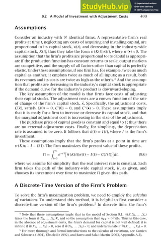
![410 Chapter 9 INVESTMENT
objective function is
=
∞
t =0
1
(1 + r)t
[π(Kt)κt − It − C(It)]. (9.7)
For comparability with the continuous-time case, it is helpful to assume that
the firm’s investment and its capital stock are related by κt = κt −1 + It for
all t.6
We can think of the firm as choosing its investment and capital stock
each period subject to the constraint κt = κt −1 + It for each t. Since there
are infinitely many periods, there are infinitely many constraints.
The Lagrangian for the firm’s maximization problem is
L =
∞
t =0
1
(1 + r)t
[π(Kt)κt − It − C(It)] +
∞
t =0
λt (κt −1 + It − κt). (9.8)
λt is the Lagrange multiplier associated with the constraint relating κt and
κt −1. It therefore gives the marginal value of relaxing the constraint; that is,
it gives the marginal impact of an exogenous increase in κt on the lifetime
value of the firm’s profits discounted to time 0. This discussion implies
that if we define qt = (1 + r)t
λt, then qt shows the value to the firm of an
additional unit of capital at time t in time-t dollars. With this definition, we
can rewrite the Lagrangian as
L′
=
∞
t =0
1
(1 + r)t
[π(Kt)κt − It − C(It) + qt(κt −1 + It − κt)]. (9.9)
The first-order condition for the firm’s investment in period t is therefore
1
(1 + r)t
[−1 − C′
(It) + qt] = 0, (9.10)
which is equivalent to
1 + C′
(It) = qt. (9.11)
To interpret this condition, observe that the cost of acquiring a unit of cap-
ital equals the purchase price (which is fixed at 1) plus the marginal adjust-
ment cost. Thus (9.11) states that the firm invests to the point where the
cost of acquiring capital equals the value of the capital.
Now consider the first-order condition for capital in period t. The term
for period t in the Lagrangian, (9.9), involves both κt and κt −1. Thus the
capital stock in period t, κt, appears in both the term for period t and the
6
The more standard assumption is κt = κt −1 + It−1. However, this formulation imposes
a one-period delay between investment and the resulting increase in capital that has no
analogue in the continuous-time case.](https://image.slidesharecdn.com/advanced-macroeconomics-230806183016-1212def2/85/Advanced-Macroeconomics-432-320.jpg)
![9.2 A Model of Investment with Adjustment Costs 411
term for period t + 1. The first-order condition for κt is therefore
1
(1 + r)t
[π(Kt) − qt] +
1
(1 + r)t +1
qt +1 = 0. (9.12)
Multiplying this expression by (1 + r)t +1
and rearranging yields
(1 + r)π(Kt) = (1 + r)qt − qt +1. (9.13)
If we define qt = qt +1 − qt, we can rewrite the right-hand side of (9.13) as
rqt − qt. Thus we have
π(Kt) =
1
1 + r
(rqt − qt). (9.14)
The left-hand side of (9.14) is the marginal revenue product of capital, and
the right-hand side is the opportunity cost of a unit of capital. Intuitively,
owning a unit of capital for a period requires forgoing rqt of real interest
and involves offsetting capital gains of qt (see [9.4] with the depreciation
rate assumed to be zero; in addition, there is a factor of 1/(1 + r) that will
disappear in the continuous-time case). For the firm to be optimizing, the
returns to capital must equal this opportunity cost. This is what is stated
by (9.14). This condition is thus analogous to the condition in the model
without adjustment costs that the firm rents capital to the point where its
marginal revenue product equals its rental price.
A second way of interpreting (9.14) is as a consistency requirement con-
cerning how the firm values capital over time. To see this interpretation,
rearrange (9.14) (or [9.13]) as
qt = π(Kt) +
1
1 + r
qt +1. (9.15)
By definition, qt is the value the firm attaches to a unit of capital in period t
measured in period-t dollars, and qt +1 is the value the firm will attach to
a unit of capital in period t + 1 measured in period-(t + 1) dollars. If qt
does not equal the amount the capital contributes to the firm’s objective
function this period, π(Kt), plus the value the firm will attach to the capital
next period measured in this period’s dollars, qt +1/(1 + r), its valuations in
the two periods are inconsistent.
Conditions (9.11) and (9.15) are not enough to completely characterize
profit-maximizing behavior, however. The problem is that although (9.15)
requires the q’s to be consistent over time, it does not require them to
actually equal the amount that an additional unit of capital contributes to
the firm’s objective function. To see this, suppose the firm has an additional
unit of capital in period 0 that it holds forever. Since the additional unit of
capital raises profits in period t by π(Kt), we can write the amount the capital](https://image.slidesharecdn.com/advanced-macroeconomics-230806183016-1212def2/85/Advanced-Macroeconomics-433-320.jpg)
![412 Chapter 9 INVESTMENT
contributes to the firm’s objective function as
MB = lim
T→∞
T−1
t =0
1
(1 + r)t
π(Kt) . (9.16)
Now note that equation (9.15) implies that q0 can be written as
q0 = π(K0) +
1
1 + r
q1
= π(K0) +
1
1 + r
π(K1) +
1
1 + r
q2
= . . .
= lim
T→∞
T−1
t =0
1
(1 + r)t
π(Kt) +
1
(1 + r)T
qT ,
(9.17)
where the first line uses (9.15) for t = 0, and the second uses it for t = 1.
Comparison of (9.16) and (9.17) shows that q0 equals the contribution of
an additional unit of capital to the firm’s objective function if and only if
lim
T→∞
1
(1 + r)T
qT = 0. (9.18)
If (9.18) fails, then marginally raising investment in period 0 (which, by
[9.11], has a marginal cost of q0) and holding the additional capital forever
(which has a marginal benefit of MB) has a nonzero impact on the firm’s
profits, which would mean that the firm is not maximizing profits. Equa-
tion (9.18) is therefore necessary for profit maximization. This condition is
known as the transversality condition.
An alternative version of the transversality condition is
lim
T→∞
1
(1 + r)T
qTκT = 0. (9.19)
Intuitively, this version of the condition states that it cannot be optimal to
hold valuable capital forever. In the model we are considering, κ̇ and q are
linked through (9.11), and so κ diverges if and only if q does. One can show
that as a result, (9.19) holds if and only if (9.18) does. Thus we can use either
condition.
The Continuous-Time Case
We can now consider the case when time is continuous. The firm’s profit-
maximizing behavior in this case is characterized by three conditions that
are analogous to the three conditions that characterize its behavior in dis-
crete time: (9.11), (9.14), and (9.19). Indeed, the optimality conditions for
continuous time can be derived by considering the discrete-time problem](https://image.slidesharecdn.com/advanced-macroeconomics-230806183016-1212def2/85/Advanced-Macroeconomics-434-320.jpg)
![9.2 A Model of Investment with Adjustment Costs 413
where the time periods are separated by intervals of length t and then tak-
ing the limit as t approaches zero. We will not use this method, however.
Instead we will simply describe how to find the optimality conditions, and
justify them as necessary by way of analogy to the discrete-time case.
The firm’s problem is now to maximize the continuous-time objective
function, (9.6), rather than the discrete-time objective function, (9.7).
The first step in analyzing this problem is to set up the current-value
Hamiltonian:
H (κ(t),I (t)) = π(K(t))κ(t) − I (t) − C(I (t)) + q(t)I (t). (9.20)
This expression is analogous to the period-t term in the Lagrangian for the
discrete-time case with the term in the change in the capital stock omitted
(see [9.9]). There is some standard terminology associated with this type of
problem. The variable that can be controlled freely (I ) is the control variable;
the variable whose value at any time is determined by past decisions (κ) is
the state variable; and the shadow value of the state variable (q) is the costate
variable.
The first condition characterizing the optimum is that the derivative of
the Hamiltonian with respect to the control variable at each point in time is
zero. This is analogous to the condition in the discrete-time problem that
the derivative of the Lagrangian with respect to I for each t is zero. For our
problem, this condition is
1 + C ′
(I (t)) = q(t). (9.21)
This condition is analogous to (9.11) in the discrete-time case.
The second condition is that the derivative of the Hamiltonian with re-
spect to the state variable equals the discount rate times the costate variable
minus the derivative of the costate variable with respect to time. In our case,
this condition is
π(K(t)) = rq(t) − ˙
q (t). (9.22)
This condition is analogous to (9.14) in the discrete-time problem.
The final condition is the continuous-time version of the transversality
condition. This condition is that the limit of the product of the discounted
costate variable and the state variable is zero. In our model, this condition is
lim
t→∞
e−r t
q(t)κ(t) = 0. (9.23)
Equations (9.21), (9.22), and (9.23) characterize the firm’s behavior.7
7
An alternative approach is to formulate the present-value Hamiltonian, H̃ (κ(t),I (t)) =
e−rt
[π (K(t))κ(t) − I (t) − C (I (t))] + λ(t)I (t). This is analogous to using the Lagrangian (9.8)
rather than (9.9). With this formulation, (9.22) is replaced by e−rt
π (K(t)) = −λ̇(t), and (9.23)
is replaced by limt→∞ λ(t)κ(t) = 0.](https://image.slidesharecdn.com/advanced-macroeconomics-230806183016-1212def2/85/Advanced-Macroeconomics-435-320.jpg)
![414 Chapter 9 INVESTMENT
9.3 Tobin’s q
Our analysis of the firm’s maximization problem implies that q summarizes
all information about the future that is relevant to a firm’s investment deci-
sion. q shows how an additional dollar of capital affects the present value
of profits. Thus the firm wants to increase its capital stock if q is high and
reduce it if q is low; the firm does not need to know anything about the
future other than the information that is summarized in q in order to make
this decision (see [9.21]).
From our analysis of the discrete-time case, we know that q is the present
discounted value of the future marginal revenue products of a unit of capi-
tal. In the continuous-time case, we can therefore express q as
q(t) =
∞
τ=t
e−r (τ−t )
π(K(τ)) dτ. (9.24)
There is another interpretation of q. A unit increase in the firm’s capital
stock increases the present value of the firm’s profits by q, and thus raises
the value of the firm by q. Thus q is the market value of a unit of capital. If
there is a market for shares in firms, for example, the total value of a firm
with one more unit of capital than another firm exceeds the value of the
other by q. And since we have assumed that the purchase price of capital
is fixed at 1, q is also the ratio of the market value of a unit of capital to
its replacement cost. Thus equation (9.21) states that a firm increases its
capital stock if the market value of capital exceeds the cost of acquiring it,
and that it decreases its capital stock if the market value of the capital is
less than the cost of acquiring it.
The ratio of the market value to the replacement cost of capital is known
as Tobin’s q (Tobin, 1969); it is because of this terminology that we used q to
denote the value of capital in the previous section. Our analysis implies that
what is relevant to investment is marginal q—the ratio of the market value
of a marginal unit of capital to its replacement cost. Marginal q is likely to
be harder to measure than average q—the ratio of the total value of the
firm to the replacement cost of its total capital stock. Thus it is important
to know how marginal q and average q are related.
One can show that in our model, marginal q is less than average q. The
reason is that when we assumed that adjustment costs depend only on κ̇,
we implicitly assumed diminishing returns to scale in adjustment costs. Our
assumptions imply, for example, that it is more than twice as costly for a
firm with 20 units of capital to add 2 more than it is for a firm with 10 units
to add 1 more. Because of this assumption of diminishing returns, firms’
lifetime profits, , rise less than proportionally with their capital stocks,](https://image.slidesharecdn.com/advanced-macroeconomics-230806183016-1212def2/85/Advanced-Macroeconomics-436-320.jpg)
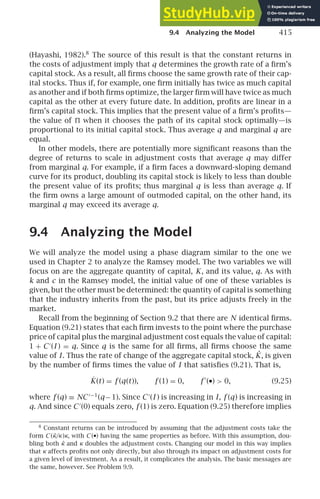
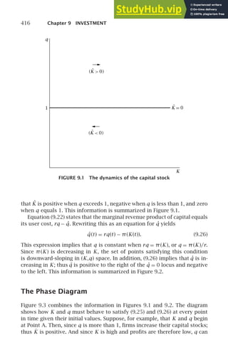
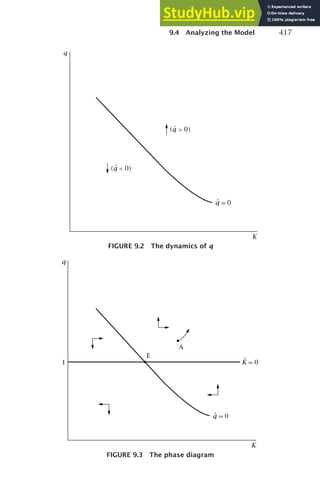
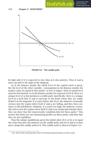
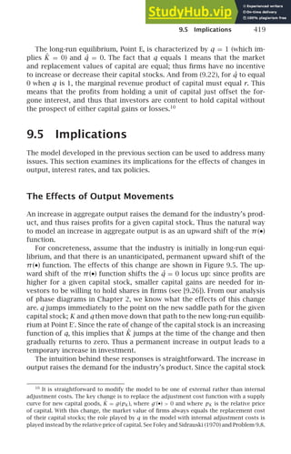
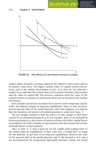
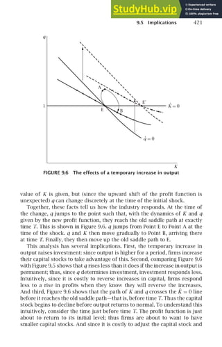

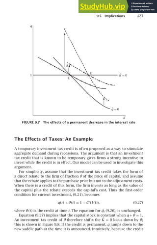
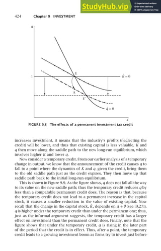
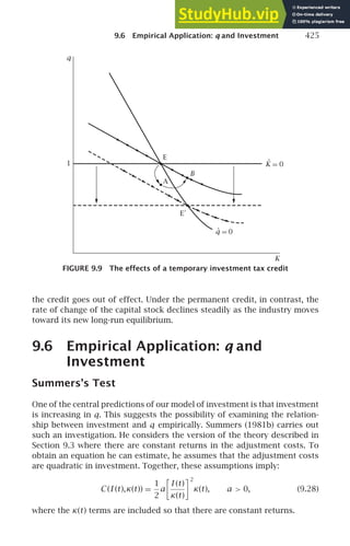
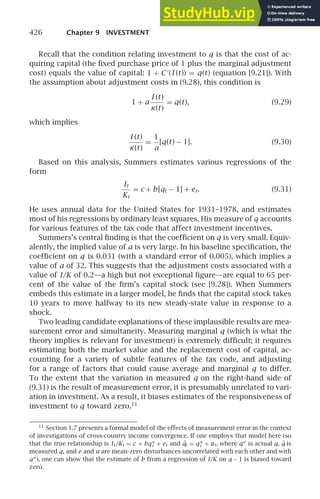

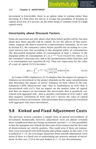

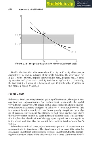
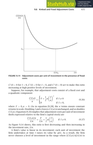


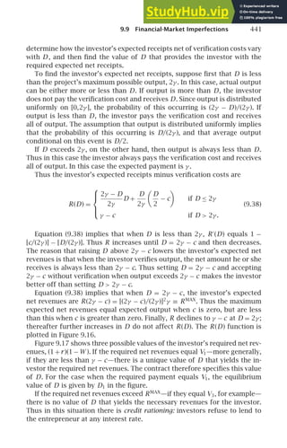
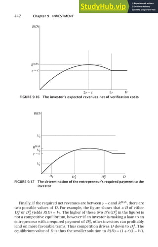
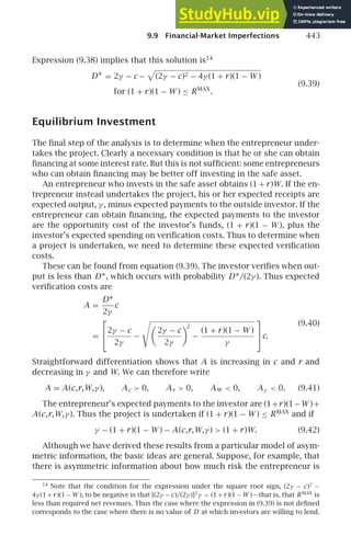
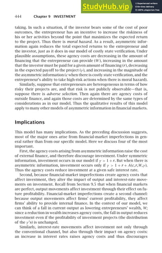

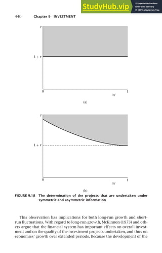


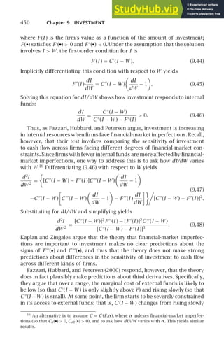
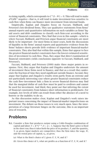
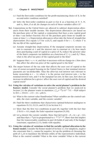
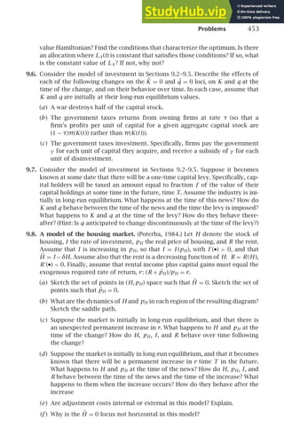


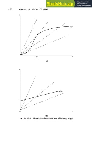
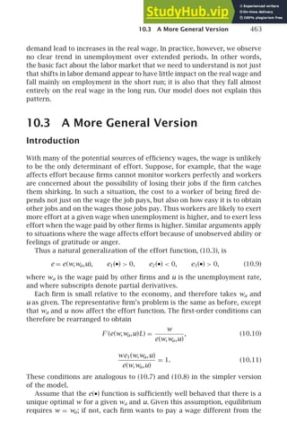
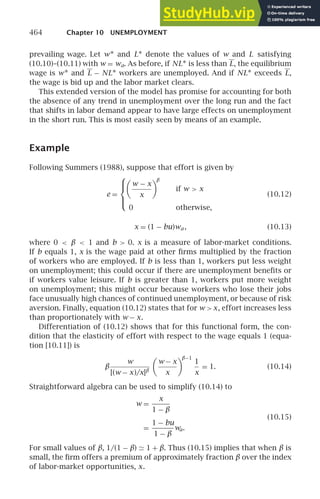
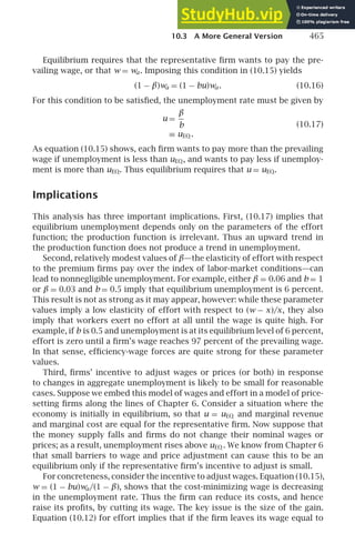

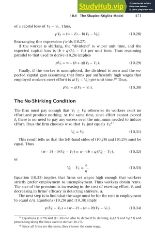
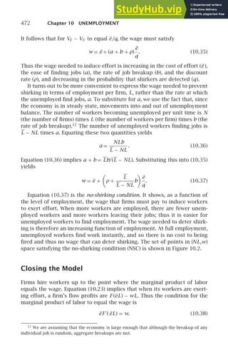
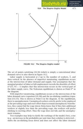
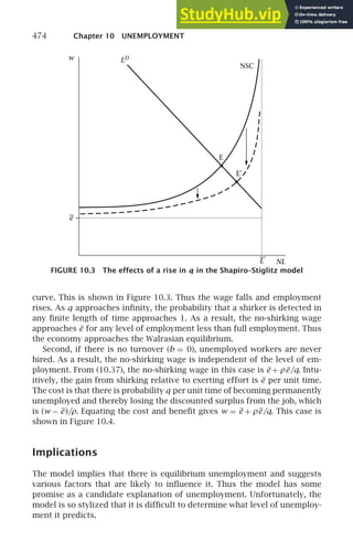
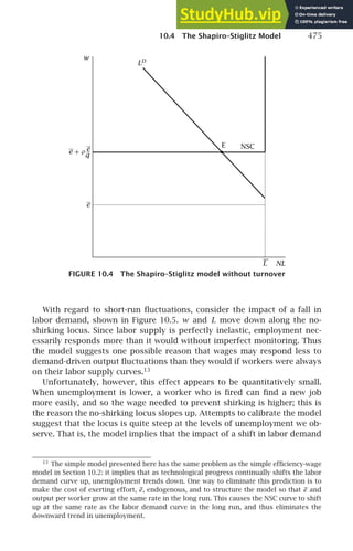
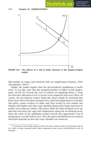


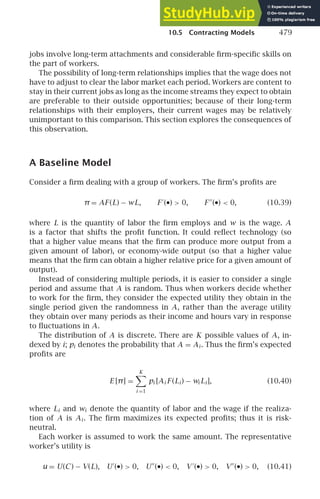

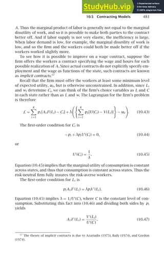


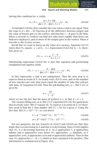
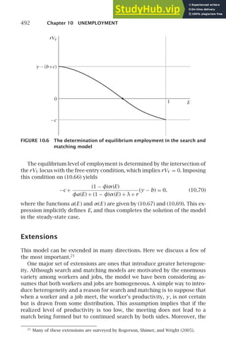


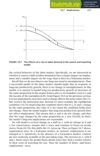
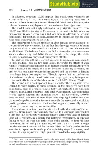
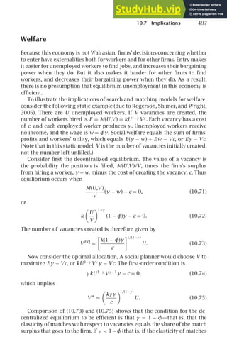

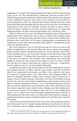
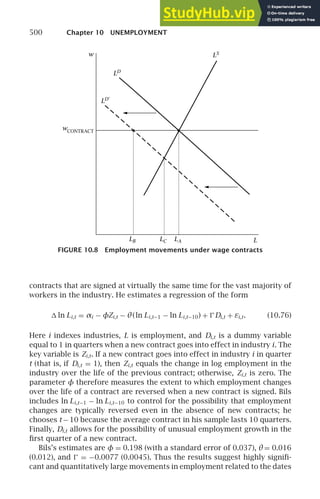


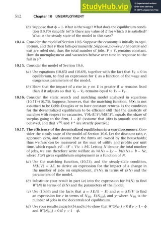
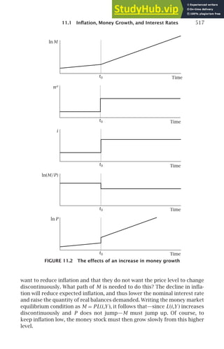
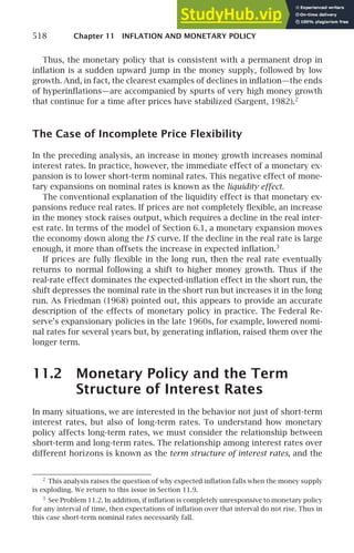
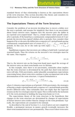

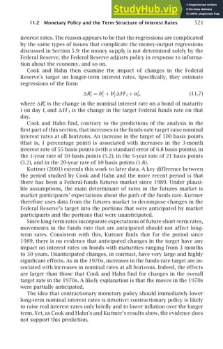


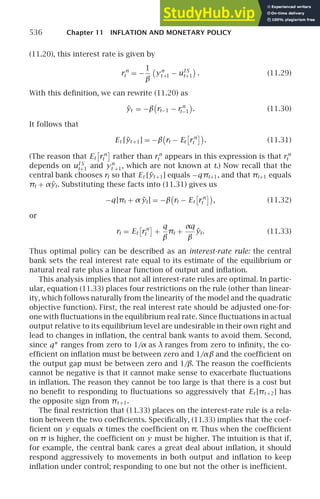
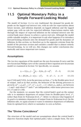
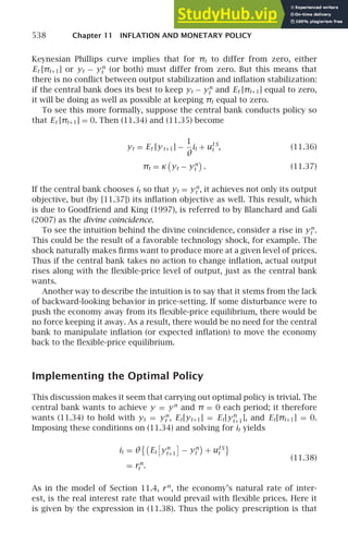
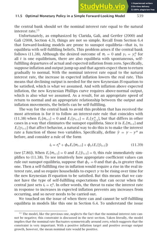


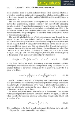
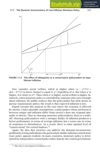

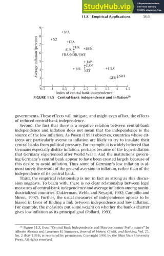
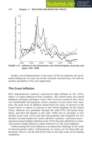


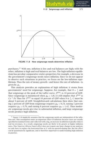
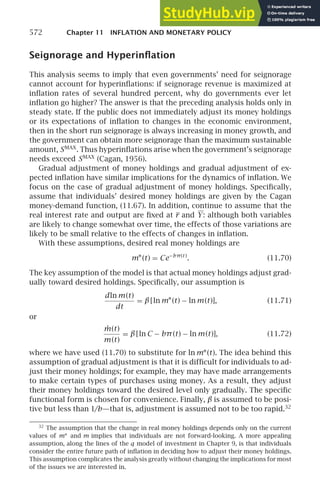
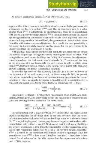
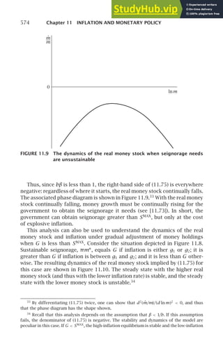
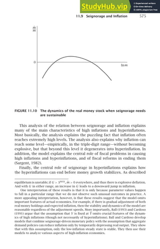


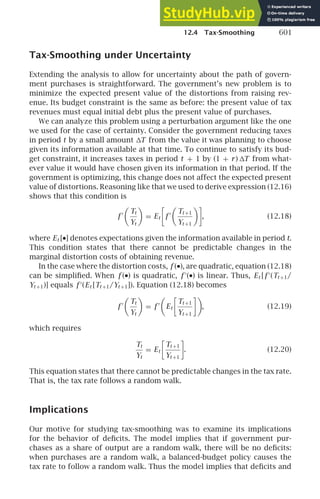


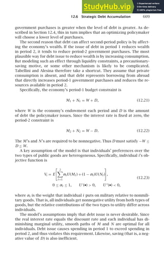

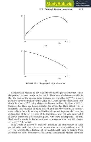

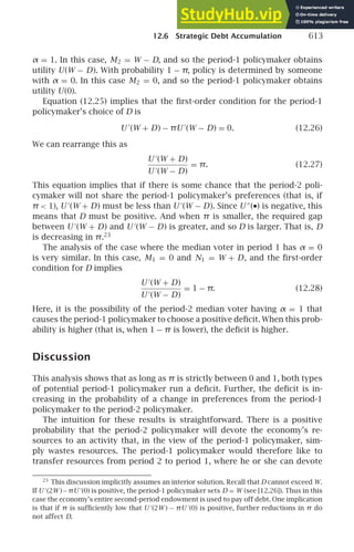


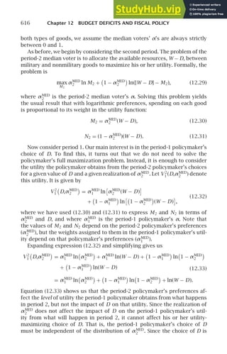


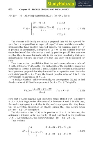
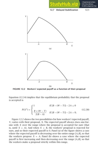
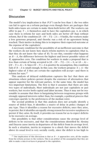


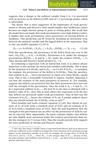


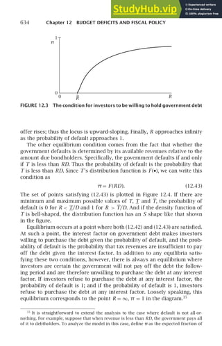
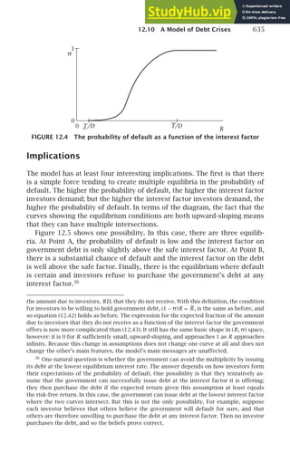
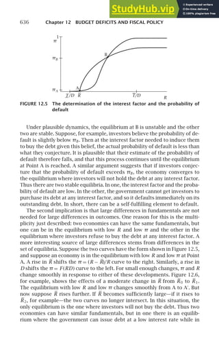


This document provides the table of contents for a textbook on advanced macroeconomics. The textbook is organized into 12 chapters covering various macroeconomic models and topics, including economic growth, business cycles, consumption, investment, unemployment, inflation, and fiscal policy. It also includes an epilogue on the 2008 financial crisis. Several chapters include empirical applications sections that discuss real-world evidence related to the theoretical models presented.


