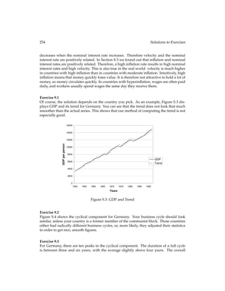
This document provides a preface and table of contents for a book on macroeconomics. The preface describes the book's purpose as a supplement to another macroeconomics textbook that uses more intuitive and graphical explanations rather than formal models. This book aims to work out more concrete formal models using students' calculus skills. It describes the book's organization and alignment with the other textbook's chapters. It also provides information on teaching the material, exercises included, acknowledgements, and contact information for the authors.

1. MACROECONOMICS
1880 1900 1920 1940 1960 1980 2000
Matthias Doepke
University of Chicago
Andreas Lehnert
Board of Governors of the
Federal Reserve System
Andrew W. Sellgren
George Mason University

2. This book was typeset in Palatino and Computer Modern using L
A
TEX.
Draft of 1 September 1999.
Chapters 5, 8, 9, and 11 Copyright c
1999, by Matthias Doepke.
Chapters 10, 12, 13, 14, 17, 18, and 19 Copyright c
1999, by Andreas Lehnert.
Chapters 1, 2, 3, 4, 6, and 15 Copyright c
1999, by Andrew W. Sellgren.
All rights reserved. No part of this work may be reproduced in any form by any electronic
or mechanical means (including, but not limited to, photocopying, recording, or informa-
tion storage and retrieval) without permission in writing from the copyright owner.
The authors permit faculty, students, and staff of the University of Chicago to copy and
distribute any part of this work for use in classes taught at the University of Chicago.

3. Preface
We have designed this book to be a supplement to Robert J. Barro’s Macroeconomics, which
is the textbook that is used in introductory macroeconomics courses at the University of
Chicago. In teaching these courses, we have found that Barro’s treatment of the subject
does not make use of the mathematical skills of our students. In particular, Barro relies
almost exclusively on economic intuition and graphs to elucidate his subject. Since our
students are familiar with calculus, we are able to work out formal models. This almost
always allows greater concreteness and concision.
We have attempted to align our chapters with those in Barro’s textbook. Sometimes our
chapters present mathematical versions of the models that Barro introduces in his corre-
sponding chapters (as in Chapters 2 and 19). Other times, our chapters contain material
that extends his work (as in Chapters 5 and 17). Throughout, we have tried to add value to
the treatment in Barro’s book and to minimize redundancy. For example, we have nothing
to add to Barro’s Chapters 7, 16, and 20, so we have not covered those chapters. Three
chapters deviate from this plan. Chapter 1 develops the mathematics of interest rates and
growth rates; Barro does not cover these topics, but they are behind the scenes in his Chap-
ter 1 and throughout his book. Chapter 10, which covers unemployment, is completely
unrelated to Barro’s Chapter 10. It is intended as a companion to the book Job Creation and
Destruction by Davis, Haltiwanger, and Schuh. Chapter 18 covers the relationship between
the government budget constraint and inflation along the lines of the “Unpleasant Mon-
etarist Arithmetic” of Sargent and Wallace. Although Barro has a sidebar on this topic in
his Chapter 14, we feel that it is important enough to merit a chapter of its own. We chose
Chapter 18 since it is a natural point between fiscal policy (Chapters 12, 13, and 14) and
monetary policy (Chapter 19). Barro’s Chapter 18 is a review of the empirical evidence on
the effect of monetary shocks on the real economy, and is well worth covering.
There are exercises after each chapter, and we have provided complete solutions at the
end of this book. We believe that exercises are essential for students to learn this material.
They give students a sense of what they ought to know, since these exercises have been
drawn from several years of exams. Also, we often use exercises to introduce extensions
to the material in the text. We have attempted to estimate the difficulty of these exercises,
labeling them as “Easy,” “Moderate”, or “Hard”. An exercise with a “Hard” rating may
require a lot of algebra, or it may use unfamiliar concepts. Most other questions are rated

4. iv Preface
as “Moderate”, unless they have one-line solutions, in which case we usually rated them
as “Easy”.
We teach this material in two ten-week courses. In the first course we cover Chapters 1, 2,
3, 6, 4, 5, 7, 8, 9, and 11, in that order. This allows us to keep together all the material on
monetary economics (Chapters 4, 5, 7, and 8). In the second course, we cover Chapter 10
(unemployment); Chapters 12, 13, and 14 (fiscal policy); Chapters 15 and 16 (international
macro); and Chapters 17, 18 and 19 (money and banking). Since this is quite a lot to cover
in ten weeks, instructors of the second course have traditionally touched only briefly on
unemployment and international macro and concentrated instead on monetary and fiscal
policy. The second course can benefit substantially from outside readings, such as: Rational
Expectations and Inflation by Thomas Sargent; A Monetary History of the United States by Mil-
ton Friedman and Anna Schwartz; and Job Creation and Destruction by Davis, Haltiwanger,
and Schuh.
This book would not have been possible without the support of the Department of Eco-
nomics at the University of Chicago and the encouragement of Grace Tsiang. We would
also like to thank the many students and faculty who have helped us to develop this ma-
terial. A number of exercises in the first half of the book were based on questions written
by Robert E. Lucas, Jr. The material in the second half of this book has benefited from sev-
eral generations of instructors of Economics 203. In particular, Alexander Reyfman wrote
a series of lectures which were the genesis of Chapters 12 through 19. Reyfman’s teach-
ing assistant Bill Dupor, and Lehnert’s teaching assistants Jerry Cubbin and Tom Miles,
all contributed valuable suggestions. During Cubbin’s tenure as TA, he wrote most of the
solutions to the problem sets, and several of these have found their way into this book. All
students subjected to early drafts of this material contributed to the book’s current form;
Shannon Thaden, Ben Ruff, and Calvin Chan deserve special mention.
In spite of all the comments and suggestions we have received, this book inevitably con-
tains errors and omissions. We would be grateful if you would bring these to our attention.
The authors can be reached by e-mail at:
m-doepke@uchicago.edu
There is also a tear-out feedback form at the end of the book, along with a tear-out midterm-
evaluation form for Economics 202 and 203.
Finally, some of the material in this book involves policy prescriptions. At some level,
policy is a matter of opinion. The opinions expressed herein are not necessarily those of
the Board of Governors of the Federal Reserve System.
Chicago, Illinois
September 1999

5. Contents
Preface iii
1 Preliminaries 1
1.1 Compound Interest . . . . . . . . . . . . . . . . . . . . . . . . . . . . . . . . . 1
1.2 Growth Rates . . . . . . . . . . . . . . . . . . . . . . . . . . . . . . . . . . . . 3
Exercises . . . . . . . . . . . . . . . . . . . . . . . . . . . . . . . . . . . . . . . 5
2 Work Effort, Production, and Consumption 9
2.1 Crusoe’s Production Possibilities . . . . . . . . . . . . . . . . . . . . . . . . . 9
2.2 Crusoe’s Preferences . . . . . . . . . . . . . . . . . . . . . . . . . . . . . . . . 11
2.3 Crusoe’s Choices . . . . . . . . . . . . . . . . . . . . . . . . . . . . . . . . . . 12
2.4 Income and Substitution Effects . . . . . . . . . . . . . . . . . . . . . . . . . . 17
Exercises . . . . . . . . . . . . . . . . . . . . . . . . . . . . . . . . . . . . . . . 18
Appendix . . . . . . . . . . . . . . . . . . . . . . . . . . . . . . . . . . . . . . 19
3 The Behavior of Households with Markets for Commodities and Credit 21
3.1 The General Setup . . . . . . . . . . . . . . . . . . . . . . . . . . . . . . . . . . 21
3.2 A Two-Period Model . . . . . . . . . . . . . . . . . . . . . . . . . . . . . . . . 23
3.3 An Infinite-Period Model . . . . . . . . . . . . . . . . . . . . . . . . . . . . . . 28

6. vi Contents
Exercises . . . . . . . . . . . . . . . . . . . . . . . . . . . . . . . . . . . . . . . 30
4 The Demand for Money 33
Exercises . . . . . . . . . . . . . . . . . . . . . . . . . . . . . . . . . . . . . . . 36
5 The Market-Clearing Model 39
5.1 A General Pure-Exchange Economy . . . . . . . . . . . . . . . . . . . . . . . 39
5.2 Normalization of Prices . . . . . . . . . . . . . . . . . . . . . . . . . . . . . . 41
5.3 Walras’ Law . . . . . . . . . . . . . . . . . . . . . . . . . . . . . . . . . . . . . 42
5.4 The First Welfare Theorem . . . . . . . . . . . . . . . . . . . . . . . . . . . . . 44
Exercises . . . . . . . . . . . . . . . . . . . . . . . . . . . . . . . . . . . . . . . 46
6 The Labor Market 47
6.1 Equilibrium in the Labor Market . . . . . . . . . . . . . . . . . . . . . . . . . 47
6.2 Intertemporal Labor Choice . . . . . . . . . . . . . . . . . . . . . . . . . . . . 50
Exercises . . . . . . . . . . . . . . . . . . . . . . . . . . . . . . . . . . . . . . . 52
8 Inflation 57
8.1 Money Supply and Demand . . . . . . . . . . . . . . . . . . . . . . . . . . . . 57
8.2 The Quantity Theory . . . . . . . . . . . . . . . . . . . . . . . . . . . . . . . . 59
8.3 A Cash-in-Advance Economy . . . . . . . . . . . . . . . . . . . . . . . . . . . 61
Exercises . . . . . . . . . . . . . . . . . . . . . . . . . . . . . . . . . . . . . . . 68
9 Business Cycles 69
9.1 Shocks and Propagation Mechanisms . . . . . . . . . . . . . . . . . . . . . . 69
9.2 A Real Business Cycle Model . . . . . . . . . . . . . . . . . . . . . . . . . . . 72
9.3 Simulations . . . . . . . . . . . . . . . . . . . . . . . . . . . . . . . . . . . . . 77

7. Contents vii
Exercises . . . . . . . . . . . . . . . . . . . . . . . . . . . . . . . . . . . . . . . 81
10 Unemployment 85
10.1 Job Creation and Destruction: Notation . . . . . . . . . . . . . . . . . . . . . 86
10.2 Job Creation and Destruction: Facts . . . . . . . . . . . . . . . . . . . . . . . . 91
Exercises . . . . . . . . . . . . . . . . . . . . . . . . . . . . . . . . . . . . . . . 92
11 Economic Growth 95
11.1 Growth Facts . . . . . . . . . . . . . . . . . . . . . . . . . . . . . . . . . . . . . 96
11.2 The Solow Growth Model . . . . . . . . . . . . . . . . . . . . . . . . . . . . . 97
11.3 Growth Accounting . . . . . . . . . . . . . . . . . . . . . . . . . . . . . . . . . 102
11.4 Fertility and Human Capital . . . . . . . . . . . . . . . . . . . . . . . . . . . . 103
Exercises . . . . . . . . . . . . . . . . . . . . . . . . . . . . . . . . . . . . . . . 108
12 The Effect of Government Purchases 111
12.1 Permanent Changes in Government Spending . . . . . . . . . . . . . . . . . 112
12.2 Temporary Changes in Government Spending . . . . . . . . . . . . . . . . . 122
12.3 Social Security . . . . . . . . . . . . . . . . . . . . . . . . . . . . . . . . . . . . 125
Exercises . . . . . . . . . . . . . . . . . . . . . . . . . . . . . . . . . . . . . . . 128
13 The Effect of Taxation 131
13.1 General Analysis of Taxation . . . . . . . . . . . . . . . . . . . . . . . . . . . 132
13.2 Taxation of Labor . . . . . . . . . . . . . . . . . . . . . . . . . . . . . . . . . . 137
13.3 Taxation of Capital . . . . . . . . . . . . . . . . . . . . . . . . . . . . . . . . . 142
13.4 Redistribution and Taxation . . . . . . . . . . . . . . . . . . . . . . . . . . . . 146
Exercises . . . . . . . . . . . . . . . . . . . . . . . . . . . . . . . . . . . . . . . 148

8. viii Contents
14 The Optimal Path of Government Debt 153
14.1 The Government Budget Constraint . . . . . . . . . . . . . . . . . . . . . . . 154
14.2 Barro-Ricardo Equivalence . . . . . . . . . . . . . . . . . . . . . . . . . . . . . 157
14.3 Preliminaries for the Ramsey Problem . . . . . . . . . . . . . . . . . . . . . . 161
14.4 The Ramsey Optimal Tax Problem . . . . . . . . . . . . . . . . . . . . . . . . 165
Exercises . . . . . . . . . . . . . . . . . . . . . . . . . . . . . . . . . . . . . . . 170
15 Comparative Advantage and Trade 173
15.1 Two Workers under Autarky . . . . . . . . . . . . . . . . . . . . . . . . . . . 174
15.2 Two Workers Who Can Trade . . . . . . . . . . . . . . . . . . . . . . . . . . . 176
Exercises . . . . . . . . . . . . . . . . . . . . . . . . . . . . . . . . . . . . . . . 181
17 Financial Intermediation 183
17.1 Banking Basics . . . . . . . . . . . . . . . . . . . . . . . . . . . . . . . . . . . . 185
17.2 A Model with Costly Audits . . . . . . . . . . . . . . . . . . . . . . . . . . . . 190
17.3 A Model with Private Labor Effort . . . . . . . . . . . . . . . . . . . . . . . . 195
17.4 A Model of Bank Runs . . . . . . . . . . . . . . . . . . . . . . . . . . . . . . . 199
Exercises . . . . . . . . . . . . . . . . . . . . . . . . . . . . . . . . . . . . . . . 206
18 Fiscal and Monetary Policy 211
18.1 Are Government Budget Deficits Inflationary? . . . . . . . . . . . . . . . . . 212
18.2 The Ends of Four Big Inflations . . . . . . . . . . . . . . . . . . . . . . . . . . 221
Exercises . . . . . . . . . . . . . . . . . . . . . . . . . . . . . . . . . . . . . . . 223
19 Optimal Monetary Policy 227
19.1 The Model of Lucas (1972) . . . . . . . . . . . . . . . . . . . . . . . . . . . . . 229
19.2 Monetary Policy and the Phillips Curve . . . . . . . . . . . . . . . . . . . . . 231

9. Contents ix
19.3 Optimal Monetary Policy without Commitment: The Nash Problem . . . . 236
19.4 Optimal Nominal Interest Rate Targets . . . . . . . . . . . . . . . . . . . . . . 237
Exercises . . . . . . . . . . . . . . . . . . . . . . . . . . . . . . . . . . . . . . . 239
Solutions to Exercises 243

11. Chapter 1
Preliminaries
This chapter introduces interest rates and growth rates. The two topics are closely related,
so we treat them together. The concepts discussed here are not in Barro, but they will help
you understand the graphs and statistics that he uses throughout his book.
1.1 Compound Interest
We begin with some common terms and calculations from the realm of fixed-income in-
vestments. The amount of the investment is called the principal. The “fixed-income” from
the investments is called interest. The interest per unit of principal per unit of time is called
the interest rate. Most commonly, interest rates are quoted in dollars per year per dollar of
principal. These units can be written: $=(y$). The dollar units cancel, so this interest rate
has units of one over years. Similarly, if the interest rate is apples per day per apple bor-
rowed, the apple units will cancel, and the units of the interest rate will be one over days.
In general, the units of an interest rate are one over some unit of time.
When the unit of time is a year, we say that an interest rate is an annual interest rate. If the
unit of time is not mentioned, then it will almost always be an annual interest rate. Interest
rates that are quoted in some specific unit of time can be converted to any other unit of time
via a simple linear transformation. For example, a daily interest rate of x% corresponds to
an annual interest rate of (365)(x)%.1
(See Exercise 1.1 for an example.)
We use P for the principal of a fixed-income investment and R for the annual interest rate.
Under simple interest the interest is earned on the amount of the principal only. In this case,
1You may be wondering about leap years. These are handled according to any of a number of conventions.
For example, some interest rates are quoted using 360 days as a year; others use 365; still others use 365.25.

12. 2 Preliminaries
after nyears the value of the investment will be:
Vs(n) = RPn+ P:
(1.1)
For example, suppose you invest $5,000 at a 4.5% simple annual interest rate. After two
years the value of your investment will be:
Vs(2) = (0:045)($5;000)(2)+ $5;000 = $5;450:
It is much more common for interest to be compounded annually. In this case, at the end
of each year, that year’s interest will be added to the principal, so the investment will earn
interest on the interest. The first year will be just like simple interest, since none of the
interest will yet be compounded. Accordingly, the the value after the first year will be:
Va(1) = RP + P = (1 + R)P:
After the second year, the value will be:
Va(2) = RVa(1) + Va(1) = R(1 + R)P + (1 + R)P = (1 + R)2
P:
Similarly, after nyears, the value will be:
Va(n) = (1 + R)nP:
(1.2)
Of course, this formula works only an integral numbers of years. For non-integral num-
bers, you round down to the nearest integral year n, compute Va(n), and use that in the
simple-interest formula (1.1) for the fraction of the last year. (See Exercise 1.6 for an exam-
ple.)
Let’s revisit our previous example. Once again, you invest $5,000 at a 4.5% annual interest
rate, but this time interest compounds annually. After two years the value of your invest-
ment will be:
Va(2) = (1 + 0:045)2
($5;000) = $5;460:13:
(Here and throughout, dollar amounts are rounded to the nearest cent.) Notice that the
investment is worth less under simple interest than under compound interest, since under
compounding you earn about $10 of interest on the first year’s interest.
The above reasoning for compounding annually applies to compounding more frequently.
The only catch is that the interest rate needs to be quoted in terms of the same time interval
as the compounding. If R is an annual interest rate, and interest is to compound t times
per year, then the value of an investment after nyears will be:
Vt(n) =
1 +
R
t
tn
P:
We return to our example again, this time supposing that interest compounds daily. After
two years, the value will be:
V365(2) =
1 +
0:045
365
(365)(2)
($5;000) = $5;470:84:

13. 1.2 Growth Rates 3
As we compound more and more frequently, we arrive at the expression for continuous
compounding:
Vc(n) = lim
t!1
1 +
R
t
tn
P:
We can make this much more tractable by using the fact that:
e = lim
x!1
1 +
1
x
x
;
where e is Euler’s constant. This gives us the following formula for continuous discount-
ing:
Vc(n) = lim
t!1
1 +
R
t
tn
P =
lim
(t=R)!1
1 +
1
(t=R)
(t=R)
#Rn
P = eRnP:
(1.3)
We return to our example one last time, this time assuming continuous compounding.
After two years, the value of the investment will be:
Vc(2) = e(0:045)(2)
($5;000) = $5;470:87:
Again, notice how throughout these examples the value of the investment is greater the
more often the interest compounds. Continuous compounding results in the highest value,
but the returns to more-frequent compounding fall off fairly quickly. For example, the
value is almost the same under daily versus continuous discounting.
1.2 Growth Rates
Economists are often interested in the growth rates of economic variables. You might read,
“Real Gross Domestic Product grew at a 2.3% annual rate this quarter” or “Inflation is 4%”
or “The world’s population is growing 20% every decade.” Each of these statements deals
with a growth rate.
An interest rate is just the growth rate of the value of an asset, and all the terminology
and formulae from the previous section apply to growth rates generally. For example, we
can calculate simple annual growth rates and annual growth rates that are compounded
annually or continuously.
Consider the following values for the Gross Domestic Product (GDP) of a hypothetical
country:
Year GDP
1991 $100,000,000
1992 $130,000,000
1993 $135,000,000

14. 4 Preliminaries
The growth rate of GDP is just the interest rate that GDP would have had to earn if it were
a fixed-income investment.
For example, the simple rate of growth of GDP between 1992 and 1993 is given by R in
equation (1.1). Starting GDP is P, ending GDP is Vs(n), and n is one year. Plugging all the
numbers in, we get:
$135K = (R)($130K)(1) + $130K; so:
R = $135K=$130K 1 1:03846154 1 = 3:846154%:
As another example, to calculate the annual rate of growth of GDP, compounded annually,
between 1991 and 1993, we use equation (1.2). Starting GDP is P, ending GDP is Va(n), and
n is two years. This gives us:
$135K = (1 + R)2
($100K); so:
R = ($135K=$100K)(0:5)
1 1:16189500 1 = 16:189500%:
As a final example, we do the same calculation, but using continuous compounding. We
just solve equation (1.3) for R. Starting GDP is P, ending GDP is Vc(n), and n is two years.
$135K = e2R($100K); so:
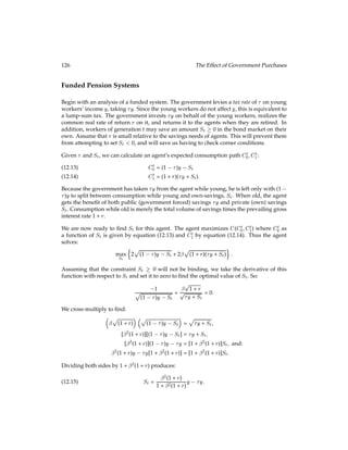
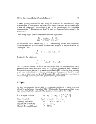
R = [ln($135K) ln($100K)](0:5) 0:15005230 = 15:15005230%:
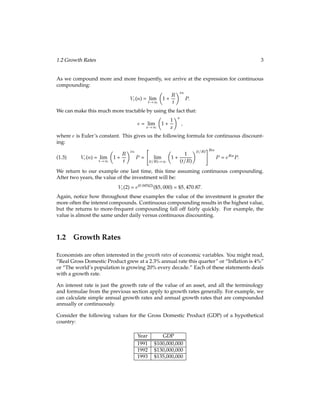
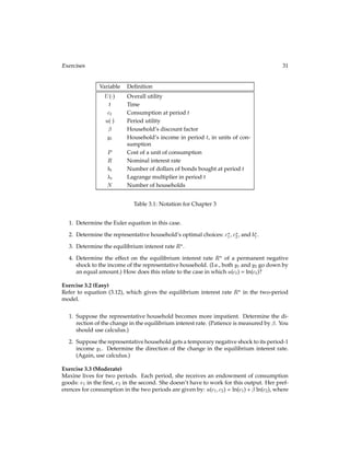
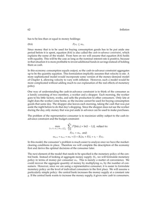
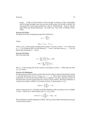
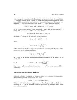
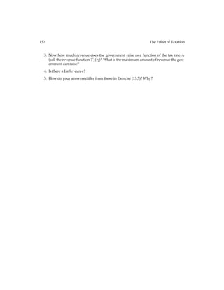
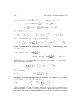
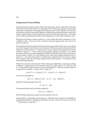
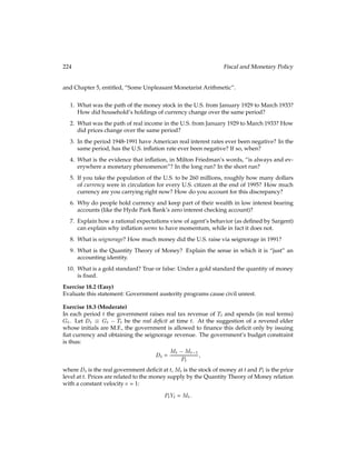
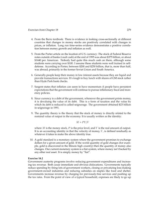
Economists generally prefer to use continuous compounding, for two reasons. First, un-
der continuous compounding, computing the growth rate between two values of a series
requires nothing more than taking the difference of their natural logarithms, as above.
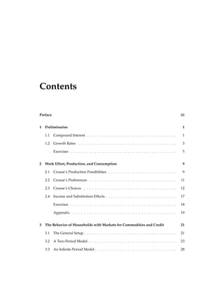
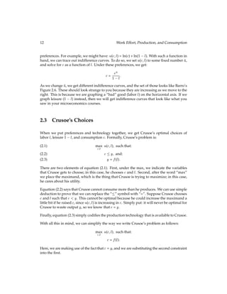
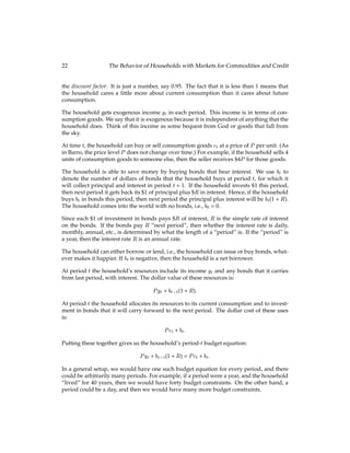
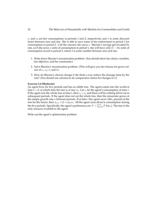
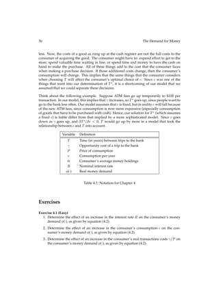
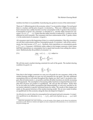
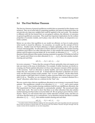
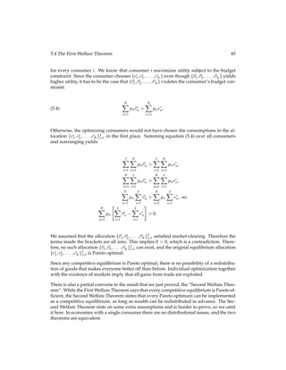
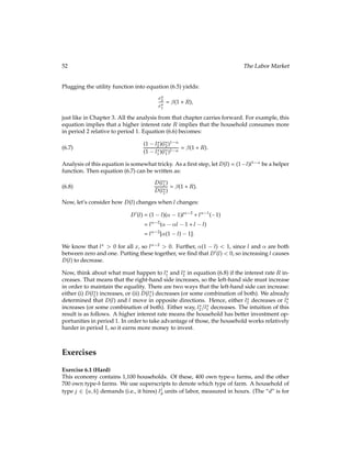
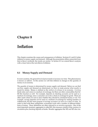
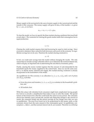
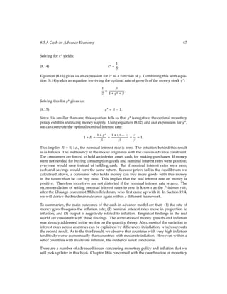
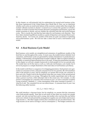
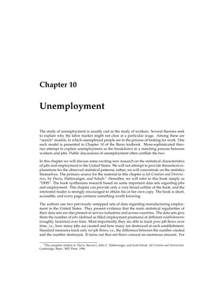
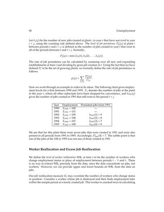
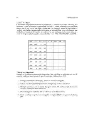
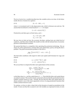
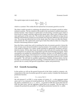
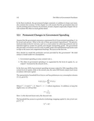
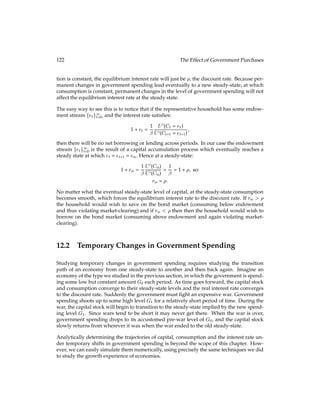
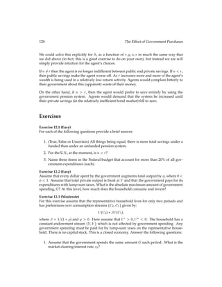
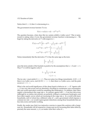
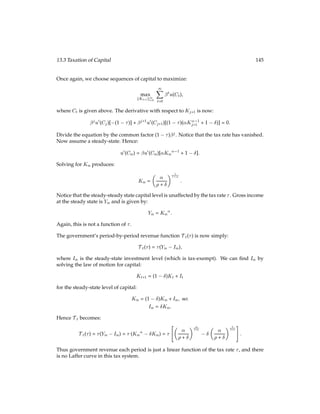
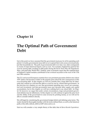
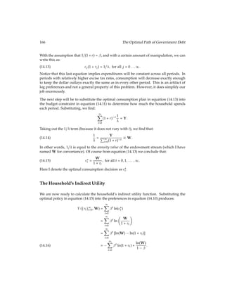
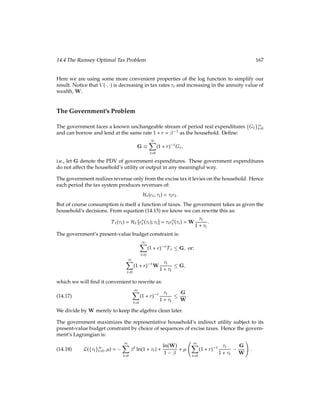
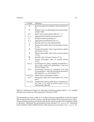
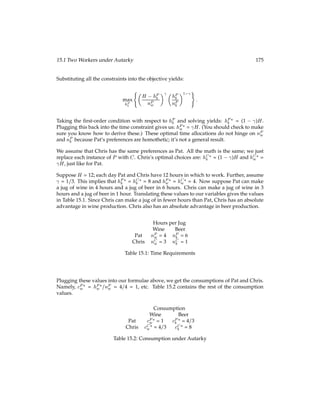
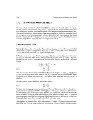
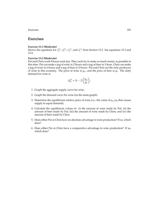
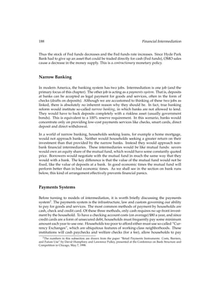
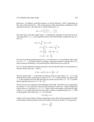
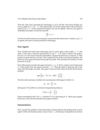
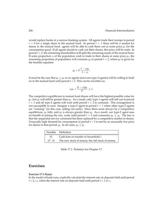
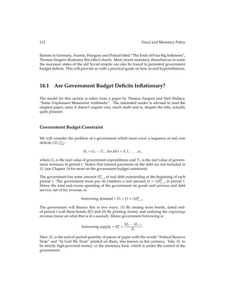
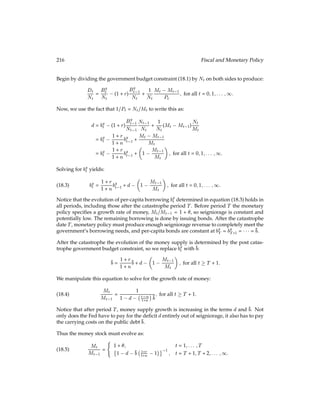
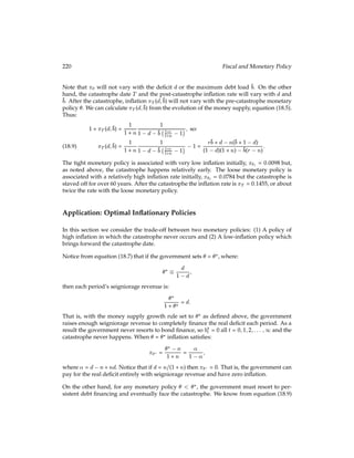
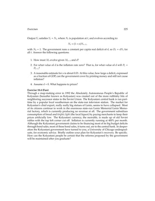
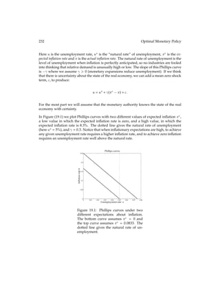
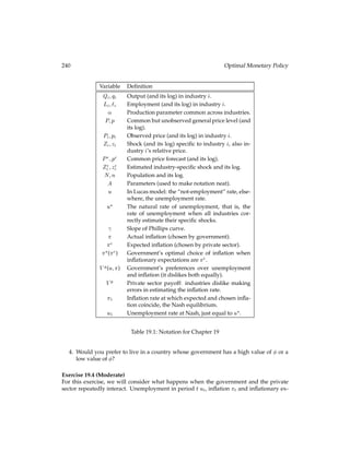
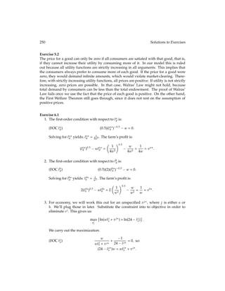
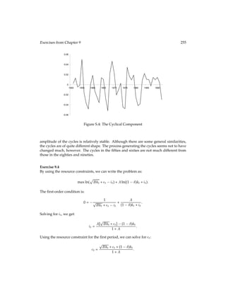
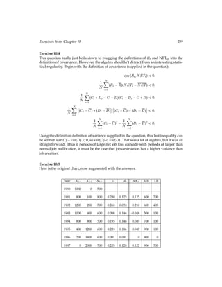
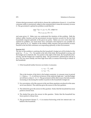
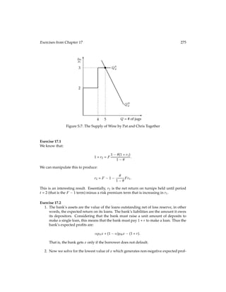
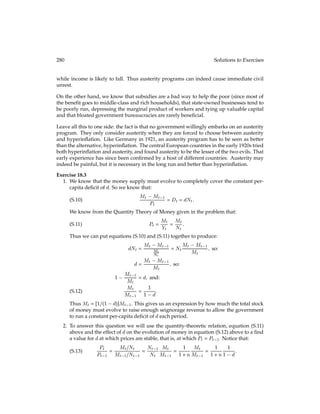
This property is useful when graphing series. For example, consider some series that is
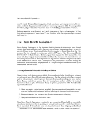
given by V(n) = V0e0:08n, which is depicted in Figure 1.1. By the equations above, we know
that this series grows at an 8% continuous rate. Figure 1.2 depicts the natural logarithm of
the same series, i.e., ln[V(n)] = ln(V0) + 0:08n. From the equation, you can see that this new
series is linear in n, and the slope (0.08) gives the growth rate. Whenever Barro labels the
vertical axis of a graph with “Proportionate scale”, he has graphed the natural logarithm
of the underlying series. For an example, see Barro’s Figure 1.1.
The second reason economists prefer continuous growth rates is that they have the follow-
ing desirable property: if you compute the year-by-year continuous growth rates of a series
and then take the average of those rates, the result is equal to the continuous growth rate
over the entire interval.
For example, consider the hypothetical GDP numbers from above: $100K, $130K, and
$135K. The continuous growth rate between the first two is: ln($130K) ln($100K). The
continuous growth rate between the second two is: ln($135K) ln($130K). The average of
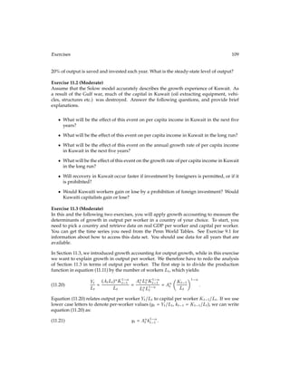
these two is:
ln($135K) ln($130K)
+
ln($130K) ln($100K)
2
:

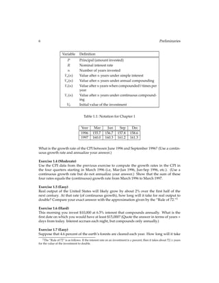
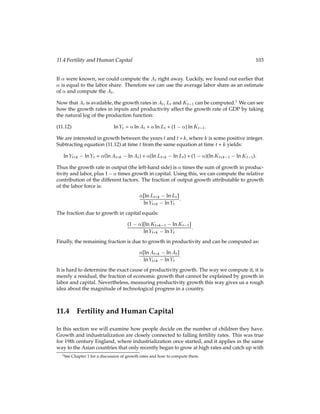
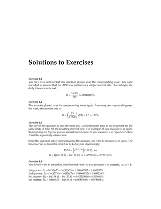
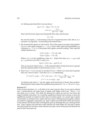
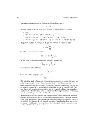
15. Exercises 5
0
2
4
6
8
0
5
10
15
20
25
Year (n)
V(n)
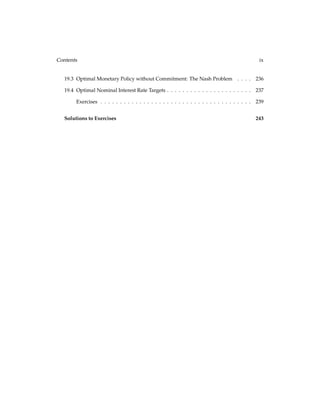
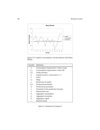
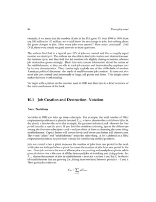
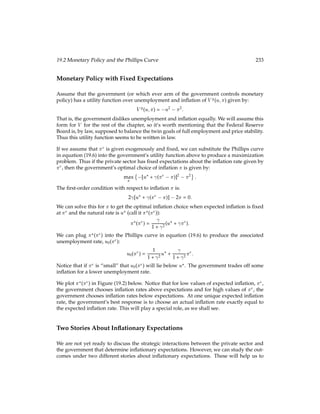
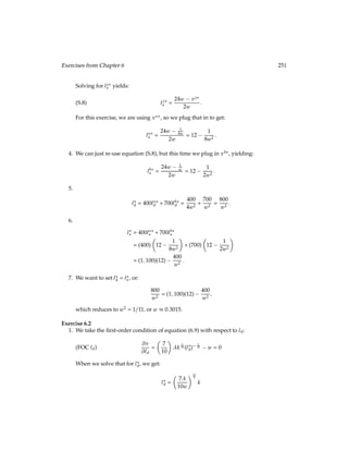
Figure 1.1: Exponential Growth
0
1
2
0
5
10
15
20
25
Year (n)
ln[V(n)]
Figure 1.2: Log of Exp Growth
The two ln($130K) terms cancel, leaving exactly the formula for the continuous growth
rate between the first and third values, as we derived above.
If we carry out the same exercise under simple growth or annually compounded growth,
we will find that the average of the individual growth rates will not equal the overall
growth rate. For example, if GDP grows by 8% this year and 4% next year, both calcu-
lated using annual compounding, then the two-year growth rate will not be 6%. (You
should verify that it will actually be 5.98%.) On the other hand, if the 8% and 4% numbers
were calculated using continuous compounding, then the continuous growth rate over the
two-year period would be 6%.
Exercises
Exercise 1.1 (Easy)
My credit card has an APR (annualized percentage rate) of 16.8%. What is the daily interest
rate?
Exercise 1.2 (Easy)
My loan shark is asking for $25 in interest for a one-week loan of $1,000. What is that, as
an annual interest rate? (Use 52 weeks per year.)
Exercise 1.3 (Moderate)
The Consumer Price Index (CPI) is a measure of the prices of goods that people buy. Bigger
numbers for the index mean that things are more expensive. Here are the CPI numbers for
four months of 1996 and 1997:

16. 6 Preliminaries
Variable Definition
P Principal (amount invested)
R Nominal interest rate
n Number of years invested
Vs(n) Value after n years under simple interest
Va(n) Value after n years under annual compounding
Vt(n) Value after nyears when compounded ttimes per
year
Vc(n) Value after nyears under continuous compound-
ing
V0 Initial value of the investment
Table 1.1: Notation for Chapter 1
Year Mar Jun Sep Dec
1996 155.7 156.7 157.8 158.6
1997 160.0 160.3 161.2 161.3
What is the growth rate of the CPI between June 1996 and September 1996? (Use a contin-
uous growth rate and annualize your answer.)
Exercise 1.4 (Moderate)
Use the CPI data from the previous exercise to compute the growth rates in the CPI in
the four quarters starting in March 1996 (i.e, Mar-Jun 1996, Jun-Sep 1996, etc.). (Use a
continuous growth rate but do not annualize your answer.) Show that the sum of these
four rates equals the (continuous) growth rate from March 1996 to March 1997.
Exercise 1.5 (Easy)
Real output of the United States will likely grow by about 2% over the first half of the
next century. At that rate (of continuous growth), how long will it take for real output to
double? Compare your exact answer with the approximation given by the “Rule of 72.”2
Exercise 1.6 (Hard)
This morning you invest $10,000 at 6.5% interest that compounds annually. What is the
first date on which you would have at least $15,000? (Quote the answer in terms of years +
days from today. Interest accrues each night, but compounds only annually.)
Exercise 1.7 (Easy)
Suppose that 4.6 percent of the earth’s forests are cleared each year. How long will it take
2The “Rule of 72” is as follows. If the interest rate on an investment is x percent, then it takes about 72=x years
for the value of the investment to double.

17. Exercises 7
for half our current forests to be cleared? (Use annual compounding and solve for the
fewest number of whole years.)
Exercise 1.8 (Moderate)
World population was about 679 million in the year 1700 and about 954 million in 1800.
1. What was the annual growth rate of population between 1700 and 1800? (Use con-
tinuous compounding.)
2. Suppose that the human race began with Adam and Eve and that the annual growth
rate between 1700 and 1800 prevailed in all years prior to 1700. About when must it
have been that Adam and Eve were evicted from the Garden of Eden? (Hint: What
was the population in that year?)
Exercise 1.9 (Moderate)
According to figures compiled by the World Bank, per capita real income in the U.S. was
$15,400 in 1984, while the corresponding figure for Japan was $10,600. Between 1965 and
1984, per capita real income in the U.S. grew at an annual rate of 1.7 percent (using annual
compounding), while the corresponding figure for Japan was 4.7 percent.
1. If these two growth rates remain constant at their 1965-84 levels, in what year will
per capita real income be the same in these two countries? (Again, use annual com-
pounding, and use hundredths of a year.)
2. What will be the common per capita real income of these two countries at that date?

19. Chapter 2
Work Effort, Production, and
Consumption
Robinson Crusoe is alone on an island, so he is an economy unto himself. He has prefer-
ences over consumption and leisure and can produce consumption goods by using labor
and capital. We examine production first. Then we turn to preferences. Putting these two
pieces together yields Crusoe’s optimal choices of labor, leisure, and consumption.
2.1 Crusoe’s Production Possibilities
Crusoe uses factors of production in order to make output y. We can think of this output as
being coconuts. Two common factors of production, and those we consider here, are capital
kand labor l. Capital might be coconut trees, and labor is the amount of time Crusoe works,
measured as a fraction of a day. How much Crusoe produces with given resources depends
on the type of technology A that he employs. We formalize this production process via a
production function.
We often simplify our problems by assuming that the production function takes some par-
ticular functional form. As a first step, we often assume that it can be written: y = Af(k;l),
for some function f(). This means that as technology A increases, Crusoe can get more
output for any given inputs. It is reasonable to require the function f() to be increasing
in each argument. This implies that increasing either input k or l will increase production.
Another common assumption is that output is zero if either input is zero: f(0;l) = 0 and
f(k;0) = 0, for all k and l.
One functional form that has these properties is the Cobb–Douglas function, for example:

20. 10 Work Effort, Production, and Consumption
y = Ak1 l, for some between zero and one. This particular Cobb-Douglas function
exhibits constant returns to scale, since (1 ) + () = 1. Figure 2.1 is a three-dimensional
rendering of this function for particular values of A and .
0
0.2
0.4
0.6
0.8
1
0
0.2
0.4
0.6
0.8
1
0
0.2
0.4
0.6
0.8
1
product
(y)
labor (l)
capital (k)
Figure 2.1: Cobb-Douglas Production
We will not be dealing with capital k until Chapter 9, so for now we assume that capital is
fixed, say, at k = 1. This simplifies the production function. With a slight abuse of notation,
we redefine f() and write production as y = f(l). This is like what Barro uses in Chapter 2.
If the original production function was Cobb–Douglas, y = Ak1 l, then under k = 1 the
production function becomes: y = Al. The graph of this curve is just a slice through the
surface depicted in Figure 2.1. It looks like Barro’s Figure 2.1.
As you know, the marginal product of some factor of production (e.g., labor l) is the addi-
tional output, or “product”, that results from increasing the input of that factor. Formally,
the marginal product of an input is the derivative of the production function with respect to

21. 2.2 Crusoe’s Preferences 11
that input. For example, the marginal product of labor is: dy=dl = f0(l).1
Since the marginal
product is the derivative of the the production function, and the derivative gives the slope,
we can read the marginal product as the slope of the production function, as Barro does in
his Figure 2.1.
In the particular case where production is Cobb–Douglas (and capital is fixed), the produc-
tion function is: y = Al, so the marginal product of labor is: dy=dl = Al 1
. This is always
positive, as we require, and it decreases as we increase l. Accordingly, this production func-
tion exhibits diminishing marginal product: the first unit of labor is more productive than
the tenth unit of labor. Graphing this marginal product equation gives us something like
Barro’s Figure 2.2.
Barro talks about improvements in technology and argues how both the production func-
tion and the marginal-product schedule shift as a result. The effects of such a change in
technology are clearer when we examine a particular production function. For example,
consider our production function: y = Al. The improvement in technology means that A
goes up. Accordingly, whatever production was before, it undergoes the same percentage
increase as the increase in A. For example, if A doubles, then output at each l will be dou-
ble what it used to be. Notably, when l is zero, output is zero just as before, since twice
zero is still zero. The result is that the production function undergoes a kind of upward
rotation, pivoting about the anchored origin, l = 0. That is precisely what Barro depicts in
his Figure 2.3.
We can examine the marginal-product schedule as well. Under the particular functional
form we are using, the marginal product of labor (MPL) is: dy=dl = Al 1
. Accordingly,
the marginal product at each l undergoes the same percentage change as does A. Since the
MPL is higher at low levels of l, the marginal-product curve shifts up more at those levels
of l. Refer to Barro’s Figure 2.4.
2.2 Crusoe’s Preferences
Crusoe cares about his consumption cand his leisure. Since we are measuring labor las the
fraction of the day that Crusoe works, the remainder is leisure. Specifically, leisure is 1 l.
We represent his preferences with a utility function u(c;l). Take note, the second argument
is not a “good” good, since Crusoe does not enjoy working. Accordingly, it might have
been less confusing if Barro had written utility as v(c;1 l), for some utility function v().
We assume that Crusoe’s preferences satisfy standard properties: they are increasing in
each “good” good, they are convex, etc.
We will often simplify the analysis by assuming a particular functional form for Crusoe’s
1Barro uses primes to denote shifted curves rather than derivatives. For example, when Barro shifts the f(l)
curve, he labels the new curve f(l)0. This is not a derivative. Barro’s notation is unfortunate, but we are stuck
with it.

22. 12 Work Effort, Production, and Consumption
preferences. For example, we might have: u(c;l) = ln(c) + ln(1 l). With such a function in
hand, we can trace out indifference curves. To do so, we set u(c;l) to some fixed number ū,
and solve for c as a function of l. Under these preferences, we get:
c =
eū
1 l:
As we change ū, we get different indifference curves, and the set of those looks like Barro’s
Figure 2.6. These should look strange to you because they are increasing as we move to the
right. This is because we are graphing a “bad” good (labor l) on the horizontal axis. If we
graph leisure (1 l) instead, then we will get indifference curves that look like what you
saw in your microeconomics courses.
2.3 Crusoe’s Choices
When we put preferences and technology together, we get Crusoe’s optimal choices of
labor l, leisure 1 l, and consumption c. Formally, Crusoe’s problem is:
max
c;l
u(c;l); such that:
(2.1)
c y; and:
(2.2)
y = f(l):
(2.3)
There are two elements of equation (2.1). First, under the max, we indicate the variables
that Crusoe gets to choose; in this case, he chooses c and l. Second, after the word “max”
we place the maximand, which is the thing that Crusoe is trying to maximize; in this case,
he cares about his utility.
Equation (2.2) says that Crusoe cannot consume more than he produces. We can use simple
deduction to prove that we can replace the “” symbol with “=”. Suppose Crusoe chooses
c and l such that c y. This cannot be optimal because he could increase the maximand a
little bit if he raised c, since u(c;l) is increasing in c. Simply put: it will never be optimal for
Crusoe to waste output y, so we know that c = y.
Finally, equation (2.3) simply codifies the production technology that is available to Crusoe.
With all this in mind, we can simplify the way we write Crusoe’s problem as follows:
max
c;l
u(c;l); such that:
c = f(l):
Here, we are making use of the fact that c = y, and we are substituting the second constraint
into the first.

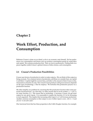
23. 2.3 Crusoe’s Choices 13
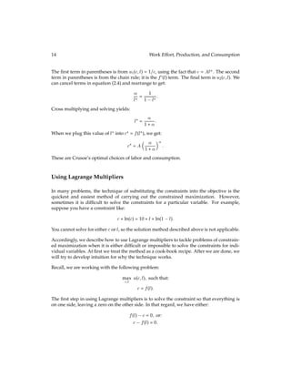
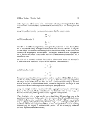
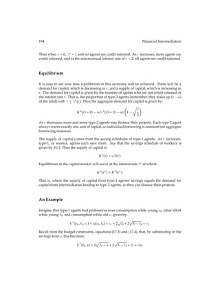
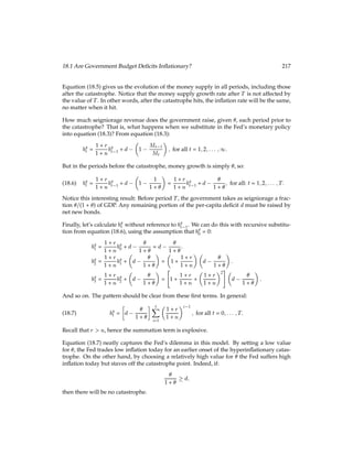
There are two principal ways to solve such a problem. The first is to substitute any con-
straints into the objective. The second is to use Lagrange multipliers. We consider these
two methods in turn.
Substituting Constraints into the Objective
In the maximization problem we are considering, we have c in the objective, but we know
that c = f(l), so we can write the max problem as:
max
l
u[f(l);l]:
We no longer have c in the maximand or in the constraints, so c is no longer a choice
variable. Essentially, the c = f(l) constraint tacks down c, so it is not a free choice. We
exploit that fact when we substitute c out.
At this point, we have a problem of maximizing some function with respect to one vari-
able, and we have no remaining constraints. To obtain the optimal choices, we take the
derivative with respect to each choice variable, in this case l alone, and set that derivative
equal to zero.2
When we take a derivative and set it equal to zero, we call the resulting
equation a first-order condition, which we often abbreviate as “FOC”.
In our example, we get only one first-order condition:
d
dl fu[f(l?);l?]g = u1[f(l?);l?]f0(l?) + u2[f(l?);l?] = 0:
(FOC l)
(See the Appendix for an explanation of the notation for calculus, and note how we had to
use the chain rule for the first part.) We use l? because the l that satisfies this equation will
be Crusoe’s optimal choice of labor.3
We can then plug that choice back into c = f(l) to get
Crusoe’s optimal consumption: c? = f(l?). Obviously, his optimal choice of leisure will be
1 l?.
Under the particular functional forms for utility and consumption that we have been con-
sidering, we can get explicit answers for Crusoe’s optimal choices. Recall, we have been
using u(c;l) = ln(c) + ln(1 l) and y = f(l) = Al. When we plug these functions into the
first-order condition in equation (FOC l), we get:
1
A(l?)
A(l?) 1
+
1
1 l? = 0:
(2.4)
2The reason we set the derivative equal to zero is as follows. The maximand is some hump-shaped object. The
derivative of the maximand gives the slope of that hump at each point. At the top of the hump, the slope will be
zero, so we are solving for the point at which the slope is zero.
3Strictly speaking, we also need to check the second-order condition in order to make sure that we have
solved for a maximum instead of a minimum. In this text we will ignore second-order conditions because they
will always be satisfied in the sorts of problems we will be doing.

24. 14 Work Effort, Production, and Consumption
The first term in parentheses is from u1(c;l) = 1=c, using the fact that c = Al. The second
term in parentheses is from the chain rule; it is the f0(l) term. The final term is u2(c;l). We
can cancel terms in equation (2.4) and rearrange to get:
l? =
1
1 l? :
Cross multiplying and solving yields:
l? =
1 + :
When we plug this value of l? into c? = f(l?), we get:
c? = A
1 +
:
These are Crusoe’s optimal choices of labor and consumption.
Using Lagrange Multipliers
In many problems, the technique of substituting the constraints into the objective is the
quickest and easiest method of carrying out the constrained maximization. However,
sometimes it is difficult to solve the constraints for a particular variable. For example,
suppose you have a constraint like:
c+ ln(c) = 10 + l+ ln(1 l):
You cannot solve for either cor l, so the solution method described above is not applicable.
Accordingly, we describe how to use Lagrange multipliers to tackle problems of constrain-
ed maximization when it is either difficult or impossible to solve the constraints for indi-
vidual variables. At first we treat the method as a cook-book recipe. After we are done, we
will try to develop intuition for why the technique works.
Recall, we are working with the following problem:
max
c;l
u(c;l); such that:
c = f(l):
The first step in using Lagrange multipliers is to solve the constraint so that everything is
on one side, leaving a zero on the other side. In that regard, we have either:
f(l) c = 0; or:
c f(l) = 0:

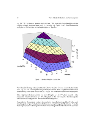
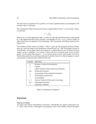
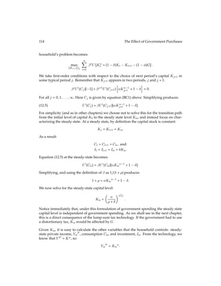
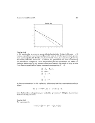
25. 2.3 Crusoe’s Choices 15
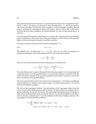
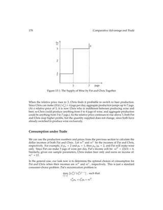
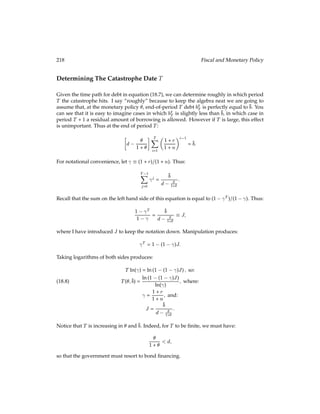
Either of those two will work, but we want to choose the first one, for reasons that are
described below. The general heuristic is to choose the one that has a minus sign in front
of the variable that makes the maximand larger. In this case, more c makes utility higher,
so we want the equation with c.
The second step is to write down a function called the Lagrangean, defined as follows:
L(c;l;) = u(c;l) + [f(l) c]:
As you can see, the Lagrangean is defined to be the original objective, u(c;l), plus some
variable times our constraint. The Lagrangean is a function; in this case its arguments
are the three variables c, l, and . Sometimes we will write it simply as L, suppressing
the arguments. The variable is called the Lagrange multiplier; it is just some number that
we will calculate. If there is more than one constraint, then each one is: (i) solved for
zero; (ii) multiplied by its own Lagrange multiplier, e.g., 1, 2, etc.; and (iii) added to the
Lagrangean. (See Chapter 3 for an example.)
Before we used calculus to maximize our objective directly. Now, we work instead with
the Lagrangean. The standard approach is to set to zero the derivatives of the Lagrangian
with respect to the choice variables and the Lagrange multiplier . The relevant first-order
conditions are:
@
@c [L(c?;l?;?)] = u1(c?;l?) + ?[ 1] = 0;
(FOC c)
@
@l [L(c?;l?;?)] = u2(c?;l?) + ?[f0(l?)] = 0; and:
(FOC l)
@
@ [L(c?;l?;?)] = f(l?) c? = 0:
(FOC )
Again, we use starred variables in these first-order conditions to denote that it is only for
the optimal values of c, l, and that these derivatives will be zero. Notice that differen-
tiating the Lagrangian with respect to simply gives us back our budget equation. Now
we have three equations in three unknowns (c?, l?, and ?) and can solve for a solution.
Typically, the first step is to use equations (FOC c) and (FOC l) to eliminate ?. From (FOC
c) we have:
u1(c?;l?) = ?;
and from (FOC l) we have:
u2(c?;l?)
f0(l?)
= ?:
Combining the two gives us:
u1(c?;l?) =
u2(c?;l?)
f0(l?)
:
(2.5)

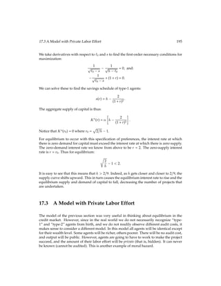
26. 16 Work Effort, Production, and Consumption
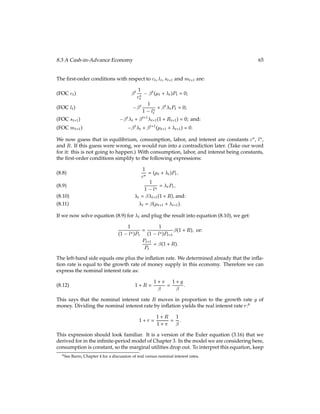
When we are given particular functional forms for u() and f(), then equation (2.5) gives
us a relationship between c? and l? that we can plug into the budget equation and solve
further. For example, under u(c;l) = ln(c) + ln(1 l) and f(l) = Al, equation (2.5) becomes:
1
c? =
1
1 l?
1
A(l?) 1
;
or equivalently:
c? = A(1 l?)(l?) 1
:
Now we plug in the budget equation c = Al to get:
A(l?) = A(1 l?)(l?) 1
:
After some canceling and algebraic manipulation, this reduces to:
l? =
1 + :
Finally, we plug this answer for the optimal labor l? back into the budget equation to get:
c? = A
1 +
:
Notice that these are the same answers for c? and l? that we derived in the previous sub-
section, when we plugged the constraint into the objective instead of using a Lagrange
multiplier.
Now let’s try to figure out why the technique of Lagrange multipliers works. First, we
want to understand better what the Lagrange multiplier is. Our first-order condition
with respect to c gave us:
u1(c?;l?) = ?;
(2.6)
This tells us that, at the optimum, ? is the marginal utility of an extra unit of consumption,
given by the left-hand side. It is this interpretation of that motivated our choice of f(l)
c = 0 rather than c f(l) = 0 when we attached the constraint term to the Lagrangean. If
we had used the latter version of the constraint, then the right-hand side of equation (2.6)
would have been , which would have been minus the marginal utility of income.
Now look at the terms in the Lagrangian:
L(c;l;) = u(c;l) + [f(l) c]:
It contains our objective u() and then the Lagrange multiplier times the constraint. Re-
member, is the marginal utility of an additional unit of consumption. Notice that if the
budget equation is satisfied, then f(l) = c, so the constraint term is zero, and the Lagrangian
Land the objective u() are equal. Ceteris paribus, the Lagrangian will be big whenever the
objective is.

27. 2.4 Income and Substitution Effects 17
Now, think about the contributions from the constraint term. Suppose Crusoe is at some
choice of c and l such that the budget is exactly met. If he wants to decrease labor l by a
little bit, then he will have to cut back on his consumption c. The constraint term in the
Lagrangean is: [f(l) c]. The Lagrangean, our new objective, goes down by the required
cut in c times , which is the marginal utility of consumption. Essentially, the Lagrangean
subtracts off the utility cost of reducing consumption to make up for shortfalls in budget
balance. That way, the Lagrangean is an objective that incorporates costs from failing to
meet the constraint.
2.4 Income and Substitution Effects
Barro uses graphs to examine how Crusoe’s optimal choices of consumption and labor
change when his production function shifts and rotates. He calls the changes in Crusoe’s
choices “wealth and substitution effects”. That discussion is vaguely reminiscent of your
study of income and substitution effects from microeconomics. In that context, you con-
sidered shifts and rotations of linear budget lines. Crusoe’s “budget line” is his production
function, which is not linear.
This difference turns out to make mathematical calculation of income and substitution ef-
fects impractical. Furthermore, the “wealth effects” that Barro considers violate our as-
sumption that production is zero when labor l is zero. Such a wealth effect is depicted
as an upward shift of the production function in Barro’s Figure 2.8. This corresponds to
adding a constant to Crusoe’s production function, which means that production is not
zero when l is.
Barro’s Figure 2.10 depicts a pivot of the production about the origin. This type of change
to production is much more common in macroeconomics, since it is how we typically rep-
resent technological improvements. If Crusoe’s production function is y = Al, then an
increase in A will look exactly like this. Given a specific functional form for u() as well, it
is straightforward to compute how Crusoe’s choices of consumption c and labor l change
for any given change in A.
For example, suppose u(c;l) = ln(c) + ln(1 l) as before. Above we showed that:
c? = A
1 +
:
Determining how c? changes when A changes is called comparative statics. The typical
exercise is to take the equation giving the optimal choice and to differentiate it with respect
to the variable that is to change. In this case, we have an equation for Crusoe’s optimal
choice of c?, and we are interested in how that choice will change as A changes. That gives
us:
@c?
@A =
1 +
:
(2.7)

28. 18 Work Effort, Production, and Consumption
The derivative in equation (2.7) is positive, so Crusoe’s optimal choice of consumption will
increase when A increases.
The comparative statics exercise for Crusoe’s optimal labor choice l? is even easier. Above
we derived:
l? =
1 + :
There is no A on the right-hand side, so when we take the partial derivative with respect
to A, the right-hand side is just a constant. Accordingly, @l?=@A = 0, i.e., Crusoe’s choice of
labor effort does not depend on his technology. This is precisely what Barro depicts in his
Figure 2.10.
The intuition of this result is as follows. When A goes up, the marginal product of labor
goes up, since the slope of the production function goes up. This encourages Crusoe to
work harder. On the other hand, the increase in A means that for any l Crusoe has more
output, so he is wealthier. As a result, Crusoe will try to consume more of any normal
goods. To the extent that leisure 1 l is a normal good, Crusoe will actually work less.
Under these preferences and this production function, these two effects happen to cancel
out precisely. In general, this will not be the case.
Variable Definition
y Income, in units of consumption
k Capital
l Labor, fraction of time spent on production
f(l) Production function
A parameter of the production function
A Technology of production
c Consumption
1 l Leisure, fraction of time spent recreating
L() Lagrangean function
Lagrange multiplier
Table 2.1: Notation for Chapter 2
Exercises
Exercise 2.1 (Easy)
An agent cares about consumption and leisure. Specifically, the agent’s preferences are:
U = ln(c)+ln(l), where cis the agent’s consumption, and l is the number of hours the agent

29. Appendix: Calculus Notation 19
spends per day on leisure. When the agent isn’t enjoying leisure time, the agent works,
either for herself or for someone else. If she works ns hours for herself, then she produces
y = 4n0:5
s units of consumption. For each hour that she works for someone else, she gets
paid a competitive wage w, in units of consumption.
Write out the agent’s optimization problem.
Exercise 2.2 (Moderate)
Suppose Crusoe’s preferences are given by: u(c;l) = c
(1 l)1
, for some
between zero
and one. His technology is: y = f(l) = Al, just like before. Solve for Crusoe’s optimal
choices of consumption cand labor l. (You can use either substitution or a Lagrangean, but
the former is easier in this sort of problem.)
Appendix: Calculus Notation
Suppose we have a function: y = f(x). We can think of differentiation as an operator that
acts on objects. Write d
dx as the operator that differentiates with respect to x. We can apply
the operator to both sides of any equation. Namely,
d
dx y
=
d
dx f(x)
:
We often write the left-hand side as dy
dx, and the right-hand side as f0(x). These are just
notational conventions.
When we have functions of more than one variable, we are in the realm of multivariate
calculus and require more notation. Suppose we have z = f(x;y). When we differenti-
ate such a function, we will take partial derivatives that tell us the change in the function
from changing only one of the arguments, while holding any other arguments fixed. Par-
tial derivatives are denoted with curly dees (i.e., with @) to distinguish them from normal
derivatives. We can think of partial differentiation as an operator as before:
@
@x z
=
@
@x f(x;y)
:
The left-hand side is often written as @z
@x, and the right-hand side as f1(x;y). The subscript
1 on f indicates a partial derivative with respect to the first argument of f. The derivative
of f with respect to its second argument, y, can similarly be written: f2(x;y).
The things to remember about this are:
Primes (f0) and straight dees (df) are for functions of only one variable.
Subscripts (f1) and curly dees (@f) are for functions of more than one variable.

31. Chapter 3
The Behavior of Households with
Markets for Commodities and
Credit
In this chapter we move from the world in which Robinson Crusoe is alone on his island
to a world of many identical households that interact. To begin, we consider one particular
representative household. When we add together the behaviors of many households, we
get a macroeconomy.
Whereas in Chapter 2 we looked at Crusoe’s choices between consumption and leisure
at one point in time, now we consider households’ choices of consumption over multiple
periods, abstracting from the labor decisions of households. Section 3.1 introduces the
basic setup of the chapter. In Section 3.2 we work out a model in which households live for
only two periods. Households live indefinitely in the model presented in Section 3.3. Both
these models follow Barro fairly closely, but of course in greater mathematical detail. The
primary difference is that Barro has households carry around money, while we do not.
3.1 The General Setup
The representative household cares about consumption ct in each period. This is formal-
ized by some utility function U(c1;c2;c3;:::). Economists almost always simplify intertem-
poral problems by assuming that preferences are additively separable. Such preferences
look like: U(c1;c2;c3;:::) = u(c1) +

32. u(c2) +

33. 2
u(c3) + . The u() function is called the
period utility. It satisfies standard properties of utility functions. The variable

34. is called

35. 22 The Behavior of Households with Markets for Commodities and Credit
the discount factor. It is just a number, say 0.95. The fact that it is less than 1 means that
the household cares a little more about current consumption than it cares about future
consumption.
The household gets exogenous income yt in each period. This income is in terms of con-
sumption goods. We say that it is exogenous because it is independent of anything that the
household does. Think of this income as some bequest from God or goods that fall from
the sky.
At time t, the household can buy or sell consumption goods ct at a price of P per unit. (As
in Barro, the price level P does not change over time.) For example, if the household sells 4
units of consumption goods to someone else, then the seller receives $4P for those goods.
The household is able to save money by buying bonds that bear interest. We use bt to
denote the number of dollars of bonds that the household buys at period t, for which it
will collect principal and interest in period t + 1. If the household invests $1 this period,
then next period it gets back its $1 of principal plus $R in interest. Hence, if the household
buys bt in bonds this period, then next period the principal plus interest will be bt(1 + R).
The household comes into the world with no bonds, i.e., b0 = 0.
Since each $1 of investment in bonds pays $R of interest, R is the simple rate of interest
on the bonds. If the bonds pay R “next period”, then whether the interest rate is daily,
monthly, annual, etc., is determined by what the length of a “period” is. If the “period” is
a year, then the interest rate R is an annual rate.
The household can either borrow or lend, i.e., the household can issue or buy bonds, what-
ever makes it happier. If bt is negative, then the household is a net borrower.
At period t the household’s resources include its income yt and any bonds that it carries
from last period, with interest. The dollar value of these resources is:
Pyt + bt 1(1 + R):
At period t the household allocates its resources to its current consumption and to invest-
ment in bonds that it will carry forward to the next period. The dollar cost of these uses
is:
Pct + bt:
Putting these together gives us the household’s period-tbudget equation:
Pyt + bt 1(1 + R) = Pct + bt:
In a general setup, we would have one such budget equation for every period, and there
could be arbitrarily many periods. For example, if a period were a year, and the household
“lived” for 40 years, then we would have forty budget constraints. On the other hand, a
period could be a day, and then we would have many more budget constraints.

36. 3.2 A Two-Period Model 23
3.2 A Two-Period Model
We begin this section with a discussion of the choices of a representative household. Then
we put a bunch of these households together and discuss the resulting macroeconomic
equilibrium.
Choices of the Representative Household
In this model the household lives for two time periods, t = 1;2. In this case, the household’s
preferences reduce to:
U(c1;c2) = u(c1) +

37. u(c2):
(3.1)
Given that the household will not be around to enjoy consumption in period 3, we know
that it will not be optimal for the household to buy any bonds in period 2, since those bonds
would take away from period-2 consumption c2 and provide income only in period 3, at
which time the household will no longer be around. Accordingly, b2 = 0. That leaves only
b1 in this model.
The household’s budget constraints simplify as well. In period 1 the household’s budget
equation is:
Py1 = Pc1 + b1;
(3.2)
and in period t = 2 it is:
Py2 + b1(1 + R) = Pc2:
(3.3)
The household’s problem is to choose consumptions c1 and c2 and first-period bond hold-
ings b1 so as to maximize utility (3.1) subject to the budget equations (3.2) and (3.3). The
household takes the price level P and the interest rate R as given.
We write out the household’s problem:
max
c1;c2;b1
fu(c1) +

38. u(c2)g; subject to:
(3.4)
Py1 = Pc1 + b1; and:
(3.5)
Py2 + b1(1 + R) = Pc2:
(3.6)
We solve this problem by using the method of Lagrange multipliers. The Lagrangean is:
L = u(c1) +

39. u(c2) + 1[Py1 Pc1 b1] + 2[Py2 + b1(1 + R) Pc2];
where 1 and 2 are our two Lagrange multipliers. The first-order conditions are:
u0(c?
1 ) + ?
1 [ P] = 0;
(FOC c1)

40. u0(c?
2) + ?
2 [ P] = 0; and:
(FOC c2)
?
1 [ 1] + ?
2 [(1 + R)] = 0:
(FOC b1)

41. 24 The Behavior of Households with Markets for Commodities and Credit
(Again, stars denote that only the optimal choices will satisfy these first-order conditions.)
We leave off the first-order conditions with respect to the Lagrange multipliers 1 and 2,
since we know that they will give us back the two budget constraints.
Rewriting the first two FOCs gives us:
u0(c?
1 )
P = ?
1 ; and:

42. u0(c?
2 )
P = ?
2 :
We can plug these into the FOC with respect to b1 to get:
u0(c?
1 )
P +

43. u0(c?
2 )
P (1 + R) = 0;
which we can rewrite as:
u0(c?
1 )
u0(c?
2 )
=

44. (1 + R):
(3.7)
Equation (3.7) is called an Euler equation (pronounced: OIL-er). It relates the marginal
utility of consumption in the two periods. Given a functional form for u(), we can use this
equation and the two budget equations to solve for the household’s choices c?
1 , c?
2 , and b?
1 .
It is possible to use the Euler equation to make deductions about these choices even without
knowing the particular functional form of the period utility function u(), but this analysis is
much more tractable when the form of u() is given. Accordingly, we assume u(ct) = ln(ct).
Then u0(ct) = 1=ct, and equation (3.7) becomes:
c?
2
c?
1
=

45. (1 + R):
(3.8)
Before we solve for c?
1 , c?
2 , and b?
1 , let us think about this equation. Recall, preferences are:
u(c1)+

46. u(c2). Intuitively, if

47. goes up, then the household cares more about the future than
it used to, so we expect the household to consume more c2 and less c1.
This is borne out graphically in Barro’s Figure 3.4. Larger

48. corresponds to smaller slopes
in the household’s indifference curves, which rotate downward, counter-clockwise. Ac-
cordingly, the household’s choice of c2 will go up and that of c1 will go down, like we
expect.
We can show the result mathematically as well. An increase in

49. causes an increase in
right-hand side of the Euler equation (3.8), so c?
2 goes up relative to c?
1 , just like we expect.
Now we consider changes on the budget side. Suppose R goes up. Then the opportunity
cost of consumption c1 in the first period goes up, since the household can forego c1 and
earn a higher return on investing in bonds. By the same reasoning, the opportunity cost
of c2 goes down, since the household can forego less c1 to get a given amount of c2. Ac-
cordingly, if R goes up, we expect the household to substitute away from c1 and toward
c2.

50. 3.2 A Two-Period Model 25
Refer to Barro’s Figure 3.4. If R goes up, then the budget line rotates clockwise, i.e., it gets
steeper. This indicates that the household chooses larger c2 and smaller c1 (subject to being
on any given indifference curve), just like our intuition suggests.
Mathematically, we refer once again to the Euler equation. If Rgoes up, then the right-hand
side is larger, so c?
2 =c?
1 goes up, again confirming our intuition.
Given u(ct) = ln(ct), we can actually solve for the household’s optimal choices. The Euler
equation and equations (3.2) and (3.3) give us three equations in the three unknowns, c?
1 ,
c?
2 , and b?
1 . Solving yields:
c?
1 =
y2 + y1(1 + R)
(1 +

51. )(1 + R)
;
c?
2 =
y2 + y1(1 + R)

52. 1 +

53. ; and:
b?
1 = Py1
P[y2 + y1(1 + R)]
(1 +

54. )(1 + R)
:
You can verify these if you like. Doing so is nothing more than an exercise in algebra.
If we tell the household what the interest rate R is, the household performs its own maxi-
mization to get its choices of c1, c2, and b1, as above. We can write these choices as functions
of R, i.e., c?
1 (R), c?
2 (R), and b?
1(R), and we can ask what happens to these choices as the in-
terest rate R changes. Again, this exercise is called “comparative statics”. All we do is take
the derivative of the choices with respect to R. For example:
@c?
2
@R =
y1

55. 1 +

56. 0;
so c?
2 goes up as the interest rate goes up, like our intuition suggests.
Market Equilibrium
So far we have restricted attention to one household. A macroeconomy would be com-
posed of a number of these households, say N of them, so we stick these households to-
gether and consider what happens. In this model, that turns out to be trivial, since all
households are identical, but the exercise will give you practice for more-difficult settings
to come.
The basic exercise is to close our model by having the interest rate R determined endoge-
nously. Recall, we said that households can be either lenders or borrowers, depending on
whether b1 is positive or negative, respectively. Well, the only borrowers and lenders in
this economy are the N households, and all of them are alike. If they all want to borrow,
there will be no one willing to lend, and there will be an excess demand for loans. On the

57. 26 The Behavior of Households with Markets for Commodities and Credit
other hand, if they all want to lend, there will be an excess supply of loans. More formally,
we can write the aggregate demand for bonds as: Nb?
1 . Market clearing requires:
Nb?
1 = 0:
(3.9)
Of course, you can see that this requires that each household neither borrows nor lends,
since all households are alike.
Now we turn to a formal definition of equilibrium. In general, a competitive equilibrium is a
solution for all the variables of the economy such that: (i) all economic actors take prices as
given; (ii) subject to those prices, all economic actors behave rationally; and (iii) all markets
clear. When asked to define a competitive equilibrium for a specific economy, your task is
to translate these three conditions into the specifics of the problem.
For the economy we are considering here, there are two kinds of prices: the price of con-
sumption P and the price of borrowing R. The actors in the economy are the N households.
There are two markets that must clear. First, in the goods market, we have:
Nyt = Nc?
t ; t = 1;2:
(3.10)
Second, the bond market must clear, as given in equation (3.9) above. With all this written
down, we now turn to defining a competitive equilibrium for this economy.
A competitive equilibrium in this setting is: a price of consumption P?; an interest rate R?;
and values for c?
1 , c?
2 , and b?
1 , such that:
Taking P? and R? as given, all N households choose c?
1 , c?
2 , and b?
1 according to the
maximization problem given in equations (3.4)-(3.6);
Given these choices of c?
t , the goods market clears in each period, as given in equa-
tion (3.10); and
Given these choices of b?
1, the bond market clears, as given in equation (3.9).
Economists are often pedantic about all the detail in their definitions of competitive equi-
libria, but providing the detail makes it very clear how the economy operates.
We now turn to computing the competitive equilibrium, starting with the credit market.
Recall, we can write b?
1 as a function of the interest rate R, since the lending decision of
each household hinges on the interest rate. We are interested in finding the interest rate
that clears the bond market, i.e., the R? such that b?
1 (R?) = 0. We had:
b?
1 (R) = Py1
P[y2 + y1(1 + R)]
(1 +

58. )(1 + R)
;
so we set the left-hand side to zero and solve for R?:
Py1 =
P[y2 + y1(1 + R?)]
(1 +

59. )(1 + R?)
:
(3.11)

60. 3.2 A Two-Period Model 27
After some algebra, we get:
R? =
y2

61. y1
1:
(3.12)
This equation makes clear that the equilibrium interest rate is determined by the incomes
(y1 and y2) of the households in each period and by how impatient the households are (

62. ).
We can perform comparative statics here just like anywhere else. For example:
@R?
@y2
=
1

63. y1
0;
so if second-period income increases, then R? does too. Conversely, if second-period in-
come decreases, then R? does too. This makes intuitive sense. If y2 goes down, households
will try to invest first-period income in bonds in order to smooth consumption between
the two periods. In equilibrium this cannot happen, since net bond holdings must be zero,
so the equilibrium interest rate must fall in order to provide a disincentive to investment,
exactly counteracting households’ desire to smooth consumption.
You can work through similar comparative statics and intuition to examine how the equi-
librium interest rate changes in response to changes in y1 and

64. . (See Exercise 3.2.)
Take note that in this model and with these preferences, only relative incomes matter. For
example, if both y1 and y2 shrink by 50%, then y2=y1 does not change, so the equilibrium
interest rate does not change. This has testable implications. Namely, we can test the
reaction to a temporary versus a permanent decrease in income.
For example, suppose there is a temporary shock to the economy such that y1 goes down
by 10% today but y2 is unchanged. The comparative statics indicate that the equilibrium
interest rate must increase. This means that temporary negative shocks to income induce a
higher interest rate. Now suppose that the negative shock is permanent. Then both y1 and
y2 fall by 10%. This model implies that R? does not change. This means that permanent
shocks to not affect the interest rate.
The other price that is a part of the competitive equilibrium is P?, the price of a unit of
consumption. It turns out that this price is not unique, since there is nothing in our econ-
omy to pin down what P? is. The variable P does not even appear in the equations for c?
1
and c?
2 . It does appear in the equation for b?
1 , but P falls out when we impose the fact that
b?
1 = 0 in equilibrium; see equation (3.11). The intuition is that raising P has counteracting
effects: it raises the value of a household’s income but it raises the price of its consumption
in exactly the same way, so raising P has no real effect. Since we cannot tack down P?,
any number will work, and we have an infinite number of competitive equilibria. This will
become clearer in Chapter 5.

65. 28 The Behavior of Households with Markets for Commodities and Credit
3.3 An Infinite-Period Model
The version of the model in which the representative household lives for an infinite number
of periods is similar to the two-period model from the previous section. The utility of the
household is now:
U(c1;c2;:::) = u(c1) +

66. u(c2) +

67. 2
u(c3) + :
In each period t, the household faces a budget constraint:
Pyt + bt 1(1 + R) = Pct + bt:
Since the household lives for all t = 1;2;:::, there are infinitely many of these budget
constraints. The household chooses ct and bt in each period, so there are infinitely many
choice variables and infinitely many first-order conditions. This may seem disconcerting,
but don’t let it intimidate you. It all works out rather nicely. We write out the maximization
problem in condensed form as follows:
max
fct;btg1
t=1
1
X
t=1

68. t 1
u(ct); such that:
Pyt + bt 1(1 + R) = Pct + bt; 8t 2 f1;2;:::g:
The “8” symbol means “for all”, so the last part of the constraint line reads as “for all t in
the set of positive integers”.
To make the Lagrangean, we follow the rules outlined on page 15. In each time period t,
the household has a budget constraint that gets a Lagrange multiplier t. The only trick is
that we use summation notation to handle all the constraints:
L =
1
X
t=1

69. t 1
u(ct) +
1
X
t=1
t [Pyt + bt 1(1 + R) Pct bt] :
Now we are ready to take first-order conditions. Since there are infinitely many of them,
we have no hope of writing them all out one by one. Instead, we just write the FOCs for
period-tvariables. The ct FOC is pretty easy:
@L
@ct
=

70. t 1
u0(c?
t ) + ?
t [ P] = 0:
(FOC ct)
Again, we use starred variables in first-order conditions because these equations hold only
for the optimal values of these variables.
The first-order condition for bt is harder because there are two terms in the summation that
have bt in them. Consider b2. It appears in the t = 2 budget constraint as bt, but it also
appears in the t = 3 budget constraint as bt 1. This leads to the t+ 1 term below:
@L
@bt
= ?
t [ 1] + ?
t+1[(1 + R)] = 0:
(FOC bt)

71. 3.3 An Infinite-Period Model 29
Simple manipulation of this equation leads to:
?
t
?
t+1
= 1 + R:
(3.13)
Rewriting equation (FOC ct) gives us:

72. t 1
u0(c?
t) = ?
t P:
(3.14)
We can rotate this equation forward one period (i.e., replace t with t+ 1) to get the version
for the next period:

73. tu0(c?
t+1) = ?
t+1P:
(3.15)
Dividing equation (3.14) by equation (3.15) yields:

74. t 1
u0(c?
t )

75. tu0(c?
t+1)
=
?
t P
?
t+1P ; or:
u0(c?
t )

76. u0(c?
t+1)
=
?
t
?
t+1
:
Finally, we multiply both sides by

77. and use equation (3.13) to get rid of the lambda terms
on the right-hand side:
u0(c?
t )
u0(c?
t+1)
=

78. (1 + R):
(3.16)
If you compare equation (3.16) to equation (3.7), you will find the Euler equations are the
same in the two-period and infinite-period models. This is because the intertemporal trade-
offs faced by the household are the same in the two models.
Just like in the previous model, we can analyze consumption patterns using the Euler equa-
tion. For example, if

79. = 1=(1 + R), then the household’s impatience exactly cancels with
the incentives to invest, and consumption is constant over time. If the interest rate R is
relatively high, then the right-hand side of equation (3.16) will be greater than one, and
consumption will be rising over time.
A Present-Value Budget Constraint
Now we turn to a slightly different formulation of the model with the infinitely-lived rep-
resentative household. Instead of forcing the household to balance its budget each period,
now the household must merely balance the present value of all its budgets. (See Barro’s
page 71 for a discussion of present values.) We compute the present value of all the house-
hold’s income:
1
X
t=1
Pyt
(1 + R)t 1
:

80. 30 The Behavior of Households with Markets for Commodities and Credit
This gives us the amount of dollars that the household could get in period 1 if it sold the
rights to all its future income. On the other side, the present value of all the household’s
consumption is:
1
X
t=1
Pct
(1 + R)t 1
:
Putting these two present values together gives us the household’s single present-value
budget constraint. The household’s maximization problem is:
max
fctg1
t=1
1
X
t=1

81. t 1
u(ct); such that:
1
X
t=1
P(yt ct)
(1 + R)t 1
= 0:
We use as the multiplier on the constraint, so the Lagrangean is:
L =
1
X
t=1

82. t 1
u(ct) +
1
X
t=1
P(yt ct)
(1 + R)t 1
#
:
The first-order condition with respect to ct is:

83. t 1
u0(c?
t ) + ?
P( 1)
(1 + R)t 1
= 0:
(FOC ct)
Rotating this forward and dividing the ct FOC by the ct+1 FOC yields:

84. t 1
u0(c?
t )

85. tu0(c?
t+1)
=
?
h
P
(1+R)t 1
i
?
h
P
(1+R)t
i ;
which reduces to:
u0(c?
t )
u0(c?
t+1)
=

86. (1 + R);
so we get the same Euler equation once again. It turns out that the problem faced by
the household under the present-value budget constraint is equivalent to that in which
there is a constraint for each period. Hidden in the present-value version are implied bond
holdings. We could deduce these holdings by looking at the sequence of incomes yt and
chosen consumptions c?
t .
Exercises
Exercise 3.1 (Hard)
Consider the two-period model from Section 3.2, and suppose the period utility is:
u(ct) = c
1
2
t :

87. Exercises 31
Variable Definition
U() Overall utility
t Time
ct Consumption at period t
u() Period utility

88. Household’s discount factor
yt Household’s income in period t, in units of con-
sumption
P Cost of a unit of consumption
R Nominal interest rate
bt Number of dollars of bonds bought at period t
t Lagrange multiplier in period t
N Number of households
Table 3.1: Notation for Chapter 3
1. Determine the Euler equation in this case.
2. Determine the representative household’s optimal choices: c?
1 , c?
2 , and b?
1 .
3. Determine the equilibrium interest rate R?.
4. Determine the effect on the equilibrium interest rate R? of a permanent negative
shock to the income of the representative household. (I.e., both y1 and y2 go down by
an equal amount.) How does this relate to the case in which u(ct) = ln(ct)?
Exercise 3.2 (Easy)
Refer to equation (3.12), which gives the equilibrium interest rate R? in the two-period
model.
1. Suppose the representative household becomes more impatient. Determine the di-
rection of the change in the equilibrium interest rate. (Patience is measured by

89. . You
should use calculus.)
2. Suppose the representative household gets a temporary negative shock to its period-1
income y1. Determine the direction of the change in the equilibrium interest rate.
(Again, use calculus.)
Exercise 3.3 (Moderate)
Maxine lives for two periods. Each period, she receives an endowment of consumption
goods: e1 in the first, e2 in the second. She doesn’t have to work for this output. Her pref-
erences for consumption in the two periods are given by: u(c1;c2) = ln(c1) +

90. ln(c2), where

91. 32 The Behavior of Households with Markets for Commodities and Credit
c1 and c2 are her consumptions in periods 1 and 2, respectively, and

92. is some discount
factor between zero and one. She is able to save some of her endowment in period 1 for
consumption in period 2. Call the amount she saves s. Maxine’s savings get invaded by
rats, so if she saves s units of consumption in period 1, she will have only (1 Æ)s units of
consumption saved in period 2, where Æ is some number between zero and one.
1. Write down Maxine’s maximization problem. (You should show her choice variables,
her objective, and her constraints.)
2. Solve Maxine’s maximization problem. (This will give you her choices for given val-
ues of e1, e2,

93. , and Æ.)
3. How do Maxine’s choices change if she finds a way reduce the damage done by the
rats? (You should use calculus to do comparative statics for changes in Æ.)
Exercise 3.4 (Moderate)
An agent lives for five periods and has an edible tree. The agent comes into the world at
time t = 0, at which time the tree is of size x0. Let ct be the agent’s consumption at time t.
If the agent eats the whole tree at time t, then ct = xt and there will be nothing left to eat in
subsequent periods. If the agent does not eat the whole tree, then the remainder grows at
the simple growth rate between periods. If at time t the agent saves 100st percent of the
tree for the future, then xt+1 = (1 + )stxt. All the agent cares about is consumption during
the five periods. Specifically, the agent’s preferences are: U =
P4
t=0

94. t ln(ct). The tree is the
only resource available to the agent.
Write out the agent’s optimization problem.

95. Chapter 4
The Demand for Money
This chapter seeks to explain one stark fact: the authors used to withdraw $20 when they
went to the ATM, whereas now they tend to withdraw $300. We are going to make a model
to examine this question. In our model, a consumer chooses how often to go to the bank
and how much money to withdraw once there.
Let T be the amount of time (in fractions of a year) between a consumer’s trips to the bank
to get money. If T is 1/3, then the consumer goes to the bank every 4 months, or three
times a year. For arbitrary T, the consumer makes 1=T trips to the bank in a year.
Going to the bank is a pain. It takes time and effort, and the bank may charge for each
withdrawal. We accumulate all such expenses into some dollar cost
. We could derive
by: (i) calculating the consumer’s opportunity cost of time; (ii) multiplying that by the
amount of time required to go to the bank; and (iii) adding any fees charged by the bank.
The cost per year of this consumer’s trips to the bank is just the number of trips times the
cost per trip, so the consumer’s annual transactions costs are: (1=T)(
). If all the prices
in the economy double, then these costs double, since both bank fees and the opportunity
cost of the consumer’s time double.1
Accordingly, in order to get the real impact on the
consumer of these annual costs, we need to adjust them by the price level P, so the con-
sumers real2
Here we see that if prices double, then both P and
double, and those extra
factors of two cancel, so real costs do not change, as we require.
1If all prices in the economy double, then the prices of anything the consumer produces double. Put differently,
the consumer’s wage doubles. Either of these implies that the opportunity cost of the consumer’s time doubles.
2The distinction between “real” and “nominal” values means the same thing here as in Barro’s discussion
about real versus nominal GDP. (See his Chapter 1.) “Nominal” values are actual dollars. “Real” dollars are
scaled so that their purchasing power is constant. In this model, a unit of consumption costs P dollars. This is the
observed or “nominal” price. If prices double, each dollar has half the purchasing power, so any nominal amount
of dollars goes down in value by a factor of two. In general, we convert from nominal dollar amounts to real
dollar amounts by dividing the nominal amounts by the price level P.

96. 34 The Demand for Money
Now, going to the bank is costly, but the consumer still does it because the consumer needs
to withdraw money in order to buy things. Assume that our consumer spends Pc dollars
on consumption each year, where this spending is smooth from day to day. (This gives the
consumer creal dollars of consumption each year.) In order to pay for all this consumption,
the consumer needs enough money on hand at any given instant to make the purchases.
We can calculate how much money the consumer spends between trips to the bank. (Recall,
T measures time between trips, in fractions of a year.) If T is 1, then the consumer spends
Pc. If T is 1/2, then the consumer spends (Pc)=2. In general, the consumer spends PcT
dollars between trips to the bank. That is the amount the consumer must withdraw on
each trip. The consumer can choose to go less often (T bigger), but only if the consumer is
willing to withdraw more on each trip.
Barro’s Figure 4.1 gives a graphical illustration of how the consumer’s money holdings
evolve over time. After going to the bank, the consumer’s money holdings decline linearly,
so the consumer’s average money holdings are:
m =
PcT
2
:
(This uses the fact that the area of a triangle is one half the base times the height.) The
consumer’s average real money holdings are:
m
P =
cT
2
:
Notice that the consumer’s average money holdings are increasing in the amount of time
between bank visits, i.e., the longer between visits, the more money the consumer holds on
average.
Since there are transactions costs involved in each trip to the bank, we might wonder why
the consumer does not go once, withdraw a ton of money, and get it all over with. All the
money that the consumer holds onto between trips to the bank does not earn interest, but
money left in the bank does earn interest. This foregone interest is the opportunity cost of
holding money. If the annual nominal interest rate is R, then each year the consumer loses
out on about:
Rm =
RPcT
2
dollars of interest. Notice that higher average money holdings result in larger amounts of
foregone interest.
We can state this dollar amount of interest in real terms:
real interest foregone annually =
Rm
P =
RcT
2
:
We are now ready to put all this together. The consumer chooses T, the time between bank
visits. We have calculated the annual cost of the consumer’s bank visits and the annual

97. 35
cost in foregone interest from the consumer’s money holdings, both in real terms. Adding
these two costs together gives us:
total annual real costs =
PT +
RcT
2
:
(4.1)
This equation is graphed in Barro’s Figure 4.2.
We now use calculus to calculate the consumer’s optimal behavior. Namely, we want to
derive the consumer’s cost-minimizing choice of the time T between visits to the bank
to withdraw money. We are interested in the minimum costs, so we take the first-order
condition of equation (4.1) with respect to T:
@
@T
PT? +
RcT?
2
= 0; or :
P(T?)2
+
Rc
2
= 0:
Solving this expression for T? yields:
T? =
r
2
PRc:
With this answer, we can now write down the algebraic expression for the consumer’s av-
erage holdings of real money m=P, which Barro calls (R;c;
=P). The consumer’s average
money holdings are:
m
P =
1
2
cT:
When we plug in our expression for T?, we get:
(R;c;
=P) =
1
2
cT? =
1
2
c
r
2
PRc =
r
c
2PR:
(4.2)
We can do comparative statics to examine how these money holdings are affected by
changes in the underlying parameters. See the exercises for examples. The solutions to
these exercises provide the answer to question posed at the beginning of this chapter: Why
do the authors now withdraw $300 from the ATM, whereas they used to withdraw only
$20? Well, today they spend more money, the opportunity cost of their time is higher, the
transactions costs at the ATM are higher, and interest rates are lower.
Presumably, the consumer that underlies this model of money demand also makes a choice
of how much to consume c each year. We now briefly discuss whether it makes sense to
have the consumer choose c and T separately.
When a consumer chooses how much to consume c, she considers the price of the goods
she would be buying. Higher prices generally mean the consumer chooses to consume

98. 36 The Demand for Money
less. Now, the costs of a good as rung up at the cash register are not the full costs to the
consumer of acquiring the good. The consumer might have to: expend effort to get to the
store; spend valuable time waiting in line; or spend time and money to have the cash on
hand to make the purchase. All of these things add to the cost that the consumer faces
when making a purchase decision. If those additional costs change, then the consumer’s
consumption will change. This implies that the same things that the consumer considers
when choosing T will affect the consumer’s optimal choice of c. Since c was one of the
things that went into our determination of T?, it is a shortcoming of our model that we
assumed that we could separate these decisions.
Think about the following example. Suppose ATM fees go up temporarily to $100 per
transaction. In our model, this implies that
increases, so T? goes up, since people want to
go to the bank less often. Our model assumes that cis fixed, but in reality cwill fall because
of the new ATM fees, since consumption is now more expensive (especially consumption
of goods that have to be purchased with cash). Hence, our solution for T? (which assumes
a fixed c) is liable differ from that implied by a more sophisticated model. Since c goes
down as
goes up, and @T?=@c 0, T would go up by more in a model that took the
relationship between cand T into account.
Variable Definition
T Time (in years) between trips to the bank
Opportunity cost of a trip to the bank
P Price of consumption
c Consumption per year
m̄ Consumer’s average money holdings
R Nominal interest rate
() Real money demand
Table 4.1: Notation for Chapter 4
Exercises
Exercise 4.1 (Easy)
1. Determine the effect of an increase in the interest rate R on the consumer’s money
demand (), as given by equation (4.2).
2. Determine the effect of an increase in the consumer’s consumption c on the con-
sumer’s money demand (), as given by equation (4.2).
3. Determine the effect of an increase in the consumer’s real transactions costs
=P on
the consumer’s money demand (), as given by equation (4.2).

99. Exercises 37
(Use calculus for all three parts. The way you do the last one is to replace
=P with some
other variable, say , and differentiate with respect to the new variable.)

101. Chapter 5
The Market-Clearing Model
Most of the models that we use in this book build on two common assumptions. First, we
assume that there exist markets for all goods present in the economy, and that all markets
clear. Second, we assume that all agents behave competitively, which means that they
take prices as given. Models that satisfy these assumptions are called general equilibrium
models. There are a number of important results that apply to all general equilibrium
models, regardless of what kind of goods, agents, or technologies are used. In this chapter,
we will demonstrate three of these results within a general setting. Many of the models that
we use throughout the rest of the book will be special cases of the general model presented
here. Since we omit most of the simplifying assumptions that we make in other chapters,
the treatment is more formal and mathematical than usual.
Section 5.1 introduces our general equilibrium framework. In Section 5.2 we show that
within this framework the general price level is undetermined. This implies that prices can
be normalized without loss of generality. For example, in many models we set the price
of the consumption good to be one. In Section 5.3 we show that in a general equilibrium
model one market clearing constraint is redundant, a fact known as Walras’ Law. Section 5.4
presents the First Welfare Theorem, which states that under certain conditions equilibria in
a general equilibrium model are efficient.
5.1 A General Pure-Exchange Economy
We will consider an economy with many different goods and consumers. Instead of hav-
ing a representative consumer, we allow for the possibility that each consumer has a dif-
ferent utility function. However, we make one simplification: there is no production in the
economy. The consumers have endowments of goods and can trade their endowments in

102. 40 The Market-Clearing Model
markets, but there is no possibility of producing any goods in excess of the endowments.1
There are N different goods in the economy, where N is any positive integer. For each good
there is a market, and the price of good n is denoted pn. There are I different consumers.
Each consumer has a utility function over her consumption of the N goods in the economy.
Consumption of good n by consumer i is denoted as ci
n, and the utility function for con-
sumer iis ui(ci
1;ci
2;::: ;ci
N). Notice that the utility function is indexed by i, so that it can be
different for each consumer. The consumers also have endowments of the N goods, where
ei
t is the endowment of consumer i of good n.
All consumers meet at the beginning of time in a central marketplace. Here the consumers
can sell their endowments and buy consumption goods. If consumer i sells all her endow-
ments, her total income is
PN
n=1 pnei
n. Similarly, total expenditure on consumption goods
is
PN
n=1 pnci
n. Consumer i maximizes utility subject to her budget constraint, which states
that total expenditure on consumption has to equal total income from selling the endow-
ment. Mathematically, the problem of consumer iis:
max
fci
ngN
n=1
ui(ci
1;ci
2;::: ;ci
N) subject to:
(5.1)
N
X
n=1
pnci
n =
N
X
n=1
pnei
n:
We will also need a market-clearing constraint for each of the goods. The market-clearing
condition for good nis:
I
X
i=1
ci
n =
I
X
i=1
ei
n:
(5.2)
Note that in the budget constraint we sum over all goods for one consumer, while in the
market-clearing conditions we sum over all consumers for one good. The only additional
assumptions that we will make throughout this chapter are: that I and N are positive inte-
gers, that all endowments ei
n are positive and that all utility functions are strictly increasing
in all arguments. The assumption of increasing utility functions is important because it im-
plies that all prices are positive in equilibrium. We will use this fact below. Notice that
we do not make any further assumptions like differentiability or concavity, and that we do
not restrict attention to specific functional forms for utility. The results in this chapter rest
solely on the general structure of the market-clearing model. We are now ready to define
an equilibrium for this economy along the lines developed in Chapter 3.
An allocation is a set of values for consumption for each good and each consumer. A compet-
itive equilibrium is an allocation fci
1;ci
2;::: ;ci
NgI
i=1 and a set of prices fp1;p2;::: ;pNg such
that:
1While this assumption may seem restrictive, in fact all results of this chapter can be shown for production
economies as well. However, notation and algebra are more complicated with production, so we concentrate on
the pure-exchange case.

103. 5.2 Normalization of Prices 41
Taking prices as given, each consumer i chooses fci
1;ci
2;::: ;ci
Ng as a solution to the
maximization problem in equation (5.1); and
Given the allocation, all market-clearing constraints in equation (5.2) are satisfied.
The model is far more general than it looks. For example, different goods could corre-
spond to different points of time. In that case, the budget constraint would be interpreted
as a present-value budget constraint, as introduced in Chapter 3. We can also incorpo-
rate uncertainty, in which case different goods would correspond to different states of the
world. Good 1 could be consumption of sun-tan lotion in case it rains tomorrow, while
good 2 could be sun-tan lotion in case it’s sunny. Presumably, the consumer would want to
consume different amounts of these goods, depending on the state of the world. By using
such time- and state-contingent goods, we can adapt the model to almost any situation.
5.2 Normalization of Prices
In our model, the general level of prices is undetermined. For example, given any equi-
librium, we can double all prices and get another equilibrium. We first ran into this phe-
nomenon in the credit-market economy of Section 3.2, where it turned out that the price
level P was arbitrary. An important application is the possibility of normalizing prices.
Since it is possible to multiply prices by a positive constant and still have an equilibrium,
the constant can be chosen such that one price is set to one. For example, if we want to
normalize the price of the first good, we can choose the constant to be 1=p1. Then, when
we multiply all prices by this constant, the normalized price of the first good becomes
(p1)(1=p1) = 1. If for every equilibrium there is another one in which the price of the first
good is one, there is no loss in generality in assuming that the price is one right away.
Without always mentioning it explicitly, we make use of this fact in a number of places
throughout this book. Normally the price of the consumption good is set to one, so that all
prices can be interpreted in terms of the consumption good.2
The good whose price is set
to one is often called the numéraire.
In order to show that the price level is indeterminate, we are going to assume that we
have already found an allocation fci
1;ci
2;::: ;ci
NgI
i=1 and a price system fp1;p2;::: ;pNgthat
satisfy all the conditions for an equilibrium. We now want to show that if we multiply
all prices by a constant
0 we will still have an equilibrium. That is, the allocation
fci
1;ci
2;::: ;ci
NgI
i=1 will still satisfy market-clearing, and the values for consumption will
still be optimal choices for the consumers given the new price system f
p1;
p2;::: ;
pNg.
It is obvious that the market-clearing constraints will continue to hold, since we have
not changed the allocation and the prices do not enter in the market-clearing constraints.
Therefore we only need to show that the allocation will still be optimal, given the new price
2Examples are the labor market model in Section 6.1 and the business-cycle model in Chapter 9. In both cases,
the price of consumption is set to one.

104. 42 The Market-Clearing Model
system. We know already that the allocation is an optimal choice for the consumers given
the old price system. If we can show that the new price system does not change the bud-
get constraint of the consumer, then the consumer’s problem with the new prices will be
equivalent to the original problem, so it will have the same solution. The budget constraint
with the new prices is:
N
X
n=1
(
pn)ci
n =
N
X
n=1
(
pn)ei
n:
We can pull the common
terms outside the summations, so we can divide each side by
to yield:
N
X
n=1
pnci
n =
N
X
n=1
pnei
n;
which is equal to the budget constraint under the original price system. The consumer’s
problem does not change, so it still has the same solution. This shows that the allocation
fci
1;ci
2;::: ;ci
NgI
i=1 and prices f
p1;
p2;::: ;
pNg form an equilibrium as well.
The basic idea is that only relative prices matter, not absolute prices. If all prices are multi-
plied by a constant, income from selling the endowment will increase in the same propor-
tion as the cost of consumption goods. As long as the relative prices are constant, such a
change will not influence the decisions of consumers. Note that we did not need to look
at any first-order conditions to prove our point. The possibility of normalizing prices de-
rives from the basic structure of this market economy, not from specific assumptions about
utility or technology.
5.3 Walras’ Law
In a general equilibrium model, one market-clearing constraint is redundant. This means
that if each consumer’s budget constraint is satisfied and all but one market-clearing con-
ditions hold, then the last market-clearing condition is satisfied automatically. This fact is
of practical value, because it implies that we can omit one market-clearing constraint right
away when computing an equilibrium. Without mentioning it, we made already use of this
in Section 3.2. While the definition of equilibrium required the goods market to clear, the
market-clearing constraints for goods were not actually used afterwards. This was possi-
ble because they were implied by the budget constraints and the fact that the bond market
cleared. This feature of general equilibrium models is known as Walras’ Law.
To see that Walras’ law holds in our general pure-exchange economy, assume that the bud-
get constraints for each of the I consumers and the market-clearing constraints for the first
N 1 goods are satisfied. We want to show that the last market-clearing constraint for

105. 5.3 Walras’ Law 43
good N is also satisfied. Summing the budget constraints over all consumers yields:
I
X
i=1
N
X
n=1
pnci
n =
I
X
i=1
N
X
n=1
pnei
n:
Rearranging gives:
N
X
n=1
I
X
i=1
pnci
n =
N
X
n=1
I
X
i=1
pnei
n;
N
X
n=1
pn
I
X
i=1
ci
n =
N
X
n=1
pn
I
X
i=1
ei
n; or:
N
X
n=1
pn
I
X
i=1
ci
n
I
X
i=1
ei
n
#
= 0:
(5.3)
Inside the brackets we have the difference between the total consumption and the total
endowment of good n. If the market for good n clears, this difference is zero. Since we
assume that the first N 1 markets clear, equation (5.3) becomes:
pN
I
X
i=1
ci
N
I
X
i=1
ei
N
#
= 0:
Since pN 0, this implies:
I
X
i=1
ci
N
I
X
i=1
ei
N = 0; or:
I
X
i=1
ci
N =
I
X
i=1
ei
N:
Thus the Nth market will clear as well.
The intuition behind this result is easiest to see when the number of markets is small. If
there is only one good, say apples, the budget constraints of the consumers imply that
each consumer eats as many apples as she is endowed with. Then the market-clearing con-
straint has to be satisfied as well, since it is already satisfied on the level of each consumer.
Now assume there is one more good, say oranges, and the market-clearing constraint for
apples is satisfied. That implies that total expenditures on apples equal total income from
selling apples to other consumers. Since each consumer balances spending with income,
expenditures have to equal income for oranges as well, so the market for oranges clears.

106. 44 The Market-Clearing Model
5.4 The First Welfare Theorem
The first two features of general equilibrium models that we presented in this chapter were
technical. They are of some help in computing equilibria, but taken for themselves they do
not provide any deep new insights that could be applied to the real world. The situation
is different with the last feature that we are going to address, the efficiency of outcomes
in general equilibrium economies. This result has important implications for the welfare
properties of economic models, and it plays a key role in the theory of comparative eco-
nomic systems.
Before we can show that equilibria in our model are efficient, we have to make precise
what exactly is meant by efficiency. In economics, we usually use the concept of Pareto
efficiency. Another term for Pareto efficiency is Pareto optimality, and we will use both
versions interchangeably. An allocation is Pareto efficient if it satisfies the market-clearing
conditions and if there is no other allocation that: (1) also satisfies the market-clearing con-
ditions; and (2) makes everyone better off. In our model, an allocation fci
1;ci
2;::: ;ci
NgI
i=1 is
therefore Pareto efficient if the market-clearing constraint in equation (5.2) holds for each of
the N goods and if there is no other allocation fc̄i
1;c̄i
2;::: ;c̄i
NgI
i=1 that also satisfies market-
clearing and such that:
u(c̄i
1;c̄i
2;::: ;c̄i
N) u(ci
1;ci
2;::: ;ci
N)
for every consumer i.3
Notice that the concept of Pareto optimality does not require us to
take any stand on the issue of distribution. For example, if utility functions are strictly in-
creasing, one Pareto-optimal allocation is to have one consumer consume all the resources
in the economy. Such an allocation is clearly feasible, and every alternative allocation
makes this one consumer worse off. A Pareto-efficient allocation is therefore not neces-
sarily one that many people would consider “fair” or even “optimal”. On the other hand,
many people would agree that it is better to make everyone better off as long as it is pos-
sible to do so. Therefore we can interpret Pareto efficiency as a minimal standard for a
“good” allocation, rather than as a criterion for the “best” one.
We now want to show that any equilibrium allocation in our economy is necessarily Pareto
optimal. The equilibrium consists of an allocation fci
1;ci
2;::: ;ci
NgI
i=1 and a price system
fp1;p2;::: ;pNg. Since market-clearing conditions hold for any equilibrium allocation, the
first requirement for Pareto optimality is automatically satisfied. The second part takes
a little more work. We want to show that there is no other allocation that also satisfies
market-clearing and that makes everyone better off. We are going to prove this by contra-
diction. That is, we will assume that such a better allocation actually exists, and then we
will show that this leads us to a contradiction. Let us therefore assume that there is another
allocation fc̄i
1;c̄i
2;::: ;c̄i
NgI
i=1 that satisfies market-clearing and such that:
u(c̄i
1;c̄i
2;::: ;c̄i
N) u(ci
1;ci
2;::: ;ci
N)
3A weaker notion of Pareto efficiency replaces the strict inequality with weak inequalities plus the requirement
that at least one person is strictly better off. The proof of the First Welfare Theorem still goes through with the
weaker version, but for simplicity we use strict inequalities.

107. 5.4 The First Welfare Theorem 45
for every consumer i. We know that consumer i maximizes utility subject to the budget
constraint. Since the consumer chooses fci
1;ci
2;::: ;ci
Ngeven though fc̄i
1;c̄i
2;::: ;c̄i
Ng yields
higher utility, it has to be the case that fc̄i
1;c̄i
2;::: ;c̄i
Ng violates the consumer’s budget con-
straint:
N
X
n=1
pnc̄i
n
N
X
n=1
pnei
n:
(5.4)
Otherwise, the optimizing consumers would not have chosen the consumptions in the al-
location fci
1;ci
2;::: ;ci
NgI
i=1 in the first place. Summing equation (5.4) over all consumers
and rearranging yields:
I
X
i=1
N
X
n=1
pnc̄i
n
I
X
i=1
N
X
n=1
pnei
n;
N
X
n=1
I
X
i=1
pnc̄i
n
N
X
n=1
I
X
i=1
pnei
n;
N
X
n=1
pn
I
X
i=1
c̄i
n
N
X
n=1
pn
I
X
i=1
ei
n; so:
N
X
n=1
pn
I
X
i=1
c̄i
n
I
X
i=1
ei
n
#
0:
We assumed that the allocation fc̄i
1;c̄i
2;::: ;c̄i
NgI
i=1 satisfied market-clearing. Therefore the
terms inside the brackets are all zero. This implies 0 0, which is a contradiction. There-
fore, no such allocation fc̄i
1;c̄i
2;::: ;c̄i
NgI
i=1 can exist, and the original equilibrium allocation
fci
1;ci
2;::: ;ci
NgI
i=1 is Pareto optimal.
Since any competitive equilibrium is Pareto optimal, there is no possibility of a redistribu-
tion of goods that makes everyone better off than before. Individual optimization together
with the existence of markets imply that all gains from trade are exploited.
There is also a partial converse to the result that we just proved, the “Second Welfare Theo-
rem”. While the First Welfare Theorem says that every competitive equilibrium is Pareto ef-
ficient, the Second Welfare Theorem states that every Pareto optimum can be implemented
as a competitive equilibrium, as long as wealth can be redistributed in advance. The Sec-
ond Welfare Theorem rests on some extra assumptions and is harder to prove, so we omit
it here. In economies with a single consumer there are no distributional issues, and the two
theorems are equivalent.

108. 46 The Market-Clearing Model
Variable Definition
N Number of goods
pn Price of good n
I Number of consumers
ci
n Consumption of good nby consumer i
ui() Utility function of consumer i
ei
n Endowment with good n of consumer i
Arbitrary proportionality factor
Table 5.1: Notation for Chapter 5
Exercises
Exercise 5.1 (Easy)
Show that Walras’ law holds for the credit-market economy that we discussed in Chapter
3.2. That is, use the consumer’s budget constraints and the market-clearing conditions for
goods to derive the market-clearing condition for bonds in equation (3.9).
Exercise 5.2 (Hard)
Assume that the equilibrium price of one of the N goods is zero. What is the economic
interpretation of this situation? Which of our assumptions ruled out that a price equals
zero? Why? Does Walras’ Law continue to hold? What about the First Welfare Theorem?

109. Chapter 6
The Labor Market
This chapter works out the details of two separate models. Section 6.1 contains a one-
period model in which households are both demanders and suppliers of labor. Market
clearing in the labor market determines the equilibrium wage rate. Section 6.2 further
develops the two-period model from Chapter 3. In this case, the households are permitted
to choose their labor supply in each period.
6.1 Equilibrium in the Labor Market
This economy consists of a large number of identical households. Each owns a farm on
which it employs labor to make consumption goods, and each has labor that can be sup-
plied to other farmers. For each unit of labor supplied to others, a household receives a
wage w, which is paid in consumption goods. Households take this wage as given. In
order to make the exposition clear, we prohibit a household from providing labor for its
own farm. (This has no bearing on the results of the model.)
The first task of the representative household is to maximize the profit of its farm. The
output of the farm is given by a production function f(ld), where ld is the labor demanded
(i.e., employed) by that farm. The only expense of the farm is its labor costs, so the profit
of the farm is: = f(ld) wld. The household that owns the farm chooses how much labor
ld to hire. The first-order condition with respect to ld is:
@
@ld
= f0(l?
d) w = 0; so:
w = f0(l?
d):
(6.1)
This implies that the household will continue to hire laborers until the marginal product

110. 48 The Labor Market
of additional labor has fallen to the market wage. Equation (6.1) pins down the optimal
labor input l?
d. Plugging this into the profit equation yields the maximized profit of the
household: ? = f(l?
d) wl?
d.
After the profit of the farm is maximized, the household must decide how much to work on
the farms of others and how much to consume. Its preferences are given by u(c;ls), where c
is the household’s consumption, and ls is the amount of labor that the household supplies
to the farms of other households. The household gets income ? from running its own
farm and labor income from working on the farms of others. Accordingly, the household’s
budget is:
c = ? + wls;
so Lagrangean for the household’s problem is:
L = u(c;ls) + [? + wls c]:
The first-order condition with respect to cis:
u1(c?;l?
s) + ?[ 1] = 0;
(FOC c)
and that with respect to ls is:
u2(c?;l?
s) + ?[w] = 0:
(FOC ls)
Solving each of these for and setting them equal yields:
u2(c?;l?
s)
u1(c?;l?
s)
= w;
(6.2)
so the household continues to supply labor until its marginal rate of substitution of labor
for consumption falls to the wage the household receives.
Given particular functional forms for u() and f(), we can solve for the optimal choices l?
d
and l?
s and compute the equilibrium wage. For example, assume:
u(c;l) = ln(c) + ln(1 l); and:
f(l) = Al:
Under these functional forms, equation (6.1) becomes:
w = A(l?
d) 1
; so:
l?
d =
A
w
1
1
:
(6.3)
This implies that the profit ? of each household is:
? = A
A
w
1
w
A
w
1
1
:

111. 6.1 Equilibrium in the Labor Market 49
After some factoring and algebraic manipulation, this becomes:
? = A(1 )
A
w
1
:
(6.4)
Under the given preferences, we have u1(c;l) = 1=c and u2(c;l) = 1=(1 l). Recall, the
budget equation implies c = + wls. Plugging these into equation (6.2) gives us:
? + wl?
s
1 l?
s
= w;
which reduces to:
l?
s =
1
2
?
2w:
Plugging in ? from equation (6.4) yields:
l?
s =
1
2
1
2w
A(1 )
A
w
1
;
which reduces to:
l?
s =
1
2
1
2
A
w
1
1
:
Now we have determined the household’s optimal supply of labor l?
s as a function of the
market wage w, and we have calculated the household’s optimal choice of labor to hire l?
d
for a given wage. Since all household’s are identical, equilibrium occurs where the house-
hold’s supply equals the household’s demand. Accordingly, we set l?
s = l?
d and call the
resulting wage w?:
1
2
1
2
A
w?
1
1
=
A
w?
1
1
:
We gather like terms to get:
1
2
=
1 +
1
2
A
w?
1
1
:
Further algebraic manipulation yields:
w? = A
1 +
1
:
Finally, we plug this equilibrium wage back into our expressions for l?
s and l?
d, which were
in terms of w. For example, plugging the formula for w? into equation (6.3) gives us:
l?
d =
A
w?
1
1
=
A
A 1+
1
# 1
1
=
1 + :

112. 50 The Labor Market
Of course, we get the same answer for l?
s, since supply must equal demand in equilibrium.
Given these answers for l?
s, l?
d, and w?, we can perform comparative statics to determine
how the equilibrium values are influenced by changes in the underlying parameters. For
example, suppose the economy experiences a positive shock to its productivity. This could
be represented by an increase in the A parameter to the production function. We might be
interested in how that affects the equilibrium wage:
@w?
@A =
+ 1
1
0;
so the equilibrium wage will increase. Just by inspecting the formula for l?
d and l?
s, we
know that labor supply and labor demand will be unchanged, since Adoes not appear. The
intuition of this result is straightforward. With the new, higher productivity, households
will be more inclined to hire labor, but this is exactly offset by the fact that the new wage
is higher. On the other side, households are enticed to work more because of the higher
wage, but at the same time they are wealthier, so they want to enjoy more leisure, which is
a normal good. Under these preferences, the two effects cancel.
Variable Definition
w Wage in consumption goods per unit of labor
ld Labor demanded by owner of farm
f(ld) Output of farm
Profit of farm
c Consumption of household
ls Labor supplied by household
u(c;ls) Utility of household
Lagrange multiplier
L Lagrangean
A Parameter of the production function
Parameter of the production function
Table 6.1: Notation for Section 6.1
6.2 Intertemporal Labor Choice
The model in this section is a pure extension of that developed in Section 3.2. In that model
the representative household lived for two periods. Each period, the household got an
endowment, e1 and e2. The household chose each period’s consumption, c1 and c2, and the
number of dollars of bonds b1 to carry from period 1 to period 2.

113. 6.2 Intertemporal Labor Choice 51
The model presented here is almost identical. The only difference is that the household
exerts labor effort in order to acquire goods instead of having them endowed exogenously.
In particular, the household has some production function: yt = f(lt). The household
chooses each period’s labor, l1 and l2. The income yt takes the place of the endowment et
in the model from Chapter 3.
The household’s maximization problem is:
max
c1;c2;l1;l2;b1
fu(c1;l1) +

114. u(c2;l2)g; subject to:
Pf(l1) = Pc1 + b1; and:
Pf(l2) + b1(1 + R) = Pc2:
Refer to Chapter 3 for a discussion of: (i) the budget constraints, (ii) the meaning of the
price level P and interest rate R, and (iii) how the bonds work. The Lagrangean is:
L = u(c1;l1) +

115. u(c2;l2) + 1[Pf(l1) Pc1 b1] + 2[Pf(l2) + b1(1 + R) Pc2]:
There are seven first-order conditions:
u1(c?
1 ;l?
1 ) + ?
1 [ P] = 0;
(FOC c1)

116. u1(c?
2 ;l?
2 ) + ?
2 [ P] = 0;
(FOC c2)
u2(c?
1 ;l?
1 ) + ?
1 [Pf0(l?
1 )] = 0;
(FOC l1)

117. u2(c?
2;l?
2 ) + ?
2 [Pf0(l?
2 )] = 0; and:
(FOC l2)
?
1 [ 1] + ?
2 [(1 + R)] = 0:
(FOC b1)
We leave off the FOCs with respect to 1 and 2 because we know that they reproduce
the constraints. Solving equations (FOC c1) and (FOC c2) for the Lagrange multipliers and
plugging into equation (FOC b1) yields:
u1(c?
1;l?
1 )
u1(c?
2;l?
2 )
=

118. (1 + R):
(6.5)
This is the same Euler equation we saw in Chapter 3. Solving equations (FOC l1) and
(FOC l2) for the Lagrange multipliers and plugging into equation (FOC b1) yields:
u2(c?
1 ;l?
1 )
u2(c?
2 ;l?
2 )
=

119. (1 + R)f0(l?
1 )
f0(l?
2 )
:
(6.6)
This is an Euler equation too, since it too relates marginal utilities in consecutive periods.
This time, it relates the marginal utilities of labor.
We could analyze equations (6.5) and (6.6) in terms of the abstract functions, u() and f(),
but it is much simpler to assume particular functional forms and then carry out the analy-
sis. Accordingly, assume:
u(c;l) = ln(c) + ln(1 l); and:
f(l) = Al:

120. 52 The Labor Market
Plugging the utility function into equation (6.5) yields:
c?
2
c?
1
=

121. (1 + R);
just like in Chapter 3. All the analysis from that chapter carries forward. For example, this
equation implies that a higher interest rate R implies that the household consumes more
in period 2 relative to period 1. Equation (6.6) becomes:
(1 l?
2 )(l?
2 )1
(1 l?
1 )(l?
1 )1 =

122. (1 + R):
(6.7)
Analysis of this equation is somewhat tricky. As a first step, let D(l) = (1 l)l1 be a helper
function. Then equation (6.7) can be written as:
D(l?
1 )
D(l?
2 )
=

123. (1 + R):
(6.8)
Now, let’s consider how D(l) changes when l changes:
D0(l) = (1 l)( 1)l 2
+ l 1
( 1)
= l 2
( l 1 + l l)
= l 2
[(1 l) 1]:
We know that lx 0 for all x, so l 2
0. Further, (1 l) 1, since l and are both
between zero and one. Putting these together, we find that D0(l) 0, so increasing l causes
D(l) to decrease.
Now, think about what must happen to l?
1 and l?
2 in equation (6.8) if the interest rate R in-
creases. That means that the right-hand side increases, so the left-hand side must increase
in order to maintain the equality. There are two ways that the left-hand side can increase:
either (i) D(l?
2 ) increases, or (ii) D(l?
1 ) decreases (or some combination of both). We already
determined that D(l) and l move in opposite directions. Hence, either l?
2 decreases or l?
1
increases (or some combination of both). Either way, l?
2 =l?
1 decreases. The intuition of this
result is as follows. A higher interest rate means the household has better investment op-
portunities in period 1. In order to take advantage of those, the household works relatively
harder in period 1, so it earns more money to invest.
Exercises
Exercise 6.1 (Hard)
This economy contains 1,100 households. Of these, 400 own type-a farms, and the other
700 own type-b farms. We use superscripts to denote which type of farm. A household of
type j 2 fa;bg demands (i.e., it hires) lj
d units of labor, measured in hours. (The “d” is for

124. Exercises 53
Variable Definition
U() Overall utility
t Time
ct Consumption at period t
lt Labor at period t
u() Period utility

125. Household’s discount factor
yt Household’s income in period t, in units of con-
sumption
f(lt) Production function
P Cost of a unit of consumption
R Nominal interest rate
bt Number of dollars of bonds bought at period t
t Lagrange multiplier in period t
L Lagrangean
N Number of households
D(l) Helper function, to simplify notation
Table 6.2: Notation for Section 6.2
demand.) The type-j household supplies lj
s of labor. (The “s” is for supply.) The household
need not use its own labor on its own farm. It can hire other laborers and can supply its
own labor for work on other farms. The wage per hour of work in this economy is w. This
is expressed in consumption units, i.e., households can eat w. Every household takes the
wage w as given. Preferences are:
u(cj;lj
s) = ln(cj) + ln(24 lj
s);
where cj is the household’s consumption. Production on type-afarms is given by:
y = (la
d)0:5
;
and that on type-bfarms is:
y = 2(lb
d)0:5
:
We are going to solve for the wage that clears the market. In order to do that, we need to
determine demand and supply of labor as a function of the wage.
If an owner of a type-afarm hires la
d hours of labor at wage w per hour, the farm owner will
make profit:
a = (la
d)0:5
wla
d:

126. 54 The Labor Market
1. Use calculus to solve for a type-afarmer’s profit-maximizing choice of labor la
d to hire
as a function of the wage w. Call this amount of labor la?
d . It will be a function of w.
Calculate the profit of a type-afarmer as a function of w. Call this profit a?.
2. If an owner of a type-b farm hires lb
d hours of labor at wage w per hour, the farm
owner will make profit:
b = 2(lb
d)0:5
wlb
d:
Repeat part 1 but for type-bfarmers. Call a type-bfarmer’s profit-maximizing choice
of labor lb?
d . Calculate the profit of a type-b farmer as a function of w. Call this profit
b?.
3. If a type-afarmer works la
s, then that farmer’s income will be: a? +wla
s. Accordingly,
the budget constraint for type-afarmers is:
ca = a? + wla
s:
A type-a household chooses its labor supply by maximizing its utility subject to its
budget. Determine a type-a household’s optimal choice of labor to supply for any
given wage w. Call this amount of labor la?
s .
4. Repeat part 3 but for type-bhouseholds. Call this amount of labor lb?
s .
5. Aggregate labor demand is just the sum of the demands of all the farm owners. Cal-
culate aggregate demand by adding up the labor demands of the 400 type-a farmers
and the 700 type-bfarmers. This will be an expression for hours of labor l in terms of
the market wage w. Call the result l?
d.
6. Aggregate labor supply is just the sum of the supplies of all the households. Calculate
aggregate supply, and call it l?
s.
7. Use your results from parts 5 and 6 to solve for the equilibrium wage w?. (Set the two
expressions equal and solve for w.)
Exercise 6.2 (Hard)
Consider an economy with many identical households. Each household owns a business
that employs both capital (machinery) k and labor ld to produce output y. (The “d” is for
demand.) Production possibilities are represented by y = Ak 3
10 (ld)
7
10 . The stock of capital
that each household owns is fixed. It may employ labor at the prevailing wage w per unit
of labor ld. Each household takes the wage as given. The profit of each household from
running its business is:
= y wld = Ak 3
10 (ld)
7
10 wld:
(6.9)
1. Determine the optimal amount of labor for each household to hire as a function of its
capital endowment k and the prevailing wage w. Call this amount of labor l?
d.

127. Exercises 55
2. Plug l?
d back into equation (6.9) to get the maximized profit of the household. Call
this profit ?.
3. Each household has preferences over its consumption c and labor supply ls. These
preferences are represented by the utility function: u(c;ls) = c1
2 (1 ls)
1
2 . Each house-
hold has an endowment of labor can be used in the household’s own business or
rented to others at the wage w. If the household supplies labor ls, then it will earn
labor income wls. Output, wages, and profit are all quoted in terms of real goods, so
they can be consumed directly. Set up the household’s problem for choosing its labor
supply ls. Write it in the following form:
max
choices
fobjectiveg subject to: constraints
4. Carry out the maximization from part 3 to derive the optimal labor supply l?
s.
5. Determine the equilibrium wage w? in this economy.
6. How does the equilibrium wage w? change with the amount of capital k owned by
each household?
7. What does this model imply about the wage differences between the U.S. and Mex-
ico? What about immigration between the two countries?

129. Chapter 8
Inflation
This chapter examines the causes and consequences of inflation. Sections 8.1 and 8.2 relate
inflation to money supply and demand. Although the presentation differs somewhat from
that in Barro’s textbook, the results are similar. In Section 8.3 we extend Barro’s analysis
with a closer look at the real effects of inflation.
8.1 Money Supply and Demand
In most countries, the general level of prices tends to increase over time. This phenomenon
is known as inflation. In this section we will link inflation to changes in the quantity of
money in an economy.
The quantity of money is determined by money supply and demand. Before we can find
out how supply and demand are determined, we have to make precise what exactly is
meant by money. Money is defined as the medium of exchange in an economy. Currency
(bank notes and coins) is a medium of exchange, but there are other commodities that ful-
fill this function as well. For example, deposits on checking accounts can be used as a
medium of exchange, since a consumer can write a check in exchange for goods. There are
other assets where it is not so clear whether they should be considered money or not. For
example, savings deposits can be used as a medium of exchange by making transfers or
withdrawals, but the main purpose of savings accounts is to serve as a store of value. In
order to deal with these ambiguities, economists work with a number of different defini-
tions of money. These definitions are often referred to as monetary aggregates. One of the
most important monetary aggregates is called M1; this measure consists of the currency in
circulation plus checking deposits at banks. Broader aggregates like M2 and M3 also con-

130. 58 Inflation
tain savings and time deposits.1
As a convention, in this chapter we will identify money
with M1, although most of the analysis would also work if we had broader aggregates in
mind.
Having defined money, let us turn to money supply. Since we use M1 as our definition of
money, we have to find the determinants of the supply of currency and checking deposits.
In most countries, the supply of currency is under control of the central bank. For example,
in the United States the Federal Reserve is responsible for supplying currency. If the central
bank decides to increase the supply of currency, all it needs to do is to print more bank
notes and hand them out, most of the time to private banks. Conversely, the central bank
can decrease the supply of currency by buying back its own money. The determination of
the supply of checking deposits is a more difficult question. Even though the central bank
does not directly control checking deposits at private banks, a number of monetary-policy
instruments give the central bank indirect control over bank deposits. To explain exactly
how this works is beyond the scope of the chapter. We will come back to this question in
Chapter 17, which takes a closer look at central-bank policy and its relation to the banking
industry. For the purposes of this chapter, we will simply assume that both currency and
checking deposits are under direct control of the central bank. This approximation works
well enough for a first analysis of inflation. From now on, we will use Mt to denote the
overall quantity of money supplied by the central bank in year t. For convenience, we will
measure Mt in dollars.
Let us now take a look at money demand. Money is demanded by households and firms.
Households need money in order to purchase consumption goods. Firms need money to
purchase inputs to production and to make change at cash registers. For a given year t,
we will use Yt to denote the total amount of purchases, measured in terms of consumption
goods. For example, on Crusoe’s island Yt would be the number of coconuts consumed in
year t. If we are thinking about a whole country, we can interpret Yt as real GDP. Since Yt
is in terms of goods, we have to multiply it by the price level Pt to get the total amount
of purchases in terms of dollars, PtYt. Actual money demand is lower than PtYt, because
money can be used more than once in a year. The velocity of money is defined as the average
number of times a piece of money turns over in a year. The more often money turns over,
the less money is needed to carry out the planned purchases. Using Vt to denote velocity,
actual money demand is given by PtYt=Vt. For example, if Vt = 1, then each unit of money
will be used only once. This corresponds to a situation in which all purchases are carried
out at the same time, so PtYt dollars will be needed. On the other hand, if each month only
1/12 of all purchases are made, only PtYt=12 dollars will be required, and Vt will be 12.
In equilibrium, money supply Mt and money demand PtYt=Vt have to be equal. If we set
them equal and multiply by velocity Vt, we arrive at the quantity equation:
MtVt = PtYt:
The quantity equation relates the quantity of money Mt to the price level Pt. Still, as of
now it does not provide an explanation for inflation, because we have not yet explained
1See Chapter 4 of Barro for precise definitions of these aggregates.

131. 8.2 The Quantity Theory 59
how velocity Vt and the the amount of purchases Yt are determined.
8.2 The Quantity Theory
Our task is to add theoretical underpinnings to the quantity equation in order to better un-
derstand inflation. The best way to proceed would be to write down a model that explains
how the decisions of optimizing agents determine velocity Vt and output Yt. We will do
that in the following section, but as a first step we will start with a simpler approach. We
assume that velocity and output in each year are given constants that are determined inde-
pendently of the money supply Mt and the price level Pt. Further, we assume that velocity
does not change over time. Therefore we can drop the time subscript and use V to denote
velocity. The central bank controls money supply Mt, so the price level Pt is the only free
variable. Given these assumptions, the quantity equation implies that the central bank has
perfect control over the price level. If the central bank changes money supply, the price
level will change proportionally. We can see that by solving the quantity equation for Pt:
Pt = MtV=Yt:
(8.1)
Let us now see what this implies for inflation. The inflation rate t in a given year t is
defined as the relative change in the price level from t to t+ 1, or:
t =
Pt+1 Pt
Pt
:
This can also be written as:
1 + t =
Pt+1
Pt
:
(8.2)
Taking the ratio of equation (8.1) for two consecutive years, we get:
Pt+1
Pt
=
Mt+1VYt
MtVYt+1
:
We know from equation (8.2) that Pt+1=Pt equals 1+t, and the V terms cancel, so we have:
1 + t =
Mt+1
Mt
Yt
Yt+1
:
(8.3)
We now take logs of both sides and use an approximation: ln(1 + x) xwhen xis not very
large. Accordingly, equation (8.3) becomes:
t [ln Mt+1 ln Mt] [ln Yt+1 ln Yt]:
This says that the inflation rate approximately equals the difference between the growth
rate of money supply and the growth rate of output.2
If output grows while the money
2See Chapter 1 for a general discussion of growth rates.

132. 60 Inflation
supply is constant, prices will have to fall so that money demand PtYt=V also stays con-
stant. If money supply grows while output does not, prices will have to increase so that
money demand increases in line with supply. Since the theory emphasizes the role of the
quantity of money for the determination of inflation, it is known as the quantity theory of
money.
Across countries and over time in a given country, we usually observe much higher vari-
ation in the growth rate of the money supply than in the rate of output growth. This
indicates that variations in inflation are primarily attributable to variations in the rate of
money growth. Empirical data gives strong support to this hypothesis. For example, Fig-
ure 7.1 in Barro shows that the money growth rate is almost perfectly proportional to the
inflation rate in a sample of 80 countries.
While the quantity theory successfully explains the cause of inflation, it is not very helpful
if we want to determine the consequences of inflation. In deriving the quantity theory, we
assumed that money and prices were independent of all other variables in the economy.
In the real world, high inflation is generally considered to be undesirable. If we want
to understand why inflation might be bad, we have to determine the effects of inflation
on real variables like output and consumption. This cannot be done within the quantity
theory, since it assumed from the outset that such real effects did not exist. Instead, we
need to go beyond the simplifying assumptions of the quantity theory.
To some degree we already did that in the discussion of money demand in Chapter 4,
where we derived the optimal time T between a consumer’s trips to the bank to get money.
That time T between trips to get money was closely related to velocity V. In fact, V = 2=T.3
In Chapter 4 we saw that the decision on T depended on the planned consumption expen-
diture and the nominal interest rate. Therefore the assumption of a constant velocity V
that we made for the quantity theory was not correct. On the other hand, from an empiri-
cal point of view, the assumption of constant velocity seems to work relatively well as long
as inflation rates are moderate.
The other assumption that we made for the quantity theory was that output Yt was deter-
mined independently of monetary policy and inflation. We need to relax this assumption if
we want to determine the real effects of inflation. In the next section, we will build a com-
plete general equilibrium model that allows us to derive the impact of inflation on output
and consumption.
3Velocity is given by V = PY=M. In Chapter 4, we derived that the average money holdings of a consumer
were given by m̄ = PcT=2, where c was consumption. If we aggregate this over many consumers, the left-
hand side becomes the aggregate money stock M, and individual consumption c sums to total output Y , so
M = PY T=2. Plugging this into the formula for velocity yields V = 2=T.

133. 8.3 A Cash-in-Advance Economy 61
8.3 A Cash-in-Advance Economy
In this section we derive the real effects of inflation. Unlike in the previous section, we
will use a complete equilibrium model with optimizing consumers, because we want to
understand how economic agents decide on consumption and output in the presence of
inflation. The model builds on the general equilibrium framework developed in earlier
chapters, but this model also contains a monetary sector.
This model is based on many identical consumers who live forever. In such a case, we say
that consumers are infinitely lived. Since everyone is the same, it suffices to examine the
choices of a single, representative consumer. The representative consumer has to decide
on consumption ct, labor supply lt, savings st+1, and money holdings mt+1. The utility
function is:
1
X
t=0

134. t[ln(ct) + ln(1 lt)];
(8.4)
where

135. is a discount factor between zero and one. There is only one good in the economy,
and the consumer can produce the good with the technology yt = lt, i.e., output equals
labor input.
Monetary policy is conducted in a particularly simple way in this economy. There is no
banking sector that intermediates between the central bank and consumers. Instead, the
central bank hands out money directly to consumers. Monetary policy consists of printing
money and giving it as a transfer t to each consumer. When the central bank wants to
contract the money supply, it taxes each consumer by making t negative.
We will use Rt to denote the nominal interest rate on savings and Pt to denote the price of
the consumption good in period t. The time-tbudget constraint of the consumer is:
mt+1 + st+1 = mt + (1 + Rt)st + Ptlt + t Ptct:
(8.5)
On the left-hand side are the amounts of money and savings that the consumer carries
into the next period. Therefore they are indexed by t + 1. On the right-hand side are
all the receipts and payments during the period. The consumer enters the period with
money mt and savings plus interest (1 + Rt)st, both of which he carries over from the
day before. During the day, the consumer also receives income from selling produced
goods Ptlt and the transfer t from the central bank. The only expenditures are purchases
of the consumption good, Ptct. All funds that are left after the household purchases the
consumption good are either invested in savings st+1 or are carried forward as money mt+1.
So far, there is no explanation for why the consumer would want to hold money. After all,
savings earn interest, and money does not. In order to make money attractive, we assume
that cash is required for buying the consumption good. The consumer cannot consume his
own production and has to buy someone else’s production in the market with cash. This
introduces a new constraint faced by the consumer: expenditure on consumption goods

136. 62 Inflation
has to be less than or equal to money holdings:
Ptct mt:
(8.6)
Since money that is to be used for buying consumption goods has to be put aside one
period before it is spent, equation (8.6) is also called the cash-in-advance constraint, which
explains the name of the model. From here on we will assume that equation (8.6) holds
with equality. This will be the case as long as the nominal interest rate is positive, because
in that situation it is more profitable to invest additional funds in savings instead of holding
them as cash.
In this economy consumption equals output, so the cash-in-advance constraint aggregates
up to be the quantity equation. This formulation implicitly assumes that velocity is one. A
more sophisticated model would incorporate some version of the money-demand model
of Chapter 4, allowing velocity to vary with inflation. However, such a model would be
more complicated without adding much to our explanation of the real effects of monetary
policy.
One way of understanding the cash-in-advance constraint is to think of the consumer as
a family consisting of two members, a worker and a shopper. Each morning, the worker
goes to his little factory, works, and sells the production to other consumers. Only late at
night does the worker come home, so the income cannot be used for buying consumption
goods that same day. The shopper also leaves each morning, taking the cash that was put
aside the night before to do that day’s shopping. Since the shopper does not see the worker
during the day, only money that was put aside in advance can be used to make purchases.
The problem of the representative consumer is to maximize utility subject to the cash-in-
advance constraint and the budget constraint:
max
fct;lt;st+1;mt+1g1
t=0
1
X
t=0

137. t[ln(ct) + ln(1 lt)]; subject to:
Ptct = mt; and:
mt+1 + st+1 = mt + (1 + Rt)st + Ptlt + t Ptct:
In this model, the consumer’s problem is much easier to analyze once we have the market-
clearing conditions in place. Therefore we will complete the description of the economy
first and derive the optimal decisions of the consumer later.
The next element of the model that needs to be specified is the monetary policy of the cen-
tral bank. Instead of looking at aggregate money supply Mt, we will formulate monetary
policy in terms of money per consumer mt. This is merely a matter of convenience. We
could recover the aggregate quantity of money by multiplying mt by the number of con-
sumers. However, since we are using a representative consumer, it is easier to formulate
monetary policy on the level of individual consumers in the first place. We will assume a
particularly simple policy: the central bank increases the money supply at a constant rate
g. If the central bank wants to increase the money supply, it gives new cash to consumers.

138. 8.3 A Cash-in-Advance Economy 63
Money supply in the next period is the sum of money supply in the current period and the
transfer to the consumer. The money supply will grow at rate g if the transfer t is given
by t = gmt, so we have:
mt+1 = mt + t = (1 + g)mt:
To close the model, we have to specify the three market-clearing conditions that must hold
at each date t. The constraint for clearing the goods market states that consumption has to
equal production:
ct = lt:
Clearing the credit market requires that total borrowing be equal to total savings. Since
everyone is identical, there cannot be both borrowers and savers in the economy. In equi-
librium savings have to be zero. Therefore the market-clearing constraint is:
st = 0:
In fact, we could omit savings from the model without changing the results. The only
reason that we include savings is that this allows us to determine the nominal interest rate,
which will play an important role in determining the real effects of monetary policy.
Finally, clearing the money market requires that the amount of cash demanded be the
household equals the money supplied by the central bank. Since we use the same sym-
bol mt to denote money demand and supply, this market-clearing constraint is already
incorporated in the formulation of the model.
An equilibrium for this economy is an allocation fct;lt;st;mt;tg1
t=0 and a set of prices
fPt;Rtg1
t=0 such that:
Given the prices and transfers, fct;lt;st;mtg1
t=0 is a solution to the household’s prob-
lem; and
All markets clear.
While this setup with infinitely-lived consumers might look complicated, having people
live forever is actually a simplification that makes it easy to solve the model. The special
feature of this framework is that the world looks the same in every period. The consumer
always has infinitely many periods left, and the only thing that changes is the amount of
money the consumer brings into the period (savings do not change since they are zero
in equilibrium). The price level turns out to be proportional to the money stock, so the
consumer always buys the same amount of the consumption good. In equilibrium, con-
sumption ct, labor lt, and the nominal interest rate Rt are constant. Therefore we will drop

139. 64 Inflation
time subscripts and denote interest by R and the optimal choices for consumption and la-
bor by c? and l?. Of course, we still need to show formally that c?, l?, and R are constant.
This result will follow from the first-order conditions of the household’s problem. We will
plug in constants for consumption, labor, and interest, and we will be able to find prices
such that the first-order conditions are indeed satisfied. For now, we just assume that c? is
constant.
As a first step in the analysis of the model, we examine the connection between monetary
policy and inflation. This can be done in the same fashion as in the section on the quantity
theory, without solving the consumer’s problem explicitly.
The cash-in-advance constraint with constant consumption c? is:
Ptc? = mt:
(8.7)
The inflation rate is defined by 1 + = Pt+1=Pt. Thus we can derive an equation for
inflation by taking the ratio of the equation (8.7) for two consecutive periods:
1 + =
Pt+1
Pt
=
mt+1
mt
:
Now we can use the fact that the money stock grows at a constant rate:
1 + =
mt+1
mt
=
mt + t
mt
=
(1 + g)mt
mt
= 1 + g:
Thus the inflation rate is equal to the growth rate of money supply. It is not surprising that
we get this result. As in the quantity theory, we assume that velocity is constant. Since the
cash-in-advance constraint is the quantity equation in this model, we had to come to the
same conclusions as the quantity theory.
The main question that is left is how the level of consumption c? (and hence equilibrium
output) depends on inflation and monetary policy. To answer this question, we need to
solve the household’s problem.
We will use the Lagrangian method. The formulation of the Lagrangian differs from the
one we used in the infinite-period model in Section 3.3, because here we multiply the La-
grange multipliers by the discount factor. This alternative formulation does not change re-
sults, and is mathematically more convenient. We use

140. tt for the multiplier on the time-t
cash-in-advance constraint and

141. tt as the multiplier on the time-t budget constraint. The
Lagrangian for the household’s problem is:
L =
1
X
t=0

142. t[ln(ct) + ln(1 lt) + t(mt Ptct)
+t(mt + (1 + Rt)st + Ptlt + t Ptct mt+1 st+1)]:

143. 8.3 A Cash-in-Advance Economy 65
The first-order conditions with respect to ct, lt, st+1 and mt+1 are:

144. t 1
c?
t

145. t(t + t)Pt = 0;
(FOC ct)

146. t 1
1 l?
t
+

147. ttPt = 0;
(FOC lt)

148. tt +

149. t+1
t+1(1 + Rt+1) = 0; and:
(FOC st+1)

150. tt +

151. t+1
(t+1 + t+1) = 0:
(FOC mt+1)
We now guess that in equilibrium, consumption, labor, and interest are constants c?, l?,
and R. If this guess were wrong, we would run into a contradiction later. (Take our word
for it: this is not going to happen.) With consumption, labor, and interest being constants,
the first-order conditions simplify to the following expressions:
1
c? = (t + t)Pt;
(8.8)
1
1 l? = tPt;
(8.9)
t =

152. t+1(1 + R);and:
(8.10)
t =

153. (t+1 + t+1):
(8.11)
If we now solve equation (8.9) for t and plug the result into equation (8.10), we get:
1
(1 l?)Pt
=
1
(1 l?)Pt+1

154. (1 + R); or:
Pt+1
Pt
=

155. (1 + R):
The left-hand side equals one plus the inflation rate. We determined already that the infla-
tion rate is equal to the growth rate of money supply in this economy. Therefore we can
express the nominal interest rate as:
1 + R =
1 +

156. =
1 + g

157. :
(8.12)
This says that the nominal interest rate R moves in proportion to the growth rate g of
money. Dividing the nominal interest rate by inflation yields the real interest rate r:4
1 + r =
1 + R
1 + =
1

158. :
This expression should look familiar. It is a version of the Euler equation (3.16) that we
derived for in the infinite-period model of Chapter 3. In the model we are considering here,
consumption is constant, so the marginal utilities drop out. To interpret this equation, keep
4See Barro, Chapter 4 for a discussion of real versus nominal interest rates.

159. 66 Inflation
in mind that there cannot be any borrowing in equilibrium because there is no one from
whom to borrow. If

160. is low, then consumers are impatient. Therefore the interest rate has
to be high to keep consumers from borrowing.
We still have to trace out the effect of inflation on consumption. By using equations (8.8)
and (8.9), we can eliminate the multipliers from equation (8.11):
1
(1 l?)Pt
=

161. 1
c?Pt+1
:
From the goods market-clearing constraint, we know that c? = l?. Therefore we get:
Pt+1
Pt
=

162. 1 c?
c? :
The left-hand side is equal to the inflation rate (which itself equals the money growth rate).
We can use that fact to solve for c?:
1 + g =

163. 1 c?
c? ;
c? + gc? =

165. c?;so:
c? =

166. 1 + g +

167. :
(8.13)
This equation implies that consumption depends negatively on money growth, so con-
sumption and inflation move in opposite directions. The intuition for this result is that
inflation distorts the incentives to work. Income from labor cannot be used immediately
for purchases of consumption, since consumption goods are bought with cash that has
been put aside in advance. The labor income of today can be spent only tomorrow. When
inflation is high, cash loses value over night. The higher inflation, the higher are prices
tomorrow, and the fewer consumption goods can be bought for the same amount of labor.
This implies that high rates of inflation decrease the incentive to work. Since consumption
is equal to labor in equilibrium, consumption is low as well.
Given this relationship between consumption and inflation, which money growth rate
should the central bank choose? In equilibrium, labor and consumption are equal. We
can use this fact to find the optimal consumption, and then go backwards to compute the
optimal money growth rate. The utility of consuming and working some constant c = l
forever is:5
1
X
t=0

168. t[ln(c) + ln(1 c)] =
1
1

169. [ln(c) + ln(1 c)]:
We will use ĉ? to denote the optimal consumption. The first-order condition with respect
to c is:
0 =
1
ĉ?
1
1 ĉ? :
5Here we are using the formula for the sum of an infinite geometric series:
P1
n=0 an
= 1=(1 a).

170. 8.3 A Cash-in-Advance Economy 67
Solving for ĉ? yields:
ĉ? =
1
2
:
(8.14)
Equation (8.13) gives us an expression for ĉ? as a function of g. Combining this with equa-
tion (8.14) yields an equation involving the optimal rate of growth of the money stock g?:
1
2
=

171. 1 + g? +

172. :
Solving this for g? gives us:
g? =

173. 1:
(8.15)
Since

174. is smaller than one, this equation tells us that g? is negative: the optimal monetary
policy exhibits shrinking money supply. Using equation (8.12) and our expression for g?,
we can compute the optimal nominal interest rate:
1 + R =
1 + g?

175. =
1 + (

176. 1)

177. =

179. = 1:
This implies R = 0, i.e., the nominal interest rate is zero. The intuition behind this result
is as follows. The inefficiency in the model originates with the cash-in-advance constraint.
The consumers are forced to hold an inferior asset, cash, for making purchases. If money
were not needed for buying consumption goods and nominal interest rates were positive,
everyone would save instead of holding cash. But if nominal interest rates were zero,
cash and savings would earn the same return. Because prices fall in the equilibrium we
calculated above, a consumer who holds money can buy more goods with this money
in the future than he can buy now. This implies that the real interest rate on money is
positive. Therefore incentives are not distorted if the nominal interest rate is zero. The
recommendation of setting nominal interest rates to zero is known as the Friedman rule,
after the Chicago economist Milton Friedman, who first came up with it. In Section 19.4,
we will derive the Friedman rule once again within a different framework.
To summarize, the main outcomes of the cash-in-advance model are that: (1) the rate of
money growth equals the inflation rate; (2) nominal interest rates move in proportion to
inflation; and (3) output is negatively related to inflation. Empirical findings in the real
world are consistent with these findings. The correlation of money growth and inflation
was already addressed in the section on the quantity theory. Also, most of the variation in
interest rates across countries can be explained by differences in inflation, which supports
the second result. As to the third result, we observe that countries with very high inflation
tend to do worse economically than countries with moderate inflation. However, within a
set of countries with moderate inflation, the evidence is not conclusive.
There are a number of advanced issues concerning monetary policy and inflation that we
will pick up later in this book. Chapter 18 is concerned with the coordination of monetary

180. 68 Inflation
and fiscal policy, and in Chapter 19 we will return to the question of optimal monetary pol-
icy. While the prime emphasis of the cash-in-advance model is the inefficiency of holding
cash instead of interest-bearing assets, Chapter 19 turns to the issue of expected versus un-
expected inflation. You can think of the cash-in-advance model as describing the long-run
consequences of expected inflation, while Chapter 19 considers the short-run consequences
of a monetary policy that is not known in advance.
Variable Definition
Mt Aggregate quantity of money or cash
Yt Output
Pt Price level
V Velocity of money
t Inflation rate

181. Discount factor of consumer
ct Consumption of consumer
lt Labor of consumer
1 lt Leisure of consumer
mt Money or cash per consumer
st Savings of consumer
t Central bank transfer of money to consumer
Rt Nominal interest rate
rt Real interest rate
g Growth rate of money supply
Table 8.1: Notation for Chapter 8
Exercises
Exercise 8.1 (Easy)
Consider an economy where velocity V equals 5, output grows at three percent a year, and
money supply grows at five percent a year. What is the annual inflation rate?
Exercise 8.2 (Hard)
In the quantity theory, we assumed that velocity was constant. In reality, the velocity of
money varies across countries. Would you expect countries with high inflation to have
higher or lower velocity than low-inflation countries? Justify your answer. (Hint: You
should draw both on Chapter 4 and Chapter 8 to answer this question.)

182. Chapter 9
Business Cycles
In this chapter we explore the causes of business cycles. Briefly, business cycles are the
recurring fluctuations that occur in real GDP over time. For further descriptions of business
cycles, refer to Barro’s Chapter 9. Here, we concentrate on explaining business cycles. We
begin with an overview of potential explanations. Then we work out a real business cycle
model in detail.
While there are many different theories of business cycles, they share some properties.
There is always a driving force behind economic fluctuations, some sort of shock or distur-
bance that is the original cause of the cycle. In addition, most theories build on a propaga-
tion mechanism that amplifies shocks. Unless the disturbances are already big enough by
themselves to account for the fluctuations, there has to be some propagation mechanism
that translates small, short-lived shocks into large, persistent economic fluctuations.
We will start our search for the cause of business cycles in Section 9.1 by listing a number
of possible shocks and propagation mechanisms. Competing theories of the business cycle
differ in which shocks and mechanisms they emphasize. In Section 9.2 we will concen-
trate on the real business cycle model, which is a straightforward extension of the market-
clearing models that we developed in earlier chapters. Section 9.3 presents simulations for
our real business cycle model and assesses the success of the model in matching real-world
fluctuations.
9.1 Shocks and Propagation Mechanisms
Among the many shocks and disturbances that are present in an economy, only a few
have received special attention in research on business cycles. Here are some of the more
important candidates:

183. 70 Business Cycles
Technology shocks: Real-world production functions change over time. New tech-
nologies like computers or robots alter the production process and raise overall pro-
ductivity. Sometimes, production facilities break down or do not work as expected,
so productivity falls. This technological change is not always smooth; it often comes
in the form of shocks.
Weather shocks and natural disasters: Many industries like agriculture or tourism
are weather-dependent. Rainfall and sunshine influence the output of these sectors,
so the weather is a a potential source of fluctuations. This is also true for disasters
like earthquakes or landslides. El Niño is a shock of this kind that received a lot of
attention lately. We can regard these kinds of shocks as one type of technology shock.
Weather changes the production function for wheat, and an earthquake that wiped
out, say, Silicon Valley, would change the production function for computers.
Monetary shocks: We saw in Chapter 8 on inflation that there are real effects of mon-
etary policy. Therefore random changes to money supply or interest rates are a po-
tential source of fluctuations as well.
Political shocks: The government influences the economy both directly through gov-
ernment enterprises and indirectly through regulation. Changes in tax laws, antitrust
regulation, government expenditure and so on are a potential source of disruption in
the economy.
Taste shocks: Finally, it is also conceivable that shifts in preferences cause fluctua-
tions. Fashion and fads change rapidly, and they may cause fluctuations in areas like
the apparel, music, or movie industries.
While the shocks just mentioned are present to some degree in every economy, they are
probably not large enough to serve as a direct explanation of business cycles. For example,
in the United States real GDP fell by 2.8% between October 1981 and 1982. It is hard to
imagine any shock that caused a direct output loss of almost 3% of GDP within only a year,
and if there was one, we would probably be aware of it. It appears more likely that there
are mechanisms present in the economy that amplify shocks and propagate them through
time. Here are some candidates:
Intertemporal substitution: Shocks that have a negative impact on productivity
lower the marginal return to labor and other factors of production. If marginal prod-
ucts fall, consumer’s might prefer to work less and consume leisure instead. Labor
input would fall, which amplifies the negative impact on output. At the same time,
since consumers prefer a smooth consumption profile they might prefer to lower
savings for some time when a shock hits. On an aggregate level, this leads to lower
investment and a lower capital stock in the future. Therefore a short-lived shock may
have an impact in the future as well.
Sticky prices: Market economies react to changes with price adjustments. For exam-
ple, a negative productivity shock lowers the marginal product of labor, so that the

184. 9.1 Shocks and Propagation Mechanisms 71
real wage would have to move downward to adjust labor demand and supply. But
if wages are inflexible for some reason, the adjustment cannot take place. The result
is unemployment and an output loss that is larger than the direct effect of the shock.
Similar effects arise if goods prices are sticky.
Frictions in financial sector: Even small shocks can force the firms the are hit di-
rectly into bankruptcy. This will affect other firms and banks that lent money to the
now bankrupt firms. Often additional firms have to declare bankruptcy, and some-
times even banks fail. Bank failures affect all creditors and debtors and therefore can
have large economic consequences. Serious economic crises are often accompanied
and amplified by series of bank failures. Examples are the great depression and the
current Asian crisis.
Business cycle models can be broadly subdivided into two categories. Some theories re-
gard cycles as a failure of the economic system. Because of frictions or imperfections of
the market mechanism, the economy experiences depressions and fails to achieve the effi-
cient level of output and employment. Models of this kind often rely on financial frictions,
sticky prices, or other adjustment failures as the propagation mechanism. Both technology
shocks and monetary shocks are considered to be important sources of fluctuations. The
Keynesian model of output determination1
falls into this category.
On the other hand, there is a class of models that regards business cycles as the optimal re-
action of the economy to unavoidable shocks. Shocks are propagated through intertempo-
ral substitution within an efficient market mechanism. Technology shocks are considered
to be the main cause of economic fluctuations. Models of this kind are often referred to as
real business cycle models.2
We can be fairly certain that there is some truth to both views of economic fluctuations.
Major economic breakdowns like the great depression or the recent Asian crisis appear
to be closely connected to disruptions in the financial sector. Bank failures and financial
instability played an important role in both cases.
On the other hand, most business cycles are far less severe than the great depression or the
Asian crisis. In the entire post-war history of the United States and the Western European
countries there is not a single depression that caused an output loss similar to the one suf-
fered between 1929 and 1933. The question is whether normal business cycles are caused
by the same kind of frictions that caused the great depression. The Keynesian model with
its emphasis on slow adjustments and sticky prices supports this view. Real business cycle
theorists argue that breakdowns like the great depression are a phenomenon distinct from
usual business cycles, and that usual cycles can be explained as the optimal reaction of an
efficient market system to economic shocks.
1See Barro, Chapter 20.
2The term derives from the fact that shocks in real business cycle theory are real, as opposed to monetary, and
that sluggish nominal adjustment does not play a role as a propagation mechanism.

185. 72 Business Cycles
In this chapter, we will primarily look for explanations for normal-scale business cycles,
like those experienced in the United States since World War II. How can we determine
whether such cycles are small-scale failures of the economic system rather than simply the
markets’ efficient reactions to shocks? A natural way to answer this question is to build a
number of model economies that include alternative propagation mechanisms, expose the
model economies to shocks, and see whether the outcomes look like real-world business
cycles. This is exactly the road that has been taken by real business cycle theorists. They
have taken standard equilibrium models as a point of departure and exposed them to pro-
ductivity shocks. As it turns out, models of this kind are quite successful at explaining
real-world business cycles. We will now take a closer look at such a real business cycle
model.
9.2 A Real Business Cycle Model
Real business cycle models are straightforward extensions of equilibrium models of the
kind that we use throughout this course. In most cases, the models feature infinitely lived
consumers, and business cycles are generated by random disturbances to production pos-
sibilities. Unfortunately, solving that kind of model is difficult. Often no explicit solution is
available, so numerical approximations have to be used. To keep the presentation tractable,
in this chapter we will use a simpler framework in which people live for two periods only.
The model does not fit the facts as well as a full-scale real business cycle model, but it
serves its purpose as a simple illustration of the main ideas of real business cycle theory.
In the model world there is a sequence of overlapping generations. Each period a new gen-
eration of consumers is born, and each consumer lives for two periods. We will sometimes
refer to the periods as years, and for simplicity we assume that exactly one consumer is
born each year. People work in the first period when they are young. In the second period
they are retired and live on savings. Throughout the model, superscripts refer to the year
when a person was born, while subscripts refer to the actual year. For example, ct
t is the
period-tconsumption of a consumer who was born in year t, so such a consumer would be
young in period t. Similarly, ct
t+1 is the consumption of the same consumer in period t+ 1,
when he is old. The consumers do not care about leisure. A consumer born in year t has
the following utility function:
u(ct
t;ct
t+1) = ln(ct
t) + ln(ct
t+1):
We could introduce a discount factor, but for simplicity we assume that the consumers
value both periods equally. Note that at each point of time there are exactly two people
around: one who was just born and is young, and another who was born the year before
and is now retired. In each period the young person supplies one unit of labor and receives
wage income wt. The labor supply is fixed, since consumers do not care about leisure. The
wage income can be used as savings kt and as consumption ct
t. The budget constraint of a

186. 9.2 A Real Business Cycle Model 73
young worker is:
ct
t + kt = wt;
i.e., consumption plus savings equals income from labor. In period t+1 the consumer born
in t is old and retired. The old consumer lends his savings kt to the firm. The firm uses the
savings as capital and pays return rt+1 to the old consumer. A fraction Æof the capital wears
out while being used for production and is not returned to the consumer. Æ is a number
between zero and one, and is referred to as the depreciation rate. The budget constraint for
the retirement period is:
ct
t+1 = (1 Æ + rt+1)kt;
i.e., consumption equals the return from savings.
The household born in period t maximizes utility subject to the budget constraints, and
takes prices as given:
max
ct
t;ct
t+1;kt
ln(ct
t) + ln(ct
t+1)
; subject to:
ct
t + kt = wt; and:
ct
t+1 = (1 Æ + rt+1)kt:
We can use the constraints to eliminate consumption and write this as:
max
kt
fln(wt kt) + ln((1 Æ + rt+1)kt)g:
This is similar to the problem of the consumer in the two-period credit market economy
that we discussed in Section 3.2. From here on we will drop the practice of denoting opti-
mal choices by superscripted stars, since the notation is already complicated as it is. The
first-order condition with respect to kt is:
0 =
1
wt kt
+
1 Æ + rt+1
(1 Æ + rt+1)kt
:
Solving this for kt yields:
kt =
wt
2
:
(9.1)
Thus, regardless of the future return on capital, the young consumer will save half of his
labor income. Again, this derives from the fact that wealth and substitution effects cancel
under logarithmic preferences. This feature is is helpful in our setup. Since there will
be productivity shocks in our economy and rt+1 depends on such shocks, the consumer
might not know rt+1 in advance. Normally we would have to account for this uncertainty
explicitly, which is relatively hard to do. In the case of logarithmic utility, the consumer
does not care about rt+1 anyway, so we do not have to account for uncertainty.

187. 74 Business Cycles
Apart from the consumers, the economy contains a single competitive firm that produces
output using capital kt 1 and labor lt. Labor is supplied by the young consumer, while the
supply of capital derives from the savings of the old consumer.The rental rate for capital is
rt, and the real wage is denoted wt. The production function has constant returns to scale
and is of the Cobb-Douglas form:
f(lt;kt 1) = Atl
t k1
t 1 :
Here is a constant between zero and one, while At is a productivity parameter. At is the
source of shocks in this economy. We will assume that At is subject to random variations
and trace out how the economy reacts to changes in At. The profit-maximization problem
of the firm in year t is:
max
lt;kt 1
n
Atl
t k1
t 1 wtlt rtkt 1
o
:
The first-order conditions with respect to lt and kt 1 are:
Atl 1
t k1
t 1 wt = 0; and:
(FOC lt)
At(1 )l
t k
t 1 rt = 0:
(FOC kt 1)
Using the fact that the young worker supplies exactly one unit of labor, lt = 1, we can
use these first-order conditions to solve for the wage and return on capital as a function of
capital kt 1:
wt = Atk1
t 1 ; and:
(9.2)
rt = At(1 )k
t 1:
(9.3)
Since the production function has constant returns, the firm does not make any profits in
equilibrium. We could verify that by plugging our results for wt and rt back into the firm’s
problem. Note that the wage is proportional to the productivity parameter At. Since At
is the source of shocks, we can conclude that wages are procyclical: when At receives a
positive shock, wages go up. Empirical evidence suggests that wages in the real world are
procyclical as well.
To close the model, we have to specify the market-clearing constraints for goods, labor, and
capital. At time t the constraint for clearing the goods market is:
ct
t + ct 1
t + kt = Atl
t k1
t 1 + (1 Æ)kt 1:
On the left hand side are goods that are used: consumption ct
t of the currently young
consumer, consumption ct 1
t of the retired consumer who was born in t 1, and savings
kt of the young consumer. On the right hand side are all goods that are available: current
production and what is left of the capital stock after depreciation.
The constraint for clearing the labor market is lt = 1, since young consumers always supply
one unit of labor. To clear the capital market clearing we require that capital supplied by

188. 9.2 A Real Business Cycle Model 75
the old consumer be equal to the capital demanded by the firm. To save on notation, we
use the same symbol kt 1 both for capital supplied and demanded. Therefore the market-
clearing for the capital market is already incorporated into the model and does not need to
be written down explicitly.
In summary, the economy is described by: the consumer’s problem, the firm’s problem,
market-clearing conditions, and a random sequence of productivity parameters fAtg1
t=1.
We assume that in the very first period there is already an old person around, who some-
how fell from the sky and is endowed with some capital k0.
Given a sequence of productivity parameters fAtg1
t=1, an equilibrium for this economy is
an allocation fct
t;ct 1
t ;kt 1;ltg1
t=1 and a set of prices frt;wtg1
t=1 such that:
Given prices, the allocation fct
t;ct 1
t ;kt 1;ltg1
t=1 gives the optimal choices by con-
sumers and firms; and
All markets clear.
We now have all pieces together that are needed to analyze business cycles in this economy.
When we combine the optimal choice of savings of the young consumer (9.1) with the
expression for the wage rate in equation (9.2), we get:
kt =
1
2
Atk1
t 1 :
(9.4)
This equation shows how a shock is propagated through time in this economy. Shocks
to At have a direct influence on kt, the capital that is going to be used for production
in the next period. This implies that a shock that hits today will lead to lower output
in the future as well. The cause of this is that the young consumer divides his income
equally between consumption and savings. By lowering savings in response to a shock,
the consumer smoothes consumption. It is optimal for the consumer to distribute the effect
of a shock among both periods of his life. Therefore a single shock can cause a cycle that
extends over a number of periods.
Next, we want to look at how aggregate consumption and investment react to a shock. In
the real world, aggregate investment is much more volatile than aggregate consumption
(see Barro’s Figure 1.10). We want to check whether this is also true in our model. First, we
need to define what is meant by aggregate consumption and investment. We can rearrange
the market-clearing constraint for the goods market to get:
ct
t + ct 1
t + kt (1 Æ)kt 1 = Atl
t k1
t 1 :
On the right-hand side is output in year t, which we are going to call Yt. Output is the
sum of aggregate consumption and investment. Aggregate consumption Ct is the sum of
the consumption of the old and the young person, while aggregate investment It is the

189. 76 Business Cycles
difference between the capital stock in the next period and the undepreciated capital in
this period3
:
ct
t + ct 1
t
| {z }
+ kt (1 Æ)kt 1
| {z }
= Atl
t k1
t 1
| {z }
:
Ct + It = Yt:
Consumption can be computed as the difference between output and investment. Using
equation (9.4) for kt yields:
Ct = Yt It = Atk1
t 1 + (1 Æ)kt 1 kt
= Atk1
t 1 + (1 Æ)kt 1
1
2
Atk1
t 1
=
1
1
2
Atk1
t 1 + (1 Æ)kt 1:
(9.5)
Aggregate investment can be computed as output minus aggregate consumption. Using
equation (9.5) for aggregate consumption yields:
It = Yt Ct = Atk1
t 1
1
1
2
Atk1
t 1 (1 Æ)kt 1
=
1
2
Atk1
t 1 (1 Æ)kt 1:
(9.6)
We are interested in how Ct and It react to changes in the technology parameter At. We
will look at relative changes first. The elasticity of a variable x with respect to another
variable y is defined the percentage change in x in response to a one percent increase in y.
Mathematically, elasticities can be computed as @x
@y
y
x. Using this formula, the elasticity of
consumption with respect to At is:
@Ct
@At
At
Ct
=
1 1
2
Atk1
t 1
1 1
2
Atk1
t 1 + (1 Æ)kt 1
1;
and for investment we get:
@It
@At
At
It
=
1
2 Atk1
t 1
1
2 Atk1
t 1 (1 Æ)kt 1
1:
It turns out that the relative change in investment is larger. A one-percent increase in At
leads to an increase of more than one percent in investment and less than one percent in
consumption. Investment is more volatile in response to technology shocks, just as real-
world investment is. Of course, to compare the exact size of the effects we would have to
specify the parameters, like and Æ, and to measure the other variables, like kt.
3More precisely, It in the model is gross investment, which includes replacement of depreciated capital. The net
difference between capital tomorrow and today kt kt 1 is referred to as net investment.

190. 9.3 Simulations 77
If we look at absolute changes instead of relative changes, the results are less satisfactory.
The absolute change is higher in consumption than in investment, while in the real world it
is the other way around. This failure of the model derives from the fact that people are too
short-lived. In real business cycle models, the smaller variations in consumption relative
to investment result from consumers trying to smooth their consumption. In our model,
the possibilities for smoothing are rather limited. The old person has no more time left
and therefore cannot smooth at all, while the young person has only one more year to go.
Therefore a comparatively large fraction of the shock shows up in consumption. In more-
advanced real business cycle models with infinitely lived consumers, the absolute changes
in consumption are much smaller than the absolute changes in investment.
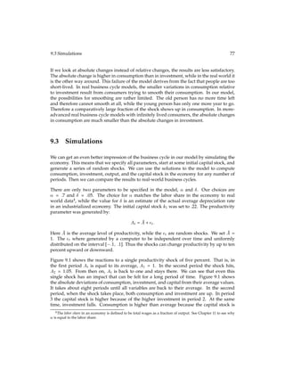
9.3 Simulations
We can get an even better impression of the business cycle in our model by simulating the
economy. This means that we specify all parameters, start at some initial capital stock, and
generate a series of random shocks. We can use the solutions to the model to compute
consumption, investment, output, and the capital stock in the economy for any number of
periods. Then we can compare the results to real-world business cycles.
There are only two parameters to be specified in the model, and Æ. Our choices are
= :7 and Æ = :05. The choice for matches the labor share in the economy to real
world data4
, while the value for Æ is an estimate of the actual average depreciation rate
in an industrialized economy. The initial capital stock k1 was set to .22. The productivity
parameter was generated by:
At = Ā+ t:
Here Ā is the average level of productivity, while the t are random shocks. We set Ā =
1. The t where generated by a computer to be independent over time and uniformly
distributed on the interval [ :1; :1]. Thus the shocks can change productivity by up to ten
percent upward or downward.
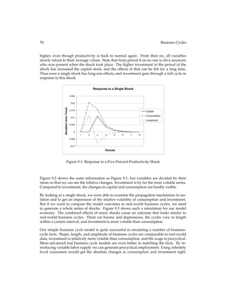
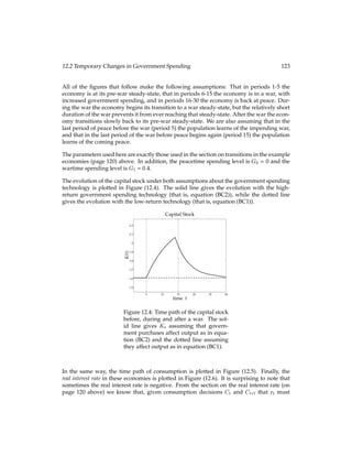
Figure 9.1 shows the reactions to a single productivity shock of five percent. That is, in
the first period At is equal to its average, A1 = 1. In the second period the shock hits,
A2 = 1:05. From then on, At is back to one and stays there. We can see that even this
single shock has an impact that can be felt for a long period of time. Figure 9.1 shows
the absolute deviations of consumption, investment, and capital from their average values.
It takes about eight periods until all variables are back to their average. In the second
period, when the shock takes place, both consumption and investment are up. In period
3 the capital stock is higher because of the higher investment in period 2. At the same
time, investment falls. Consumption is higher than average because the capital stock is
4The labor share in an economy is defined to be total wages as a fraction of output. See Chapter 11 to see why
is equal to the labor share.

191. 78 Business Cycles
higher, even though productivity is back to normal again. From then on, all variables
slowly return to their average values. Note that from period 4 on no one is alive anymore
who was present when the shock took place. The higher investment in the period of the
shock has increased the capital stock, and the effects of that can be felt for a long time.
Thus even a single shock has long-run effects, and investment goes through a full cycle in
response to this shock.
Response to a Single Shock
-0.01
-0.005
0
0.005
0.01
0.015
0.02
0.025
1 2 3 4 5 6 7 8
Periods
Deviation
from
Trend
Capital
Consumption
Investment
Figure 9.1: Response to a Five-Percent Productivity Shock
Figure 9.2 shows the same information as Figure 9.1, but variables are divided by their
mean so that we can see the relative changes. Investment is by far the most volatile series.
Compared to investment, the changes in capital and consumption are hardly visible.
By looking at a single shock, we were able to examine the propagation mechanism in iso-
lation and to get an impression of the relative volatility of consumption and investment.
But if we want to compare the model outcomes to real-world business cycles, we need
to generate a whole series of shocks. Figure 9.3 shows such a simulation for our model
economy. The combined effects of many shocks cause an outcome that looks similar to
real-world business cycles. There are booms and depressions, the cycles vary in length
within a certain interval, and investment is more volatile than consumption.
Our simple business cycle model is quite successful in emulating a number of business-
cycle facts. Shape, length, and amplitude of business cycles are comparable to real-world
data, investment is relatively more volatile than consumption, and the wage is procyclical.
More-advanced real business cycle models are even better in matching the facts. By in-
troducing variable labor supply we can generate procyclical employment. Using infinitely
lived consumers would get the absolute changes in consumption and investment right.

192. 9.3 Simulations 79
Response to a Single Shock
0
0.5
1
1.5
2
2.5
1 2 3 4 5 6 7 8
Periods
Relative
Deviation
Capital
Consumption
Investment
Figure 9.2: Relative Changes in Response to a Five-Percent Pro-
ductivity Shock
State-of-the-art real business cycle models match most business cycle facts, and when fed
with measured productivity shocks, they generate cycles that explain about 70% of the size
of actual business cycles.
This success has led some researchers to the conclusion that business cycles are exactly
what standard economic theory predicts. In the presence of shocks to production possi-
bilities, optimal adjustments of households and firms within an efficient market system
generate just the pattern of fluctuations that is observed in the real world. From this per-
spective, business cycles are no miracle at all. We would be surprised if there were no
business cycles!
Even though technology shocks combined with efficient markets appear to provide a con-
vincing explanation for business cycles, it cannot be ruled out that other shocks or propa-
gation mechanisms also play a role. After all, real business cycle theory does not account
for 100% of the amplitude of actual business cycles, so there have to be other factors as well.
Other types of shocks can be analyzed within the real business cycle framework. There are
also a number of models that emphasize other propagation mechanisms. The Keynesian
model of output determination is the most prominent example5
but models that combine
monetary shocks with frictions in the financial sector have also received a lot of attention
lately. However, so far none of these models matches the ability of the real business cycle
model to mimic actual economic fluctuations.
5See Barro’s Chapter 20 for a discussion of that model. For a critique of the real business cycle model from
a Keynesian perspective, try the following article: Mankiw, N. Gregory. 1989. “Real Business Cycles: A New
Keynesian Perspective”. Journal of Economic Perspectives 3(3): 79-90.

193. 80 Business Cycles
Many Shocks
0
0.5
1
1.5
2
2.5
1 2 3 4 5 6 7 8 9 10 11 12 13
Periods
Relative
Deviation
Capital
Consumption
Investment
Figure 9.3: Capital, Consumption, and Investment with Many
Shocks
Variable Definition
ct
t Consumption of generation t when young
ct
t+1 Consumption of generation t when old
u() Utility function
kt Capital saved in t and used in t+ 1
lt Labor
wt Wage
rt Rental rate of capital
f() Production parameter
At Productivity parameter
Parameter in the production function
Æ Depreciation rate
Ct Aggregate consumption
It Aggregate investment
Yt Aggregate output
Random shock
Table 9.1: Notation for Chapter 9

194. Exercises 81
Exercises
The following exercises make up a project that can be done in groups or individually.
Exercise 9.1 (Moderate)
As the word “cycle” indicates, for a long time economists thought of business cycles as reg-
ular, recurrent events. The length and severity of business cycles was thought to be mostly
constant. For example, the typical length of one full cycle (from boom through recession
back to boom) was supposed to be between four and seven years. In this question you will
examine the actual business cycles of a country of your choice and examine whether they
seem to follow a regular pattern.
The first thing to do is to get the necessary data. Business cycles are roughly defined as
deviations of real GDP from trend. Therefore you will need to acquire data on real GDP for
some country. A good source is the Penn World Tables, a set of standardized measures of
economic activity for most countries in the world. You can access the World Tables through
a website at the University of Toronto. The address is:
http://arcadia.chass.utoronto.ca/pwt/
Once you are there, select “Alphabetical List of Topics”, then “Real GDP per capita in con-
stant dollars using chain index”, then click on the country of your choice (not the United
States), then use the “Submit Query” button to get the data. Load the data into a spread-
sheet, and you are ready to go.
The first step is to compute the trend component of GDP. Good methods for computing
the trend of a time series require a relatively high amount of complicated computations.
Therefore we will offer you an ad hoc, quick-and-dirty method of computing the trend.
Once we get to the business cycles, it turns out that this method works sufficiently well
for our purposes. We will use GDPt to denote real GDP at time t. The computation of the
trend proceeds in steps:
Compute the growth rate of GDP for each year. In terms of your spreadsheet, let us
assume that column A is year and column B is real GDP. The first year is in row one.
Now you can put the growth rates into column C. Put the growth rate from year 1 to
2 into cell C1, and so on.
From now on, we are going to apply a method called exponential smoothing to get
smooth versions of our data. Assume you want to get a smooth version of a times
series xt. Let us call the smooth version x̂t. Basically, the x̂t are computed as a forecast
based on past observations of xt. The first x̂t is set equal to the first xt: x̂1 = x1.
From then on, the forecasts for the next period are computed as an average of the last
forecast and the actual value: x̂t+1 =

195. x̂t + (1

196. )xt, where

197. is a number between

198. 82 Business Cycles
zero and one. If you plug this formula recursively into itself, you will see that each
x̂t is a weighted average of past xt.
Let us now put a smooth growth rate into column D. Since x̂1 = x1, the first smooth
value is equal to the original value: D1=C1. For the next value, we apply the smooth-
ing formula. We recommend that you set

199. to .5: D2=.5*D1+.5*C1. In the same way,
you can get the other smoothed growth rates. For future reference, We will call the
smooth growth rates ĝt.
In the next step, we are going to apply the same method to real GDP, but additionally
we will use the smooth growth rates we just computed. This smooth real GDP is
the trend we are looking for, and we will place it in column E. As before, in the first
year the smooth version is identical to the original one: Trend1 = GDP1, thus E1=B1.
From then on, we get the trend in the next period by averaging between the trend
and the actual value (as before), but also applying the smooth growth rates we just
computed. If we do not do that, our trend will always underestimate GDP. From year
two on the formula is therefore:
Trendt+1 = (1 + ĝt)(0:5)Trendt + (0:5)GDPt:
In terms of the spreadsheet, this translates into E2=(1+D1)*(.5*E1+.5*B1), and so on.
This completes the computation of the trend. Plot a graph of GDP and its trend. If the
trend does not follow GDP closely, something is wrong. (Document your work, providing
spreadsheet formulas, etc.)
Exercise 9.2 (Moderate)
Now we want to see the cyclical component of GDP. This is simply the difference between
GDP and its trend. Because we are interested in relative changes, as opposed to absolute
changes, it is better to use log-differences instead of absolute differences. Compute the
cyclical component as ln(GDP) ln(Trend). Plot the cyclical component. You will see
the business cycles for which we have been looking. (Document your work, providing
spreadsheet formulas, etc.)
Exercise 9.3 (Easy)
Now we will examine the cycles more closely. Define “peak” by a year when the cyclical
component is higher than in the two preceding and following years. Define “cycle” as the
time between two peaks. How many cycles do you observe? What is the average length
of the cycle? How long do the shortest and the longest cycles last? Do the cycles look
similar in terms of severity (amplitude), duration, and general shape? (Document your
work, providing spreadsheet formulas, etc.)
Exercise 9.4 (Moderate)
Having seen a real cycle, the next step is to create one in a model world. It turns out that
doing so is relatively hard in a model with infinitely lived agents. There we have to deal
with uncertainty, which is fun to do, but it is not that easy as far as the math is concerned.

200. Exercises 83
Therefore our model world will have people living for only one period. In fact, there is just
one person each period, but this person has a child that is around in the next period, and
so on. The person, let us call her Jill, cares about consumption ct and the bequest of capital
kt+1 she makes to her child, also named Jill. The utility function is:
ln(ct) + Aln(kt+1);
where A 0 is a parameter. Jill uses the capital she got from her mother to produce
consumption ct and investment it, according to the resource constraint:
ct + it =
p
Bkt + t;
where B 0 is a parameter, and t a random shock to the production function. The shock
takes different values in different periods. Jill knows t once she is born, so for her it is just
a constant. The capital that is left to Jill the daughter is determined by:
kt+1 = (1 Æ)kt + it;
where the parameter Æ, the depreciation rate, is a number between zero and one. This just
means that capital tomorrow is what is left over today after depreciation, plus investment.
Compute Jill’s decision of consumption and investment as a function of the parameters kt,
and t.
Exercise 9.5 (Moderate)
If we want to examine the behavior of this model relative to the real world, the next step
would be to set the parameters in a way that matches certain features of the real world.
Since that is a complicated task, we will give some values to you. B is a scale parameter
and does not affect the qualitative behavior of the model. Therefore we set it to B = :1.
Æ is the depreciation rate, for which a realistic value is Æ = :05. A determines the relative
size of ct and kt in equilibrium. A rough approximation is A = 4. Using these parameters,
compare the reactions of ct and it to changes in t. (Use calculus.)
Exercise 9.6 (Moderate)
In the last step, you will simulate business cycles in the model economy. All you need to
know is the capital k1 at the beginning of time and the random shocks t. As a starting capi-
tal, use k1 = 3:7. You can generate the random shocks with the random number generator in
your spreadsheet. In Excel, just type “=RAND()”, and you will get a uniformly distributed
random variable between zero and one. Generate 50 such random numbers, and use your
formulas for ct and it and the equation for capital in the next period, kt+1 = (1 Æ)kt + it,
to simulate the economy. Plot consumption and investment (on a single graph). How does
the volatility of the two series compare? Plot a graph of GDP, that is, consumption plus in-
vestment. How do the business cycles you see compare with the ones you found in the real
world? You don’t need to compute the length of each cycle, but try to make some concrete
comparisons.

201. 84 Business Cycles
Exercise 9.7 (Easy)
Read the following article: Plosser, Charles. 1989. “Understanding Real Business Cycles”.
Journal of Economic Perspectives 3(3): 51-78. Plosser is one of the pioneers of real business
cycle theory. What you have done in the previous exercises is very similar to what Plosser
does in his article. His economy is a little more realistic, and he gets his shocks from the
real world, instead of having the computer draw random numbers, but the basic idea is
the same.
Describe the real business cycle research program in no more than two paragraphs. What
question is the theory trying to answer? What is the approach to answering the question?
Exercise 9.8 (Moderate)
What does Plosser’s model imply for government policy? Specifically, can the government
influence the economy, and is government intervention called for?

202. Chapter 10
Unemployment
The study of unemployment is usually cast as the study of workers. Several theories seek
to explain why the labor market might not clear at a particular wage. Among these are
“search” models, in which unemployed people are in the process of looking for work. One
such model is presented in Chapter 10 of the Barro textbook. More-sophisticated theo-
ries attempt to explain unemployment as the breakdown in a matching process between
workers and jobs. Public discussions of unemployment often conflate the two.
In this chapter we will discuss some exciting new research on the statistical characteristics
of jobs and employment in the United States. We will not attempt to provide theoretical ex-
planations for the observed statistical patterns; rather, we will concentrate on the statistics
themselves. The primary source for the material in this chapter is Job Creation and Destruc-
tion, by Davis, Haltiwanger, and Schuh.1
Hereafter, we will refer to this book simply as
“DHS”. The book synthesizes research based on some important data sets regarding jobs
and employment. This chapter can provide only a very broad outline of the book, and the
interested reader is strongly encouraged to obtain his or her own copy. The book is short,
accessible, and every page contains something worth knowing.
The authors use two previously untapped sets of data regarding manufacturing employ-
ment in the United States. They present evidence that the main statistical regularities of
their data sets are also present in service industries and across countries. The data sets give
them the number of jobs (defined as filled employment positions) at different establishments
(roughly, factories) over time. Most importantly, they are able to track gross job flows over
time, i.e., how many jobs are created and how many are destroyed at each establishment.
Standard measures track only net job flows, i.e., the difference between the number created
and the number destroyed. It turns out that net flows conceal an enormous amount. For
1The complete citation is: Davis, Steven J., John C. Haltiwanger, and Scott Schuh. Job Creation and Destruction.
Cambridge, Mass.: MIT Press. 1996.

203. 86 Unemployment
example, if we knew that the number of jobs in the U.S. grew 3% from 1998 to 1999, from
say 100 million to 103 million, we would know the net change in jobs, but nothing about
the gross changes in jobs. How many jobs were created? How many destroyed? Until
DHS, there were simply no good answers to those questions.
The authors find that in a typical year 10% of jobs are created and that a roughly equal
number are destroyed. The authors are also able to track job creation and destruction over
the business cycle, and they find that job creation falls slightly during recessions, whereas
job destruction grows strongly. Their data sets contain information about the nature of
the establishments, so they are able to track job creation and destruction by employer and
by factory characteristics. They convincingly explode one of the shibboleths of modern
American political discourse: the myth of small-business job creation. It turns out that
most jobs are created (and destroyed) by large, old plants and firms. This insight alone
makes the book worth reading.
We begin with a primer on the notation used in DHS and then turn to a brief overview of
the main conclusions of the book.
10.1 Job Creation and Destruction: Notation
Basic Notation
Variables in DHS can take up three subscripts. For example, the total number of filled
employment positions at a plant is denoted Xest, where edenotes the establishment (that is,
the plant), s denotes the sector (for example, the garment industry) and t denotes the time
period (usually a specific year). If you find this notation confusing, ignore the differences
among the first two subscripts e and s and just think of them as denoting the same thing:
establishments. Capital letters will denote levels and lower-case letters will denote rates.
The words “plant” and “establishment” mean the same thing. A job is defined as a filled
employment position; no provision is made for considering unfilled positions.
Jobs are created when a plant increases the number of jobs from one period to the next,
while jobs are destroyed when a plant decreases the number of jobs from one period to the
next. Gross job creation is the sum of all new jobs at expanding and newly-born plants, while
gross job destruction is the sum of all the destroyed jobs at shrinking and dying plants. Let
Xest denote the number of jobs at establishment ein sector s at time t, and let S+
t be the set
of establishments that are growing (i.e., hiring more workers) between periods t 1 and t.
Then gross job creation is:
Cst =
X
e2S+
t
Xest;

204. 10.1 Job Creation and Destruction: Notation 87
where is the difference operator:
Xest Xest Xes;t 1:
In words, Cst is the total number of new jobs at expanding and newly born plants in sector
s between periods t 1 and t. Next we turn to job destruction. Let St be the set of
establishments that are shrinking between periods t 1 and t. Then gross job destruction
is:
Dst =
X
e2St
jXestj:
In words, Dst is the total number of all the jobs lost at shrinking and dying plants in sector
s between periods t 1 and t. The absolute-value operator guarantees that Dst will be a
positive number.
Next, we need a measure for the size of a plant. DHS use the average number of jobs
between the current period and the last. For some establishment e in sector s at time t,
DHS define its size Zest as follows:
Zest 1
2
Xest + Xes;t 1
:
Notice that the size in period t contains employment information for both periods t and
t 1.
Suppose we discover that ten-thousand jobs were created in the mining sector in 1996. In
our notation, we would write that as: Cm;1996 = 10,000, where m is for “mining”. This
information would be more useful if compared with some measure of the number of jobs
already present in the mining sector, which is what we call a rate. Then we could say, for
example, that the gross rate of job creation in the mining sector was 10% in 1996.
The rate of employment growth at the plant level is defined as:
gest =
Xest
Zest
:
(10.1)
Let Zst be the sum of all the plant sizes in sector s. Then the rate of job creation in a sector
is defined as:
cst =
Cst
Zst
:
(10.2)
The rate of job destruction is defined similarly:
dst =
Dst
Zst
:
(10.3)
Notice that if some plant i dies between t 1 and t (so that Xi;t 1 0 but Xit = 0), then
the growth rate of the plant will be git = 2, while if plant i is born in t (so that Xi;t 1 = 0
and Xit 0), then the growth rate of the plant will be git = 2.

205. 88 Unemployment
A Simple Example
Consider an economy with only one sector and three plants, P1, P2, and P3. The following
tables list the total employment figures for these three plants as well as: the gross levels
of job creation and destruction at the plant level, average plant size, and gross rates of job
creation and destruction.
Year XP1;t XP2;t XP3;t Total
1991 200 100 0 300
1992 0 300 200 500
Plant i P1 P2 P3 Total
Zi;1992 100 200 100 400
Xi;1992 -200 200 200 200
Ci;1992 0 200 200 400
Di;1992 200 0 0 200
gi;1992 -2.0 1.0 2.0
Notice that plant P1 died between 1991 and 1992, so its growth rate was 2, the same as
it would have been for any plant that died. Plant P3 was born between 1991 and 1992,
so its growth was 2, the same as it would have been for any plant that was born. This is
because of the somewhat non-standard definition of plant size chosen by DHS. (See equa-
tion (10.1).) The economy went from 300 jobs in 1991 to 500 jobs in 1992, so it added 200
net jobs. However, two plants expanded, adding 200 jobs each, while one plant contracted,
destroying 200 jobs. Thus gross job creation was 400 jobs, and gross job destruction was
200 jobs.
In 1992 the sizes Zi;1992 of the three plants were 100, 200, and 100 jobs, respectively, so
the aggregate plant size Z1992 was 400. Recall, S+
1992 is the set of plants that were growing
between 1991 and 1992, so S+
1992 = f2;3g. The rate of job creation c1992 for this economy
was:
c1992 =
C1992
Z1992
=
P
i2S+
1992
Xi;1992
Z1992
=
200 + 200
400
= 1:
Now, recall that S1992 was the set of plants that were shrinking between 1991 and 1992.
Using the same formulation, we can calculate the economy-wide rate of job destruction as:
d1992 =
D1992
Z1992
=
P
i2S1992
jXi;1992j
Z1992
=
j 200j
400
= 0:5:

206. 10.1 Job Creation and Destruction: Notation 89
Job Reallocation, Net Job Creation, and Persistence
Let Rst be the sum of the number of jobs created and the number of jobs destroyed in sector
s between periods t 1 and t. We call Rst the level of job reallocation in sector s at time t.
Formally:
Rst = Cst + Dst:
Note that Rst is an upper bound for the number of workers who have to switch jobs to
accommodate the redistribution of employment positions across plants.
We define the employment status of a citizen to be: “employed”, “unemployed”, or “not in
the workforce”. With that in mind, consider the previous example. For that one-sector
economy, 600 jobs were reallocated. Imagine that all of the 400 newly created positions
were filled with workers just entering the workforce and that none of the workers at the
200 destroyed jobs found employment. Then 600 workers changed employment status. Of
course, if some of the workers at the 200 destroyed jobs had been hired to fill the newly
created jobs, then the number of workers changing employment status would have been
lower.
As before, we convert the level of job reallocation into a rate by dividing by our measure
of plant size Zst. Formally, the rate of job reallocation in sector sat time tis defined as:
rst Rst
Zst
=
Cst + Dst
Zst
= cst + dst:
Let NETst be the difference between the gross levels of job creation and destruction in
sector sat time t:
NETst = Cst Dst:
This is the net level of job creation. Note that when job destruction is greater than job
creation, NETst will be negative. In the simple example above, NET1992 = 200. Let netst be
the net rate of job creation in sector s at time t. Formally:
netst = cst dst:
Now we are interested in creating a measure of the persistence of the changes in employ-
ment levels at establishments. We will first define a simple counting rule for determining
how many of the new jobs created at a plant are still present after j periods, where j is an
integer greater than or equal to one. Consider some plant i in year t 1 with Xi;t 1 = 100
and Xit = 110. Thus Cit = 10, i.e., ten jobs were created (in gross) at plant iin year t.
Now consider the future year t+ j. If employment Xi;t+j at plant i in the year t+ j is 105,
we say that five of the new jobs created at plant iin the year thave survived for j periods.
If Xi;t+j 99, we say that zero of the new jobs have survived. If Xi;t+j 110, we say that
all ten of the new jobs have survived.

207. 90 Unemployment
Let Æit(j) be the number of new jobs created at plant i in year t that have survived to year
t + j, using the counting rule defined above. The level of job persistence Pc
it(j) at plant i
between periods t and t + j is defined as the number of jobs created in year t that exist in
all of the periods between t and t+ j. Formally:
Pc
it(j) = min fÆit(1);Æit(2);::: ;Æit(j)g:
The rate of job persistence can be calculated by summing over all new and expanding
establishments at time tand dividing by gross job creation at t. Using the fact that we have
defined S+
t to be the set of growing plants, we formally define the rate of job persistence as
follows:
pc
t(j) =
X
i2S+
t
Pc
it(j)
Cst
:
Now we work through an example in order to fix ideas. The following chart gives employ-
ment levels for a firm between 1990 and 1995. Xt denotes the number of jobs at the plant
in the year t, where all other subscripts have been dropped for convenience, and Æ1991(j)
gives the number of jobs created in 1991 that still exist in the period t+ j.
Year Employment Persistent jobs from 1991
1990 X1990 = 100 —
1991 X1991 = 110 —
1992 X1992 = 109 Æ1991(1) = 9
1993 X1993 = 108 Æ1991(2) = 8
1994 X1994 = 107 Æ1991(3) = 7
1995 X1995 = 108 Æ1991(4) = 8
We see that for this plant there were seven jobs that were created in 1991 and were also
present in all periods from 1991 to 1995. Accordingly, Pc
1991(4) = 7. The subtle point is that
one of the jobs of the 108 in 1995 was not one of those created in 1991.
Worker Reallocation and Excess Job Reallocation
We define the level of worker reallocation WRt at time t to be the number of workers who
change employment status or place of employment between periods t 1 and t. There
is no way to extract WRt precisely from the data, since the data concentrate on jobs, not
workers. However, we can provide upper and lower bounds on WRt from the data on
jobs.
Our job reallocation measure Rt may overstate the number of workers who change status
or position. Consider a worker whose job is destroyed and then finds employment later
within the sample period at a newly created job. This worker is counted twice in calculating

208. 10.2 Job Creation and Destruction: Facts 91
Rt. Only in the special case that all fired workers fail to find reemployment in the survey
period would WRt = Rt. Hence Rt provides an upper bound on WRt.
The minimum bound on WRt is maxfCt;Dtg. That is, if 75 jobs were created economy-
wide and 50 were destroyed, we know that at least 75 workers had to change employment
status or place of employment. Imagine that all 50 workers whose jobs were destroyed
found employment at the newly created jobs. Then 25 other workers would have had
to be drawn in to fill the remaining 25 new jobs. Hence the 50 fired workers changed
place of employment and the 25 new workers changed employment status, moving from
unemployed to employed.
10.2 Job Creation and Destruction: Facts
In this section we sketch briefly only the high points of the results in DHS. To answer the
exercises at the back of this chapter, you will need to consult the text directly.
Over the sample period 1973-1988, the net manufacturing job creation rate (ct dt) aver-
aged -1.1%. This basic fact obscures the variation of job creation and destruction over the
business cycle, by industry and by plant characteristic. In this section, we hit some of the
high points.
The average annual rate of job destruction dt in manufacturing was 10.3%, and the average
rate of job creation ct was slightly lower at 9.1%, so the average rate of job reallocation was
19.4%. The rate of job creation hit a peak of 13.3% in the recovery year of 1984, while the rate
of job destruction peaked at 14.5% and 15.6% in the recession years of 1982-83. This points
to the striking cyclical nature of job creation and destruction: in recessions job destruction
spikes well above its mean, while job creation does not fall that much. Moreover, most of
the job creation and destruction is concentrated in plants that open or close, rather than in
plants that change size.
When DHS look at gross job flows across industries, they find that rates of job reallocation
are uniformly high, i.e., all industries create and destroy lots of jobs. However, high-wage
industries tend to have smaller gross job flows than low-wage industries. Finally, they find
that the degree to which an industry faces competition from imports does not significantly
affect job destruction. (For your information, imports make up less than 13% of the market
for 80% of U.S. industries.)
Examining gross job flows by employer characteristics reveals that most jobs are not cre-
ated by small business but rather by large, old firms. The pervasive myth of small-business
job creation is fed by bureaucratic self-interest and by some elementary statistical errors.
Understanding these errors is an instructive exercise in its own right and one of the most
interesting parts of the DHS book.

209. 92 Unemployment
Variable Definition
Xest Number of filled employment positions (jobs) at
plant e, sector s, period t
S+
t Set of plants that grew between periods t 1 and
t
S+
t Set of plants that shrunk between periods t 1
and t
Cst Gross job creation
Dst Gross job destruction
Zest Size of employment of plant e, sector s, period t
gest Plant-level rate of employment growth
cst Rate of job creation
dst Rate of job destruction
Rst Level of job reallocation
rst Rate of job reallocation
NETst Net jobs created in sector sat time t
netst Net rate of creation of jobs in sector s at time t
Pc
t (j) The number of jobs created in period t still pres-
ent j periods later
pc
t(j) Rate of the persistence of job creation
WRt Level of worker reallocation
Table 10.1: Notation for Chapter 10
Finally, we touch on one last insight. Well-diversified plants tend to be more likely to sur-
vive recessions than single-output plants. This makes sense, since by producing a portfolio
of products, a plant can spread the risk that a recession will completely stop demand for
all of its output.
Exercises
Exercise 10.1 (Moderate)
Answer: True, False, or Uncertain, and explain.
1. “Did you know that America’s 22 million small businesses are the principal source
of new jobs?” (Source: Web page of the Small Business Administration.)
2. “In the next century, 20% of the population will suffice to keep the world economy

210. Exercises 93
going.... A fifth of all job-seekers will be enough to produce all the commodities
and to furnish the high-value services that world society will be able to afford” the
remaining 80% will be kept pacified by a diet of “Tittytainment”. (Source: Martin,
Hans-Peter and Harald Schumann. The Global Trap. New York: St Martin’s Press.
1996.)
Exercise 10.2 (Easy)
The plant-level rate of employment growth is defined as:
gest =
Xest
Zest
;
where:
Xest = Xest Xes;t 1:
That is, Xest is the change in employment at plant ein sector sfrom t 1 to t. Show that
gest = 2 for all plants that are born between t 1 and t, and show that gest = 2 for all
plants that die between t 1 and t.
Exercise 10.3 (Easy)
Show the following:
cst =
X
e2S+
Zest
Zst
gest; and:
netst =
X
e2S
Zest
Zst
gest:
Here cst is the average rate of job creation of all plants in sector s. What does the term
Zest=Zst mean?
Exercise 10.4 (Moderate)
For the purposes of this exercise, assume that you have data on annual national job creation
Ct and job destruction Dt for N years, so t = 1 :::N. Show that if annual national job
reallocation Rt and net job creation NETt have a negative covariance, then the variance of
job destruction must be greater than the variance of job creation. Recall the definition of
variance of a random variable X for which you have N observations, fxigN
i=1:
var(X) =
1
N
N
X
i=1
(xi x̄)2
;
where x̄ is the mean of X. Similarly, recall the definition of the covariance of two variables
X and Y. If there are N observations each, fxi;yigN
i=1, then:
cov(X;Y) =
1
N
N
X
i=1
(xi x̄)(yi ȳ):
These definitions and the definitions of NETt and Rt provide all the information necessary
to answer this exercise.

211. 94 Unemployment
Exercise 10.5 (Easy)
Consider the employment statistics in chart below. Compute each of the following five
measures: (i) the economy-wide rate of job creation ct; (ii) the economy-wide rate of job
destruction dt; (iii) the net rate of job creation nett; (iv) the upper bound on the number of
workers who had to change employment status as a result of the gross job changes; and
(v) the lower bound on the number of workers who had to change employment status as a
result of the gross job changes for each each of the years 1991, 1992, 1993, 1994, and 1995.
Year X1;t X2;t X3;t ct dt netst UB LB
1990 1000 0 500
1991 800 100 800
1992 1200 200 700
1993 1000 400 600
1994 800 800 500
1995 400 1200 600
1996 200 1400 600
1997 0 2000 500
Exercise 10.6 (Moderate)
For each of the following statements, determine if it is true, false or uncertain and why. If
possible, back your assertions with specific statistical evidence from DHS.
1. Foreign competition is destroying American manufacturing jobs.
2. Robots and other capital improvements are replacing workers in factories.
3. Most job creation occurs at plants that grow about 10% and most job destruction
occurs at plants that shrink about 10%.
4. Diversified plants are better able to withstand cyclical downturns.
5. Every year, high-wage manufacturing jobs are replaced by low-wage manufacturing
jobs.

212. Chapter 11
Economic Growth
This chapter examines the determinants of economic growth. A startling fact about eco-
nomic growth is the large variation in the growth experience of different countries in re-
cent history. Some parts of the world, like the United States or Western Europe, experi-
enced sustained economic growth over a period of more than 100 years, so by historical
standards these countries are now enormously wealthy. This is not only true in absolute
terms (i.e., GDP), but also if we measure wealth as income per capita (i.e., GDP per person).
In contrast, there are countries where even today large parts of the population live close
to the subsistence level, much the same as Europeans and Americans did some hundreds
of years ago. Also, a group of countries that used to be relatively poor around the time of
World War II managed to achieve even higher growth rates than the western industrialized
countries, so their per capita incomes now approach those of western countries. Most of
the members of this group are located in East Asia, like Japan, Singapore, Hong Kong, and
so on.
It proves to be difficult to explain these different growth experiences within a single model.
There are models that provide an explanation for the growth experience of the now indus-
trialized countries, but most of these models fail to explain why much of the world is still
poor. Models that seek to explain the difference between rich and poor countries are less
successful at reproducing the growth facts for industrialized countries. We will therefore
approach the topic of economic growth from a number of different angles. In Section 11.1
we present a number of facts about economic growth, facts that we will seek to explain
with our growth models. Section 11.2 introduces the Solow growth model, a classic in the
theory of economic growth. This model is quite successful at matching a number of facts
about growth in industrialized countries. Section 11.3 introduces growth accounting, an
empirical application of the Solow framework. This kind of accounting can be used to de-
termine the sources of growth for a given country. In Section 11.4 we turn to the question
why some countries are still poor today. A complete answer to this question is beyond the
scope of this book; in fact, it is fair to say that a satisfactory answer has not been found yet.

213. 96 Economic Growth
Therefore we concentrate on only one important aspect of the growth experience of poor
countries: the relationship between fertility, human capital, and growth.
11.1 Growth Facts
If we look at the group of industrialized countries only, we can identify a number of empir-
ical regularities in the growth process. The British economist Nicholas Kaldor summarized
these regularities in a number of stylized facts. Although he did that more than 50 years
ago, the Kaldor facts still provide an accurate picture of growth in industrialized countries.
Kaldor’s first observation was that both output per worker and capital per worker grow
over time. They also grow at similar rates, so the ratio of the aggregate capital stock to
output or GDP does not change much over time. The return to capital, i.e., the interest that
firms have to pay if they rent capital, is almost constant over time. Finally, the labor share
and capital share are almost constant. The labor share is the fraction of output that goes to
workers in the form of wages; it is computed as aggregate labor income divided by GDP.
Similarly, the capital share is given by aggregate payments to capital divided by GDP. No-
tice that the Kaldor facts hold even if we consider long periods of time. For example, the
capital-output ratio and the return to capital are not much different now from what they
were 100 years ago, even though output is much higher now and the goods produced and
the general technology have changed completely.
In addition to the Kaldor facts, another important fact about growth in the industrialized
world is the convergence of per capita GDP of different countries and regions over time.
For example, the relative difference in per capita GDP between the southern and northern
states in the United States has diminished greatly since the Civil War. Similarly, countries
like Germany and Japan that suffered greatly from World War II have grown fast since the
war, so today per capita income in the United States, Japan, and Germany are similar again.
There are no empirical regularities comparable to the Kaldor facts that apply to both indus-
trialized and developing countries. However, we can identify some factors that distinguish
countries that went through industrialization and have a high income today from countries
that remained relatively poor. An explanation of the role of such factors might be an im-
portant step toward understanding the large international differences in wealth. We are
going to focus on the relationship between growth and fertility. Every now industrialized
country has experienced a large drop in fertility rates, a process known as the demographic
transition. All industrialized countries have low rates of population growth. Without im-
migration countries like Germany and Japan would actually shrink. Two centuries ago,
fertility rates were much higher, as they are in most developing countries today. Today,
almost all of the growth in world population takes place in developing countries. We will
come back to these observations in the section on fertility and human capital, but first we
present a model that accounts for the stylized facts about growth in developed countries.

214. 11.2 The Solow Growth Model 97
11.2 The Solow Growth Model
A natural starting point for a theory of growth is the aggregate production function, which
relates the total output of a country to the country’s aggregate inputs of the factors of
production. Consider the neoclassical production function:
Yt = (AtLt)K1
t 1 :
(11.1)
We used a production function of this form already in the chapter on business cycles. Out-
put depends on the aggregate labor input Lt, the aggregate capital input Kt 1, and a pro-
ductivity parameter At. Of course, it is a simplification to consider only three determinants
of output. We could include other factors like land or environmental quality, and our fac-
tors could be further subdivided, for example by distinguishing labor of different quality.
It turns out, however, that a production function of the simple form in equation (11.1) is
all we need to match the stylized facts of economic growth. The production function equa-
tion (11.1) exhibits constant returns to scale, which means that if we double both inputs,
output also doubles. Our choice of a constant-returns-to-scale production function is not
by accident: most results in this section hinge on this assumption.
Equation (11.1) indicates the potential sources of growth in output Yt. Either the inputs
Lt and Kt 1 must grow, or productivity At must grow. If we want to explain economic
growth, we need a theory that explains how the population (i.e., labor), the capital stock,
and productivity change over time. The best approach would be to write down a model
where the decisions of firms and households determine the changes in all these variables.
The consumers would make decisions about savings and the number of children they want
to have, which would explain growth in capital and population. Firms would engage in
research and development, which would yield a theory of productivity growth. However,
doing all those things at the same time results in a rather complicated model.
The model that we are going to present takes a simpler approach. Growth in productivity
and population is assumed to be exogenous and constant. This allows us to concentrate
on the accumulation of capital over time. Moreover, instead of modeling the savings de-
cision explicitly, we assume that consumers invest a fixed fraction of output every period.
Although these are quite radical simplifications, it turns out that the model is rather suc-
cessful in explaining the stylized facts of economic growth in industrialized countries. It
would be possible to write down a model with optimizing consumers that reaches the same
conclusions. In fact, we wrote down that model already: the real business cycle model that
we discussed in Chapter 9 used a neoclassical production function, and the optimal de-
cision of the consumers was to invest a fixed fraction of their output in new capital. To
keep the presentation simple, we will not go through individual optimization problems;
instead, we will assume that it is optimal to save a fixed fraction of output. There are a
number of names for the model. It is either referred to as the Solow model after its inventor
Robert Solow, or as the neoclassical growth model after the neoclassical production function
it uses, or as the exogenous growth model after the fact that there is no direct explanation for
productivity growth.

215. 98 Economic Growth
The law of motion for a variable describes how the variable evolves over time. In the Solow
model, the law of motion for capital is:
Kt = (1 Æ)Kt 1 + It;
(11.2)
where It is investment and Æ is the depreciation rate, which is between zero and one. We
assume that investment is a fixed fraction 0 s 1 of output:
It = sYt = s(AtLt)K1
t 1 :
Productivity and labor grow at fixed rates and
:
At+1 = (1 + )At; and:
Lt+1 = (1 +
)Lt:
We now have to find out how the economy develops, starting from any initial level of
capital K0, and then check whether the model is in line with the stylized facts of economic
growth in industrialized countries.
We assume that there is a competitive firm operating the production technology. We can
check one of the stylized facts, constant labor and capital share, just by solving the firm’s
problem. The profit maximization problem of the firm is:
max
Lt;Kt 1
n
(AtLt)K1
t 1 wtLt rtKt 1
o
:
The first-order conditions with respect to labor and capital yield formulas for wage and
interest:
wt = A
t L 1
t K1
t 1 ; and:
(11.3)
rt = (1 )(AtLt)K
t 1:
(11.4)
We can use these to compute the labor and capital shares in the economy:
wtLt
Yt
=
A
t L 1
t K1
t 1 Lt
(AtLt)K1
t 1
= ; and:
rtKt 1
Yt
=
(1 )(AtLt)K
t 1Kt 1
(AtLt)K1
t 1
= 1 ;
so the labor share is , and the capital share is 1 . Thus both the labor and capital shares
are indeed constant. This result is closely connected to the fact that the production function
exhibits constant returns to scale. Actually, the fact that the labor and capital shares are
about constant is one of the main arguments in favor of using production functions that
exhibit constant returns to scale.
To continue, we have to take a closer look at the dynamics of capital accumulation in the
model. It turns out that this is easiest to do if all variables are expressed in terms of units

216. 11.2 The Solow Growth Model 99
of effective labor AtLt. The product AtLt is referred to as effective labor because increases
in At make labor more productive. For example, At = 2 and Lt = 1 amounts to the same
quantity of effective labor as At = 1 and Lt = 2. When put in terms of units of effective
labor, all variables will be constant in the long run, which will simplify our analysis.
We will use lowercase letters for variables that are in terms of effective labor. That is,
yt = Yt=(AtLt), kt 1 = Kt 1=(AtLt), and it = It=(AtLt). Substituting Yt = ytAtLt and so on
into the production function, equation (11.1), yields:
ytAtLt = (AtLt)(kt 1AtLt)1 ; or:
yt = k1
t 1 :
(11.5)
From the law of motion for capital, equation (11.2), we get the law of motion in terms of
effective labor:
kt(1 + )At(1 +
)Lt = (1 Æ)kt 1AtLt + itAtLt; or:
kt(1 + )(1 +
) = (1 Æ)kt 1 + it:
(11.6)
Finally, investment is determined by:
it = syt = sk1
t 1 :
(11.7)
Plugging equation (11.7) into the law of motion in equation (11.6) yields:
kt(1 + )(1 +
) = (1 Æ)kt 1 + sk1
t 1 ; or:
kt =
(1 Æ)kt 1 + sk1
t 1
(1 + )(1 +
)
:
(11.8)
This last equation determines the development of the capital stock over time. Dividing by
kt 1 yields an expression for the growth rate of capital per unit of effective labor:
kt
kt 1
=
1 Æ + sk
t 1
(1 + )(1 +
)
:
(11.9)
The expression kt=kt 1 is called the gross growth rate of capital per unit of effective labor.
The gross growth rate equals one plus the net growth rate. The growth rates in Chapter 1
were net growth rates.
Since the exponent on kt 1 in equation (11.9) is negative, the growth rate is inversely related
to the capital stock. When a country has a lower level of capital per unit of effective labor,
its capital and hence its output grow faster. Thus the model explains the convergence of
GDP of countries and regions over time.
Since the growth rate of capital decreases in kt 1, there is some level of kt 1 where capital
per unit of effective labor stops growing. We say that the economy reaches a steady state.
Once the economy arrives at this steady state, it stays there forever. Figure 11.1 is a graphi-
cal representation of the growth process in this economy. For simplicity, we assume for the

217. 100 Economic Growth
moment that labor and productivity are constant, =
= 0. In that case, equation (11.8)
simplifies to:
kt = (1 Æ)kt 1 + sk1
t 1 ; or:
kt kt 1 = sk1
t 1 Ækt 1:
The change in capital per unit of effective labor is equal to the difference between invest-
ment and depreciation. Figure 11.1 shows the production function per unit of effective
labor yt = k1
t 1 , investment it = sk1
t 1 , and depreciation Ækt 1. Because the return to capi-
tal is diminishing, investment is a concave function of capital. For low values of capital, the
difference between investment and depreciation is large, so the capital stock grows quickly.
For larger values of capital, growth is smaller, and at the intersection of depreciation and
investment the capital stock does not grow at all. The level of capital per unit of effective
labor at which investment equals depreciation is the steady-state level of capital. In the
long run, the economy approaches the steady-state level of capital per unit of effective la-
bor, regardless of what the initial capital stock was. This is even true if the initial capital
stock exceeds the steady-state level: capital per unit of effective labor will shrink, until the
steady state is reached.
0
0.05
0.1
0.15
0.2
0.25
k 0.37 0.77
delta*k
f(k)
s*f(k)
Figure 11.1: Output, Saving, and Depreciation in the Solow
Model
At the steady state we have kt = kt 1. Using equation (11.8), we see that the steady-state
level of capital per unit of effective labor k̄ has to satisfy:
k̄(1 + )(1 +
) = (1 Æ)k̄ + sk̄1 ;

218. 11.2 The Solow Growth Model 101
which yields:
k̄ =
s
Æ + +
+
1=
:
(11.10)
We can use this equation to compute output, investment, and growth in the steady state.
From equation (11.5), the steady-state level of output per effective labor unit is:
ȳ = k̄1 =
s
Æ + +
+
1
:
The level of output depends positively on the saving rate. From equation (11.7), the steady-
state investment per unit of effective labor is:
ī = s
s
Æ + +
+
1
:
The steady-state growth rate of capital is +
+
:
Kt
Kt 1
=
k̄(1 + )At(1 +
)Lt
k̄AtLt
= 1 + +
+
;
and the growth rate of output equals +
+
as well. This implies that the long-run
growth rate of an economy is independent of the saving rate. With a higher saving rate,
the economy approaches a higher steady state, but the long-run growth rate is determined
by growth in labor and productivity only.
There are still a number of stylized facts left to be checked. First, we will verify that the
return to capital is constant. From equation (11.4), the return to capital is:
rt = (1 )(AtLt)K
t 1 = (1 )
Kt 1
AtLt
:
In the steady state, capital per unit of effective labor is a constant k̄. Therefore the return to
capital in steady state is:
r̄t = (1 )k̄ ;
which is constant since k̄ is constant. On the other hand, the wage is growing in the steady
state, since the productivity of labor increases. The steady-state wage can be computed as:
wt = A
t L 1
t K1
t 1 = At
Kt 1
AtLt
1
= Atk̄1 ; so:
wt+1
wt
=
At+1
At
= 1 + ;
which implies that the wage grows at the rate of technological progress.

219. 102 Economic Growth
The capital-output ratio in steady state is:
Kt 1
Yt
=
k̄AtLt
ȳAtLt
=
k̄
ȳ;
which is a constant. This verifies the last stylized fact of economic growth on our list.
The Solow model succeeds in explaining all stylized facts of economic growth in indus-
trialized countries. The key element of the model is the neoclassical constant-returns pro-
duction function. Since returns to capital alone are decreasing, economies grow faster at
lower levels of capital, until they approach the steady state, where units of effective labor
and capital grow at the same rate. The model also explains why different saving rates in
different industrialized countries do not translate into long-term differences in the growth
rate. The saving rate affects the level of the steady state, but it does not affect the steady-
state growth rate. The capital stock cannot grow faster than effective labor for a long time
because of decreasing returns to capital.
Since the Solow model does well at matching the facts of economic growth, it forms the
basis of many more-advanced models in macroeconomics. For example, our real business
cycle model of Chapter 9 is a Solow model enriched by optimizing consumers and pro-
ductivity shocks. On the other hand, the model works well only for countries that satisfy
the assumptions of constant rates of population growth and technological progress. These
assumptions are justified for industrialized countries, but they are not helpful for under-
standing the early stages of development of a country, which are usually accompanied by
the demographic transition, so exogenous and constant population growth is not a useful
assumption. We will look for possible explanations of fertility decisions below, but be-
fore that, we will introduce growth accounting, a method that allows us to decompose the
growth rate of a country into growth in population, capital, and productivity.
11.3 Growth Accounting
In this section we will use the general framework of the Solow model to compute a de-
composition of the rate of economic growth for a given country. Consider the neoclassical
production function:
Yt = (AtLt)K1
t 1 :
(11.11)
We will interpret Yt as GDP, Lt as the number of workers, Kt 1 as the aggregate capital
stock, and At as a measure of overall productivity. We will be concerned with measuring
the relative contributions of At, Lt, and Kt 1 to growth in GDP. We assume that data for
GDP, the labor force, and the aggregate capital stock are available. The first step is to
compute the productivity parameter At. Solving the production function for At yields:
At =
Y
1
t
LtK
1
t 1
:

220. 11.4 Fertility and Human Capital 103
If were known, we could compute the At right away. Luckily, we found out earlier that
is equal to the labor share. Therefore we can use the average labor share as an estimate
of and compute the At.
Now that At is available, the growth rates in At, Lt and Kt 1 can be computed.1
We can see
how the growth rates in inputs and productivity affect the growth rate of GDP by taking
the natural log of the production function:
ln Yt = ln At + ln Lt + (1 ) ln Kt 1:
(11.12)
We are interested in growth between the years tand t+ k, where k is some positive integer.
Subtracting equation (11.12) at time t from the same equation at time t+ k yields:
ln Yt+k ln Yt = (ln At+k ln At) + (ln Lt+k ln Lt) + (1 )(ln Kt+k 1 ln Kt 1):
Thus the growth rate in output (the left-hand side) is times the sum of growth in produc-
tivity and labor, plus 1 times growth in capital. Using this, we can compute the relative
contribution of the different factors. The fraction of output growth attributable to growth
of the labor force is:
[ln Lt+k ln Lt]
ln Yt+k ln Yt
:
The fraction due to growth in capital equals:
(1 )[ln Kt+k 1 ln Kt 1]
ln Yt+k ln Yt
:
Finally, the remaining fraction is due to growth in productivity and can be computed as:
[ln At+k ln At]
ln Yt+k ln Yt
:
It is hard to determine the exact cause of productivity growth. The way we compute it, it is
merely a residual, the fraction of economic growth that cannot be explained by growth in
labor and capital. Nevertheless, measuring productivity growth this way gives us a rough
idea about the magnitude of technological progress in a country.
11.4 Fertility and Human Capital
In this section we will examine how people decide on the number of children they have.
Growth and industrialization are closely connected to falling fertility rates. This was true
for 19th century England, where industrialization once started, and it applies in the same
way to the Asian countries that only recently began to grow at high rates and catch up with
1See Chapter 1 for a discussion of growth rates and how to compute them.

221. 104 Economic Growth
Western countries. Understanding these changes in fertility should help explain why some
economies start to grow, while others remain poor.
The first economist to think in a systematic way about growth and fertility was Thomas
Malthus. Back in 1798, he published his “Essay on Population”, in which his basic thesis
was that fertility was checked only by the food supply. As long as there was enough to eat,
people would continue to produce children. Since this would lead to population growth
rates in excess of the growth in the food supply, people would be pushed down to the
subsistence level. According to Malthus’s theory, sustained growth in per capita incomes
was not possible; population growth would always catch up with increases in production
and push per capita incomes down. Of course, today we know that Malthus was wrong,
at least as far as the now industrialized countries are concerned. Still, his theory was an
accurate description of population dynamics before the industrial revolution, and in many
countries it seems to apply even today. Malthus lived in England just before the demo-
graphic transition took place. The very first stages of industrialization were accompanied
by rapid population growth, and only with some lag did the fertility rates start to decline.
We will take Malthus’s theory as a point of departure in our quest for explanations for the
demographic transition.
Stated in modern terms, Malthus thought that children were a normal good. When income
went up, more children would be “consumed” by parents. We assume that parents have
children for their enjoyment only, that is, we abstract from issues like child labor. As a
simple example, consider a utility function over consumption ct and number of children
nt of the form:
u(ct;nt) = ln(ct) + ln(nt):
We assume that the consumer supplies one unit of labor for real wage wt and that the cost
in terms of goods of raising a child is p. Therefore the budget constraint is:
ct + pnt = wt:
By substituting for consumption, we can write the utility maximization problem as:
max
nt
fln(wt pnt) + ln(nt)g:
The first-order condition with respect to nt is:
p
wt pnt
+
1
nt
= 0; or:
(FOC nt)
nt =
wt
2p:
(11.13)
Thus the higher the real wage, the more children are going to be produced.
If we assume that people live for one period, the number of children per adult nt deter-
mines the growth rate of population Lt:
Lt+1
Lt
= nt:

222. 11.4 Fertility and Human Capital 105
To close the model, we have to specify how the wage is determined. Malthus’s assumption
was that the food supply could not be increased in proportion with population growth.
In modern terms, he meant that there were decreasing returns to labor. As an example,
assume that the aggregate production function is:
Yt = AtL
t ;
with 0 1. Also assume that the real wage is equal to the marginal product of labor:
wt = AtL 1
t :
(11.14)
We can combine equation (11.14) with the decision rule for the number of children in equa-
tion (11.13) to derive the law of motion for population:
Lt+1
Lt
=
AtL 1
t
2p ; or:
Lt+1 =
AtL
t
2p :
(11.15)
Notice that this last equation looks similar to the law of motion for capital in the Solow
model. The growth rate of population decreases as population increases. At some point,
the population stops growing and reaches a steady state L̄. Using equation (11.15), the
steady-state level of population can be computed as:
L̄ =
AtL̄
2p ; or:
L̄ =
At
2p
1
1
:
In the steady state, we have Lt+1=Lt = nt = 1. We can use this in equation (11.13) to compute
the wage w̄ in the steady state:
1 =
w̄
2p; or:
w̄ = 2p:
Thus the wage in the steady state is independent of productivity At. An increase in At
causes a rise in the population, but only until the wage is driven back down to its steady-
state level. Even sustained growth in productivity will not raise per capita incomes. The
population size will catch up with technological progress and put downward pressure on
per capita incomes.
This Malthusian model successfully explains the relationship between population and out-
put for almost all of history, and it still applies to large parts of the world today. Most
developing countries have experienced large increases in overall output over the last 100
years. Unlike in Europe, however, this has resulted in large population increases rather

223. 106 Economic Growth
than in increases in per capita incomes. Outside the European world, per capita incomes
stayed virtually constant from 1700 to about 1950, just as the Malthusian model predicts.
Something must have changed in Europe in the nineteenth century that made it attractive
to people to have less children, causing fertility rates to fall , so per capita incomes could
start to grow. While these changes are by no means fully understood, we can identify a
number of important factors. We will concentrate on two of them: the time-cost of raising
children, and a quality-quantity tradeoff in decisions on children.
Human capital is a key element of the model that we are going to propose. So far, we con-
sidered all labor to be of equal quality. That might be a reasonable assumption for earlier
times in history, but it certainly does not apply in our time, where special qualifications
and skills are important. In the model, human capital consists of two components. First,
there is innate human capital that is possessed by every worker, regardless of education.
We will denote this component of human capital by H0. This basic human capital reflects
the fact that even a person with no special skill of any kind is able to carry out simple tasks
that require manual labor only. In addition to this basic endowment, people can acquire
extra human capital Ht through education by their parents. Ht reflects special skills that
have to be taught to a worker. The total endowment with human capital of a worker is
H0 + Ht.
To come back to fertility decisions, we now assume that parents care both about the number
nt of their children and their “quality”, or human capital H0 + Ht+1. Preferences take the
form:
u(ct;nt;Ht+1) = ln(ct) + ln(nt(H0 + Ht+1)):
The other new feature of this model is that parents must invest time, rather than goods, to
raise children. In the Malthusian model, p units of the consumption good were needed to
raise a child. We now assume that this cost in terms of goods is relatively small, so it can
be omitted for simplicity. Instead, children require attention. For each child, a fraction hof
the total time available has to be used to raise the child. In addition, the parents can decide
to educate their children and spend fraction et of their time doing that. This implies that
only a fraction 1 hnt et is left for work. If wt is the wage per unit of human capital when
working all the time, the budget constraint is:
ct = wt(H0 + Ht)(1 hnt et):
(11.16)
The right-hand side says that income is the wage multiplied by human capital and the
fraction of time worked. All this income is spent on consumption. We still have to specify
the determination of the human capital of the children. We assume that the extra human
capital of each child Ht+1 depends on: the acquired human capital Ht of that child’s parents,
and the time et the parents spend teaching their children:
Ht+1 =
etHt:
(11.17)
Here
is a positive parameter. The interpretation of equation (11.17) is that parents who
are skilled themselves are better at teaching their children. A person who does not have
any skills is also unable to teach anything to his or her children.

224. 11.4 Fertility and Human Capital 107
We now want to determine how fertility is related to human capital in this model. If we
plug the constraints in equations (11.16) and (11.17) into the utility function, the utility
maximization problem becomes:
max
nt;et
fln(wt(H0 + Ht)(1 hnt et)) + ln(nt(H0 +
etHt))g:
The first-order conditions with respect to nt and et are:
h
1 hnt et
+
1
nt
= 0; and:
(FOC nt)
1
1 hnt et
+
Ht
H0 +
etHt
= 0:
(FOC et)
(FOC nt) can be rewritten as:
hnt = 1 hnt et; or:
et = 1 2hnt:
(11.18)
Using equation (11.18) in (FOC et) allows us to compute the optimal fertility decision:
Ht(1 hnt (1 2hnt)) = H0 + (1 2hnt)
Ht; or:
Hthnt = H0 +
Ht 2
Hthnt; or:
3
Hthnt = H0 +
Ht; or:
nt =
1
3h
H0
Ht
+ 1
:
(11.19)
According to equation (11.19), the key determinant of fertility is human capital Ht. If it
is close to zero, the number of children is very high. If we added a cost of children in
terms of goods to this model, for low values of Ht the outcomes would be identical to the
Malthusian model. However, things change dramatically when Ht is high. Fertility falls,
and if Ht continues to rise, the number of children reaches the steady state: n̄ = 1=(3h).
There are two reasons for this outcome. On the one hand, if human capital increases, the
value of time also increases. It becomes more and more costly to spend a lot of time raising
children, so parents decide to have less of them. The other reason is that people with high
human capital are better at teaching children. That makes it more attractive for them to
invest in the quality instead of the quantity of children.
The model sheds some light on the reasons why today fertility in industrialized countries is
so much lower than that in developing countries. The theory also has applications within a
given country. For example, in the United States teenagers are much more likely to become
pregnant if they are school dropouts. The model suggests that this is not by accident.
People with low education have a relatively low value of time, so spending time with
children is less expensive for them.
The question that the model does not answer is how the transition from the one state to
the other takes place. How did England manage to leave the Malthusian steady state?

225. 108 Economic Growth
In the model, only a sudden jump in Ht over some critical level could perform this task,
which is not a very convincing explanation for the demographic transition. Still, the model
is a significant improvement over theories that assume that population growth rates are
exogenous and constant. More research on this and related questions will be needed before
we can hope to find a complete explanation for the demographic transition and the wide
disparity in wealth around the world.
Variable Definition
Yt Aggregate output
yt Output per unit of effective labor
Lt Aggregate labor input or population
Kt Aggregate capital stock
kt Capital per unit of effective labor
At Productivity parameter
It Aggregate investment
it Investment per unit of effective labor
wt Wage
rt Return on capital
Æ Depreciation rate
Parameter in the production function
u() Utility function
ct Consumption
nt Number of children
p Cost of raising a child, in terms of goods
h Cost of raising a child, in terms of time
et Time spent on educating children
H0 Innate human capital
Ht Acquired human capital
Parameter in the production function for human
capital
Table 11.1: Notation for Chapter 11
Exercises
Exercise 11.1 (Easy)
Suppose the aggregate production technology is Y = 3L:7
K:3
and that L = 150. Both the
labor force and productivity are constant. Assume that the depreciation rate is 10% and that

226. Exercises 109
20% of output is saved and invested each year. What is the steady-state level of output?
Exercise 11.2 (Moderate)
Assume that the Solow model accurately describes the growth experience of Kuwait. As
a result of the Gulf war, much of the capital in Kuwait (oil extracting equipment, vehi-
cles, structures etc.) was destroyed. Answer the following questions, and provide brief
explanations.
What will be the effect of this event on per capita income in Kuwait in the next five
years?
What will be the effect of this event on per capita income in Kuwait in the long run?
What will be the effect of this event on the annual growth rate of per capita income
in Kuwait in the next five years?
What will be the effect of this event on the growth rate of per capita income in Kuwait
in the long run?
Will recovery in Kuwait occur faster if investment by foreigners is permitted, or if it
is prohibited?
Would Kuwaiti workers gain or lose by a prohibition of foreign investment? Would
Kuwaiti capitalists gain or lose?
Exercise 11.3 (Moderate)
In this and the following two exercises, you will apply growth accounting to measure the
determinants of growth in output per worker in a country of your choice. To start, you
need to pick a country and retrieve data on real GDP per worker and capital per worker.
You can get the time series you need from the Penn World Tables. See Exercise 9.1 for
information about how to access this data set. You should use data for all years that are
available.
In Section 11.3, we introduced growth accounting for output growth, while in this exercise
we want to explain growth in output per worker. We therefore have to redo the analysis
of Section 11.3 in terms of output per worker. The first step is to divide the production
function in equation (11.11) by the number of workers Lt, which yields:
Yt
Lt
=
(AtLt)K1
t 1
Lt
=
A
t L
t K1
t 1
L
t L1
t
= A
t
Kt 1
Lt
1
:
(11.20)
Equation (11.20) relates output per worker Yt=Lt to capital per worker Kt 1=Lt. If we use
lower case letters to denote per-worker values (yt = Yt=Lt, kt 1 = Kt 1=Lt), we can write
equation (11.20) as:
yt = A
t k1
t 1 :
(11.21)

227. 110 Economic Growth
Use equation (11.21) to derive a formula for At and to derive a decomposition of growth in
output per worker into growth in capital per worker and productivity growth. You can do
that by following the same steps we took in Section 11.3.
Exercise 11.4 (Moderate)
Compute the productivity parameter At for each year in your sample. For your computa-
tions, assume that 1 = :4. This is approximately equal to the capital share in the United
States, and we assume that all countries use the same production function. In fact, in most
countries measures for 1 are close to .4.
Exercise 11.5 (Moderate)
By using log-differences, compute the growth rate of GDP, productivity, and capital per
worker for each year in your sample. Also compute the average growth rate for these three
variables.
Exercise 11.6 (Moderate)
What percentage of average growth per worker is explained by growth in capital, and
what percentage by productivity growth? For the period from 1965 to 1992, the average
growth rate of output per worker was 2.7% in the United States, and productivity growth
averaged 2.3%. How do these numbers compare to your country? Does the neoclassi-
cal growth model offer an explanation of the performance of your country relative to the
United States? If not, how do you explain the differences?

228. Chapter 12
The Effect of Government
Purchases
In this chapter we consider how governmental purchases of goods and services affect the
economy. Governments tend to spend money on two things: wars and social services.
Barro’s Figure 12.2 shows that expenditures by the U.S. government have comprised a
generally increasing fraction of GNP since 1928, but even today that fraction is nowhere
near the peak it attained during WWII. This pattern is generally repeated across countries.
The taste for social services seems to increase with national wealth, so the governments of
richer countries tend to spend more, as a fraction of GDP, than the governments of poorer
countries, especially during peacetime. Of course, there are exceptions to this pattern.
We will examine government spending in three ways:
1. We shall consider the effect of permanent changes in government spending in order
to think about the secular peacetime increases in spending;
2. We shall consider temporary changes in government spending in order to think about
the effect of sudden spikes like wars;
3. We shall begin an analysis of the effect of government social programs. Since govern-
ment social programs (unemployment insurance, social security systems) are inextri-
cably linked to tax systems, we will defer part of our analysis to the next chapter.
Since we have yet to fully discuss tax policy, for this chapter we will assume that the gov-
ernment levies a very special kind of tax: a lump-sum tax. That is, the government an-
nounces a spending plan and then simply removes that amount of money from the budget
of the representative household. As we shall see in the next chapter, this kind of tax system
does not distort the household’s choices.

229. 112 The Effect of Government Purchases
In the Barro textbook, the government budget constraint, in addition to lump sum taxes,
also contains fiat currency. In this chapter we will assume that the government does not
use the printing press to finance its purchases. In later chapters (especially Chapter 18) we
will examine this effect in much greater detail.
12.1 Permanent Changes in Government Spending
Assume that the government announces a permanent level of government spending, G, to
be levied each period. What is the role of these government expenditures? The govern-
ment provides productive services, such as a court system for enforcing contracts and an
interstate highway system for quickly and cheaply transporting goods. The government
also provides consumption services such as public parks and entertainment spectacles such
as trips to the moon and congressional hearings. We focus on the first role.
How should we model the productive services provided by the government? We shall
analyze a model under two assumptions:
1. Government spending at some constant rate ,
2. The effect of government spending G is augmented by the level of capital, Kt, so
output Y increases by the amount GKt.
In the first case, $100 of government spending increases output by 100 regardless of the
current level of capital, while in the second case, the same $100 boosts output much more
in nations with more capital.
The representative household lives forever and has preferences over consumption streams
fCtg1
t=0 given by:
V(fCtg1
t=0) =
1
X
t=0

230. tU(Ct):
Where U0 0 and U00 0. Here 0

231. 1 reflects impatience. In addition, to keep the
algebra nice, we will say that:

232. =
1
1 + :
Here

233. is the discount factor and the discount rate.
The household has access to a productive technology mapping capital Kt into private out-
put YP
t of:
YP
t = K
t :

234. 12.1 Permanent Changes in Government Spending 113
Total output (and hence income) of the household will be the sum of private output and
government-augmented output, YG
t . Government augmented output will take on one of
two values:
YG
t = G; or:
(12.1)
YG
t = GKt:
(12.2)
Equation (12.1) corresponds to the case of government spending affecting total output the
same amount no matter what the level of capital. Equation (12.2) corresponds to the case
of government spending affecting total output more when the level of capital is high. We
shall examine the effect of G on capital accumulation, aggregate output and consumption
under both of these assumptions.
The household must split total income Yt = YP
t + YG
t into consumption Ct, investment It
and payments to the government of G. Recall that we assumed the government would sim-
ply levy lump-sum taxes. Now we are using that assumption. The household’s resource
constraint is thus:
Ct + It + G Yt:
(12.3)
Finally, there is a law of motion for the capital stock Kt. Each period, a proportion Æ of the
capital stock vanishes due to physical depreciation, so only the remaining (1 Æ) proportion
survives into the next period. In addition, capital may be augmented by investment. Thus
capital evolves according to:
Kt+1 = (1 Æ)Kt + It:
(12.4)
We assume that the representative household begins life with some initial stock of capital
K0 0.
We are interested in writing Ct as a function of next period’s capital stock Kt+1. Combining
equations (12.3) and (12.4) gives:
Ct = K
t + (1 Æ)Kt Kt+1 G+ G; or:
(BC1)
Ct = K
t + (1 Æ)Kt Kt+1 G+ GKt:
(BC2)
The differences between the two equations arises from which version of the government
technology we use, equation (12.1) or (12.2).
Analysis with Equation (BC1)
Let us begin our analysis with the first version of the government spending technology,
equation (12.1). Thus we are using as the relevant budget constraint equation (BC1). The

235. 114 The Effect of Government Purchases
household’s problem becomes:
max
fKt+1g1
t=0
1
X
t=0

236. tU [K
t + (1 Æ)Kt Kt+1 (1 )G] :
We take first-order conditions with respect to the choice of next period’s capital Kj+1 in
some typical period j. Remember that Kj+1 appears in two periods, j and j + 1:

237. jU0(Cj)[ 1] +

238. j+1
U0(Cj+1)
h
K 1
j+1 + 1 Æ
i
= 0:
For all j = 0;1;::: ;1. Here Cj is given by equation (BC1) above. Simplifying produces:
U0(Cj) =

239. U0(Cj+1)[K 1
j+1 + 1 Æ]:
(12.5)
For simplicity (and as in other chapters) we choose not to solve this for the transition path
from the initial level of capital K0 to the steady state level KSS, and instead focus on char-
acterizing the steady state. At a steady state, by definition the capital stock is constant:
Kt = Kt+1 = KSS:
As a result:
Ct = Ct+1 = CSS; and:
It = It+1 = ISS = ÆKSS:
Equation (12.5) at the steady-state becomes:
U0(CSS) =

240. U0(CSS)[KSS
1
+ 1 Æ]:
Simplifying, and using the definition of

241. as 1=(1 + ) produces:
1 + = KSS
1
+ 1 Æ:
We now solve for the steady-state capital level:
KSS =
+ Æ
1
1
:
Notice immediately that, under this formulation of government spending the steady state
capital level is independent of government spending. As we shall see in the next chapter,
this is a direct consequence of the lump-sum tax technology. If the government had to use
a distortionary tax, KSS would be affected by G.
Given KSS, it is easy to calculate the other variables that the household controls: steady-
state private income, YSS
P , consumption CSS, and investment, ISS. From the technology, we
know that YP = K, so:
YSS
P = KSS
:

242. 12.1 Permanent Changes in Government Spending 115
Total output (GDP) is private output YP plus government output YG, or:
YSS = KSS
+ G:
Consumption is, in this case, determined by the budget constraint equation (BC1). At the
steady-state, then:
CSS = KSS
+ (1 Æ)KSS KSS (1 )G:
We can simplify this to produce:
CSS = KSS
ÆKSS (1 )G:
At the steady-state, the household must be investing just enough in new capital to offset
depreciation. Substituting into the law of motion for capital provides:
ISS = ÆKSS:
Now we are ready to determine the effect of government spending on total output, con-
sumption and the capital level. When we think about changing G we are comparing two
different steady states. Thus there may be short-term fluctuations immediately after the
government announces its new spending plan, but we are concerned here with the long-
run effects.
Notice immediately that:
dKSS
dG = 0;
(12.6)
dYSS
dG =
d
dG(YP + YG) = ; and:
(12.7)
dCSS
dG = (1 )G::
(12.8)
That is, total output is increasing in G but consumption is decreasing in G if 1. Thus
1 is an example of crowding out. Think of it this way: the government spends $1000 on
a new factory, which produces 1000 units of new output. The household pays the $1000
in taxes required to construct the new factory, does not alter its capital level and enjoys the
extra output of 1000as consumption. If 1 the household has lost consumption. Thus
output has increased and consumption has decreased.
Why do we automatically assume that 1? This is equivalent to saying that the gov-
ernment is worse at building factories than the private sector. The government may be
the only institution that can provide contract enforcement, police and national defense, but
long history has shown that it cannot in general produce final goods as effectively as the
private sector.
One final note before we turn our attention to the effect of production augmenting gov-
ernment spending. Government transfer payments, in which the government takes money

243. 116 The Effect of Government Purchases
from one agent and gives it to another, fit nicely into this category of expenditure. Trans-
fer payments have absolutely no productive effects, and the government institutions re-
quired to administer the transfer payments systems will prevent the perfect transmission
of money from one agent to another. Since we are working with a representative consumer,
transfer payments appear as taxes which are partially refunded.
Analysis with Equation (BC2)
Now let us consider the effect of government spending whose benefits are proportional to
capital stock. We will use precisely the same analysis as before. except that now consump-
tion Ct as a function of capital Kt and Kt+1 and government spending G will be given by
equation (BC2) above.
The household’s problem becomes:
max
fKt+1g1
t=0
1
X
t=0

244. tU [K
t + (1 Æ + G)Kt Kt+1 G] :
We take first-order conditions with respect to the choice of next period’s capital stock Kj+1
in some typical period j. Remember the trick with these problems: Kj+1 appears twice in
the maximization problem, first negatively in period j and then positively in period j + 1:

245. jU0(Cj)[ 1] +

246. j+1
U0(Cj+1)
h
K 1
j+1 + 1 Æ + G
i
= 0:
For all j = 0;1;::: ;1. Cj is given by equation (BC2). Simplifying produces:
U0(Cj) =

247. U0(Cj+1)[K 1
j+1 + 1 Æ + G]:
(12.9)
Compare this with the previous simplified first-order condition, equation (12.5) above. No-
tice that in equation (12.5) the government spending term Gdoes not appear. Here it does.
This should alert us immediately that something new is about to happen. As before, we
assume a steady state and characterize it. At the steady state:
U0(CSS) =

248. U0(CSS)[KSS
1
+ 1 Æ + G]:
Using our definition of

249. as 1=(1 + ) this becomes:
1 + = KSS
1
+ 1 Æ + G:
Hence the steady-state capital level is:
KSS =
+ Æ G
1
1
:

250. 12.1 Permanent Changes in Government Spending 117
Notice immediately that, under this formulation of government spending the steady-state
capital level is increasing in government spending. If the government were forced to fi-
nance its spending with a distortionary tax this result might not go through.
Given the steady-state capital level, it is easy to calculate the steady-state levels of total
output YSS, consumption CSS and investment, ISS. Since the steady-state capital level, KSS, is
now affected by G, both public output YG and private output YP are in turn affected by
G. Given the production function, we see that:
YSS = KSS
+ KSSG:
From the budget constraint equation (BC2) above, we see that the steady state, consump-
tion is:
CSS = KSS
ÆKSS (1 KSS)G:
As before, the household must be investing just enough to overcome depreciation, to keep
the capital level constant:
ISS = ÆKSS:
Now we can reconsider the effect of government spending on total output, consumption
and the capital level. Some of these derivatives are going to be fairly involved, but if we
break them down into their constituent pieces they become quite manageable.
Begin by defining:
X
+ Æ G:
Note that:
dX
dG =
+ Æ GX:
The steady-state capital stock is:
KSS = X 1
1 ;
so the derivative of the steady-state capital stock with respect to G is:
dKSS
dG =
1
1 X 1
1 1 dX
dG:
Plugging in dX=dG yields:
dKSS
dG =
1
1 X 1
1 1
+ Æ GX
=
1
1
+ Æ GX 1
1
=
1
1
+ Æ GKSS:
(12.10)

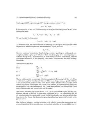
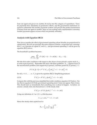
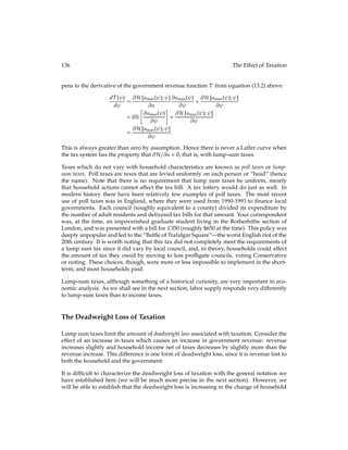
251. 118 The Effect of Government Purchases
Armed with this result we can tackle the other items of interest. First, consider the effect of
increased spending on aggregate output:
dYSS
dG =
d
dG(YSS
P + YSS
G)
=
d
dG (KSS
+ GKSS)
= KSS
1 dKSS
dG + GdKSS
dG
= KSS
1 1
1
+ Æ GKSS + G 1
1
+ Æ GKSS
=
1
1
+ Æ G [KSS
+ GKSS]
=
1
1
+ Æ G
YSS
P + YSS
G
:
(12.11)
Compare the effect of government spending on aggregate output here with the effect of
government spending on aggregate output when government spending simply augments
output directly, equation (12.7) above. Notice that while previously every dollar of govern-
ment spending translated into dollars of extra output no matter what the output level,
now government spending is more productive in richer economies.
Finally, we turn our attention to consumption. Recall that before, for 1, consump-
tion decreased as government spending increased, that is, consumption was crowded out.
Now we shall see that, while consumption may be crowded out, it will not necessarily be
crowded out. In fact, in rich economies, increases in government spending may increase
consumption. Once again, this result will hinge to a certain extent on the assumption of a
perfect tax technology. Begin by writing consumption as:
CSS = KSS
ÆKSS G+ GKSS; so:
(12.12)
dCSS
dG =
d
dG(KSS
+ (G Æ)KSS G)
= KSS
1 dKSS
dG + (G Æ)
dKSS
dG + KSS 1
= KSS
1 1
1
+ Æ GKSS + (G Æ)
1
1
+ Æ GKSS + KSS 1
=
1
1
+ Æ G [KSS
+ ( Æ)KSS] + KSS 1:
The first two terms are certainly positive. The question is, are they large enough to out-
weigh the 1? Even if 1, for large values of G this may indeed be the case.

252. 12.1 Permanent Changes in Government Spending 119
Increasing Returns to Scale and Government Spending
Thus we have seen that the effect of government spending depends crucially on assump-
tions about how it is transformed into output. In the next chapter we will also see that it
depends on how the government raises the revenue it spends.
Our second assumption about technology, embodied in equation (BC2), generated some
exciting results about government spending. It seems that, if the world is indeed like
the model, there is a potential for governments to provide us with a free lunch. Take a
closer look at equation (12.2). If we assumed that the representative household controlled
G directly (through representative government, for example) what level would it choose?
Ignore the dynamics for a moment and consider the household’s consumption Ca given
that it has chosen some level of G and K:
Ca C(K;G) = K + GK ÆK G:
Now suppose the household doubles its inputs of K and G, so it is consuming some
amount Cb:
Cb C(2K;2G) = 2K + 4GK 2ÆK 2G:
For sufficiently large values of G and K it is easy to see that:
Cb 2Ca:
In other words, by doubling G and K, the representative household could more than dou-
ble net consumption. This is the standard free lunch of increasing returns to scale, in this
case jointly in K and G. In the real world, are there increasing returns to scale jointly
in government spending and capital? In certain areas this is almost certainly true. For
example, by providing sewage and water-treatment services the government prevents epi-
demics and lowers the cost of clean water to consumers. This is a powerful direct benefit.
This direct benefit is increasing in the population concentration (a small village probably
would do fine with an outhouse, while 19th-century Chicago was periodically decimated
by Cholera epidemics before the construction of the sanitary canal), and in turn encour-
ages greater capital accumulation. No one business or household in 18th century Chicago
would have found it worthwhile to build a sewage system, so it would have been diffi-
cult for private enterprise alone to have provided the improvements. Furthermore, since
the Chicago sewage system depends in large measure on the Sanitary Canal, which had to
be dug across previously-private land, it may have been impossible to build without the
power of eminent domain.1
Unfortunately, there are few such clear-cut cases of increasing returns to scale combined
with the requirement of government power. Why should a city government construct a
stadium to lure sports teams? To build it, the government has to tax citizens who may
experience no direct or indirect benefit.
1For more information on Chicago’s sewer works, see Robin L. Einhorn, Property Rules: Political Economy in
Chicago, 1833-1872.

253. 120 The Effect of Government Purchases
Transitions in the Example Economies
We have so far ignored the problem of transitions in order to concentrate on steady-state
behavior. But transition dynamics, describing the path that capital, consumption and the
interest rate take as an economy transitions from low capital to the steady state capital
level can be extremely interesting. In this subsection we will study transition dynamics by
numerically simulating them on a computer.
Consider an example economy in which G = 0:4, = 0:1, = 0:25, = 0:075, Æ = 0:1 and

254. = 1=(1 + ). Using the technology from equation (BC1), the steady-state capital level is
KSS = 1:6089, using the better technology from equation (BC2), the steady-state capital level
is KSS = 2:2741. Notice that, since G = 0:4, government spending as a fraction of output in
these example economies is 0:3436 and 0:3033, respectively.
What happens if we endow the representative consumer with an initial capital stock K0 =
0:03, which is far below the eventual steady-state level? We know generally that there will
be growth to the steady-state, but little more.
The evolution of the capital stock under both assumptions about the government spend-
ing technology is plotted in Figure (12.1). The solid line gives the evolution with the high-
return government spending technology (that is, equation (BC2)), while the dotted line
gives the evolution with the low-return technology (that is, equation (BC1)). Notice that
the economy based on equation (BC2) is initially poorer and slower-growing than the other
economy. This is because, at low levels of capital, government spending is not very pro-
ductive and is a serious drag on the economy. As capital accumulates and the complemen-
tarities with government spending kick in, growth accelerates and the economy based on
equation (BC2) surpasses the economy based on equation (BC1).
In the same way, the time path of consumption is plotted in Figure (12.2). Finally, the real
interest rate in these economies is plotted in Figure (12.3). For more about how to calculate
the real interest rate in these models, please see the next section.
The Real Interest Rate
Now we turn our attention to the effect of permanent changes in government spending
on the equilibrium real interest rate in this model. Recall that in infinite-horizon capital
accumulation models, like the one we are studying here, it usual to assume there is a closed
economy, so the representative household does not have access to a bond market. In this
setting, the equilibrium interest rate becomes the interest rate at which the household, if
offered the opportunity to use a bond market, would not do so. In other words, there is, as
usual, no net borrowing or lending in a closed economy. We will refer to this condition as
a market-clearing condition in the bond market, or simply market-clearing for short.
We shall see that, during the transition period while capital is still being accumulated, the

255. 12.1 Permanent Changes in Government Spending 121
0 5 10 15 20 25 30 35 40
0
0.5
1
1.5
2
2.5
Capital Stock
time t
K(t)
Figure 12.1: Evolution of capital stock.
The solid line gives Kt assuming that
government purchases affect output as in
equation (BC2) and the dotted line as-
suming they affect output as in equa-
tion (BC1).
0 5 10 15 20 25 30 35 40
0
0.1
0.2
0.3
0.4
0.5
0.6
0.7
Consumption
time t
C(t)
Figure 12.2: Time path of consumption.
The solid line gives Ct assuming that
government purchases affect output as in
equation (BC2) and the dotted line as-
suming they affect output as in equa-
tion (BC1).
0 5 10 15 20 25 30 35 40
0
0.2
0.4
0.6
0.8
1
1.2
1.4
1.6
Interest rate
time t
r(t)
Figure 12.3: Time path of interest rates.
The solid line gives rt assuming that gov-
ernment purchases affect output as in
equation (BC2) and the dotted line as-
suming they affect output as in equa-
tion (BC1).
interest rate is decreasing in the capital stock. At the steady state, however, when consump-

256. 122 The Effect of Government Purchases
tion is constant, the equilibrium interest rate will just be , the discount rate. Because per-
manent changes in government spending lead eventually to a new steady-state, at which
consumption is constant, permanent changes in the level of government spending will not
affect the equilibrium interest rate at the steady state.
The easy way to see this is to notice that if the representative household has some endow-
ment stream fetg1
t=0, and the interest rate satisfies:
1 + rt =
1

257. U0(Ct = et)
U0(Ct+1 = et+1)
;
then there will be no net borrowing or lending across periods. In our case the endowment
stream fetg1
t=0 is the result of a capital accumulation process which eventually reaches a
steady state at which et = et+1 = eSS. Hence at a steady-state:
1 + rSS =
1

258. U0(CSS)
U0(CSS)
=
1

259. = 1 + ; so:
rSS = :
No matter what the eventual steady-state level of capital, at the steady-state consumption
becomes smooth, which forces the equilibrium interest rate to the discount rate. If rSS
the household would wish to save on the bond market (consuming below endowment
and thus violating market-clearing) and if rSS then then the household would wish to
borrow on the bond market (consuming above endowment and again violating market-
clearing).
12.2 Temporary Changes in Government Spending
Studying temporary changes in government spending requires studying the transition
path of an economy from one steady-state to another and then back again. Imagine an
economy of the type we studied in the previous section, in which the government is spend-
ing some low but constant amount G0 each period. As time goes forward, the capital stock
and consumption converge to their steady-state levels and the real interest rate converges
to the discount rate. Suddenly the government must fight an expensive war. Government
spending shoots up to some high level G1 for a relatively short period of time. During the
war, the capital stock will begin to transition to the steady-state implied by the new spend-
ing level G1. Since wars tend to be short it may never get there. When the war is over,
government spending drops to its accustomed pre-war level of G0, and the capital stock
slowly returns from wherever it was when the war ended to the old steady-state.
Analytically determining the trajectories of capital, consumption and the interest rate un-
der temporary shifts in government spending is beyond the scope of this chapter. How-
ever, we can easily simulate them numerically, using precisely the same techniques we did
to study the growth experience of economies.

260. 12.2 Temporary Changes in Government Spending 123
All of the figures that follow make the following assumptions: That in periods 1-5 the
economy is at its pre-war steady-state, that in periods 6-15 the economy is in a war, with
increased government spending, and in periods 16-30 the economy is back at peace. Dur-
ing the war the economy begins its transition to a war steady-state, but the relatively short
duration of the war prevents it from ever reaching that steady-state. After the war the econ-
omy transitions slowly back to its pre-war steady-state. We are also assuming that in the
last period of peace before the war (period 5) the population learns of the impending war,
and that in the last period of the war before peace begins again (period 15) the population
learns of the coming peace.
The parameters used here are exactly those used in the section on transitions in the example
economies (page 120) above. In addition, the peacetime spending level is G0 = 0 and the
wartime spending level is G1 = 0:4.
The evolution of the capital stock under both assumptions about the government spending
technology is plotted in Figure (12.4). The solid line gives the evolution with the high-
return government spending technology (that is, equation (BC2)), while the dotted line
gives the evolution with the low-return technology (that is, equation (BC1)).
5 10 15 20 25 30
1.5
1.6
1.7
1.8
1.9
2
2.1
2.2
Capital Stock
time t
K(t)
Figure 12.4: Time path of the capital stock
before, during and after a war. The sol-
id line gives Kt assuming that govern-
ment purchases affect output as in equa-
tion (BC2) and the dotted line assuming
they affect output as in equation (BC1).
In the same way, the time path of consumption is plotted in Figure (12.5). Finally, the
real interest rate in these economies is plotted in Figure (12.6). It is surprising to note that
sometimes the real interest rate is negative. From the section on the real interest rate (on
page 120 above) we know that, given consumption decisions Ct and Ct+1 that rt must

261. 124 The Effect of Government Purchases
satisfy:
rt =
1

262. U0(Ct)
U0(Ct+1)
1:
If Ct+1 is quite small relative to Ct, then U0(Ct+1) will be large relative to U0(Ct) and rt might
be negative. A negative real interest rate occurs in precisely those periods in which today’s
consumption must be high relative to tomorrow’s, as in the last period of peacetime before
the war, in order to prevent agents from carrying wealth forward into the next period. At
the ends of wars, when today’s consumption is low relative to tomorrow’s (think March,
1945), real interest rates are quite high, to dissuade borrowing.
5 10 15 20 25 30
0.6
0.7
0.8
0.9
1
1.1
Consumption
time t
C(t)
Figure 12.5: Time path of consumption
before, during and after a war. The
solid line gives Ct assuming that govern-
ment purchases affect output as in equa-
tion (BC2) and the dotted line assuming
they affect output as in equation (BC1).
5 10 15 20 25 30
−0.2
0
0.2
0.4
0.6
0.8
Interest rate
time t
r(t)
Figure 12.6: Time path of the interest rate
before, during and after a war. Note
the very low interest rates prevalent in
the last period before the war and the
generally higher interest rates during the
war. The solid line gives rt assuming
that government purchases affect output
as in equation (BC2) and the dotted line
assuming they affect output as in equa-
tion (BC1).
In general, Barro presents evidence that, during wartime, interest rates tend to increase.
That fits well with the experience of the second model presented here, the one in which
government purchases affect output as in equation (BC2).

263. 12.3 Social Security 125
12.3 Social Security
The Social Security system is one of the largest components of U.S. government spending.
There are some interesting theoretical issues associated with it that are worth examining.
Social Security is an old-age pension system, in which young workers pay into a general
fund with a payroll tax of about 7% of wages and old retirees receive payments from this
same general fund. Thus although it maintains the illusion of being a national savings
scheme (and many politicians and voters are convinced that it is exactly that) is in fact an
unfunded or pay-as-you-go pension scheme. In an unfunded pension system, payments to
retirees are paid for by taxes levied on the current young.
Other countries have adopted funded pension schemes, which are essentially forced savings
systems. In a funded pension system, young workers are taxed, with the proceeds going to
an individual account, invested in some securities (the precise type of investment mix, and
whether these investments are under the control of the government or the worker vary
from country to country). When workers become old and retire, they draw down their
accumulated stock of savings.
Consider a world in which there are two types of agents: Young workers who earn an
amount y in their working years, and old retirees who earn nothing. This is clearly a vast
simplification over reality, since, in particular, the retirement date is exogenous. However,
even this simple model will help us think clearly about pension schemes. A generation
born in period t will have preferences over consumption while young Ct
0 and old Ct
1 of:
U(Ct
0;Ct
1) = 2
q
Ct
0 + 2

264. q
Ct
1:
Where 0

265. 1 reflects a preference for consumption while young.
Each period t there are Nt new young workers born, each of whom produces y with cer-
tainty in their youth. The youth population Nt evolves as:
Nt+1 = (1 + n)Nt:
There is a bond market which pays a constant, riskless, real interest rate of r 0, paid
“overnight” on savings. Where does this bond market come from? We will not say here,
leaving it simply outside of the scope of the model. If you are bothered by this, how-
ever, imagine that a certain portion of the population, instead of being workers, are en-
trepreneurs, who will accept funds from workers, use them as capital in a productive
process of some kind, and then use the output from that production to repay the work-
ers (now old) with interest. The interest rate gets set as the result of competition among
entrepreneurs for funds.

266. 126 The Effect of Government Purchases
Funded Pension Systems
Begin with an analysis of a funded system. The government levies a tax rate of on young
workers’ income y, taking y. Since the young workers do not affect y, this is equivalent to
a lump-sum tax. The government invests y on behalf of the young workers, realizes the
common real rate of return r on it, and returns it to the agents when they are retired. In
addition, workers of generation t may save an amount St 0 in the bond market on their
own. Assume that is small relative to the savings needs of agents. This will prevent them
from attempting to set St 0, and will save us having to check corner conditions.
Given and St, we can calculate an agent’s expected consumption path Ct
0;Ct
1:
Ct
0 = (1 )y St
(12.13)
Ct
1 = (1 + r)(y + St):
(12.14)
Because the government has taken y from the agent while young, he is left only with (1
)y to split between consumption while young and own-savings, St. When old, the agent
gets the benefit of both public (government forced) savings y and private (own) savings
St. Consumption while old is merely the total volume of savings times the prevailing gross
interest rate 1 + r.
We are now ready to find St for this agent. The agent maximizes U(Ct
0;Ct
1) where Ct
0 as
a function of St is given by equation (12.13) and Ct
1 by equation (12.14). Thus the agent
solves:
max
St
n
2
p
(1 )y St + 2

267. p
(1 + r)(y + St)
o
:
Assuming that the constraint St 0 will not be binding, we take the derivative of this
function with respect to St and set it to zero to find the optimal value of St. So:
1
p
(1 )y St
+

268. p
1 + r
py + St
= 0:
We cross-multiply to find:

269. p
(1 + r)
p
(1 )y St
=
p
y + St;
[

270. 2
(1 + r)][(1 )y St] = y + St;
[

271. 2
(1 + r)](1 )y y = [1 +

272. 2
(1 + r)]St; and:

273. 2
(1 + r)y y[1 +

274. 2
(1 + r)] = [1 +

275. 2
(1 + r)]St:
Dividing both sides by 1 +

276. 2
(1 + r) produces:
St =

277. 2
(1 + r)
1 +

278. 2(1 + r)
y y:
(12.15)

279. 12.3 Social Security 127
Substituting back into equations (12.13) and (12.14) gives us optimal consumption choices
in each period:
Ct
0 =
1
1 +

280. 2(1 + r)
y;
Ct
1 =

281. 2
(1 + r)2
1 +

282. 2(1 + r)
y:
Notice that the government-forced public savings policy does not affect the agent’s choice
of savings. If increases, the agent will merely decrease his choice of St.
If the government sets to exactly the agent’s desired savings rate, that is:
=

283. 2
(1 + r)
1 +

284. 2(1 + r)
;
then St = 0 and all saving is done by the government.
Unfunded Pension Systems
Now we turn our attention to unfunded pension systems (also known as pay as you go
systems), in which the government taxes the current young workers to pay the current
old retirees. The key insight will be that unfunded pension systems will dominate funded
pension systems if the population is growing quickly enough.
In period tthere are Nt young workers and Nt 1 old retirees who were born in period t 1
and are now old. If the government taxes each young worker an amount it raises total
revenue of:
G = Nty:
If it distributes this equally among the old, each old agent will get G=Nt 1 or:
G
Nt 1
gt 1 = y Nt
Nt 1
:
Recall that the population is growing at a rate nso that Nt = (1 + n)Nt 1. Hence:
gt 1 = y(1 + n):
Notice that, since the population growth rate is constant at n, gt does not vary with time,
so we write merely g.
Consider again the agent’s budget constraints as a function of and St, equations (12.13)
and (12.14) above, only now using the unfunded pension system:
Ct
0 = (1 )y St; and:
Ct
1 = (1 + r)St + (1 + n)y:

285. 128 The Effect of Government Purchases
We could solve this explicitly for St as a function of ;y;n;r in much the same way that
we did above (in fact, this is a good exercise to do on your own), but instead we are will
simply provide intuition for the agent’s choices.
If n 6= r then the agent is no longer indifferent between public and private savings. If n r,
then public savings make the agent worse off. As increases more and more of the agent’s
wealth is being used in a relatively low-return activity. Agents would complain bitterly to
their government about this (apparent) waste of their money.
On the other hand, if n r, then the agent would prefer to save entirely by using the
government pension system. Agents would demand that the system be increased until
their private savings (in the relatively inefficient bond market) fell to zero.
Exercises
Exercise 12.1 (Easy)
For each of the following questions provide a brief answer.
1. (True, False or Uncertain) All things being equal, there is more total savings under a
funded than under an unfunded pension system.
2. For the U.S., at the moment, is n r?
3. Name three items in the Federal budget that account for more than 20% of all gov-
ernment expenditures (each).
Exercise 12.2 (Easy)
Assume that every dollar spent by the government augments total output by , where 0
1. Assume that total private output is fixed at Y and that the government pays for its
expenditures with lump-sum taxes. What is the absolute maximum amount of government
spending, G? At this level, how much does the household consume and invest?
Exercise 12.3 (Moderate)
For this exercise assume that the representative household lives for only two periods and
has preferences over consumption streams fC0;C1g given by:
U(C0) +

286. U(C1);
where

287. = 1=(1 + ) and 0. Here assume that U0 0;U00 0. The household has a
constant endowment stream fY;Yg which is not affected by government spending. Any
government spending must be paid for by lump-sum taxes on the representative house-
hold. There is no capital stock. This is a closed economy. Answer the following questions:
1. Assume that the government spends the same amount G each period. What is the
market-clearing interest rate, r0?

288. Exercises 129
2. Assume that the government spends different amounts in each period, fG0;G1g and
that G0 G1. Now what is the market-clearing interest rate r
0 ?
3. Which is greater, r
0 or r0? Does this fit with your intuition about the effect of tempo-
rary government spending?
Exercise 12.4 (Moderate)
Consider again the model of Section 12.3 above. Calculate St explicitly when the return on
public savings is n and the return to private savings is r. Assume n 6= r and is small.
Exercise 12.5 (Moderate)
Grace lives for two periods. She has preferences over consumption streams c0;c1 of:
u(c0;c1) = ln(c0) +

289. ln(c1);
where 0

290. 1. Grace is endowed with one unit of time each period. In the first period,
she can divide her time between working in a low-wage job at a wage of w = 1 or attending
S hours of school. Grace earns nothing while in school, but she is augmenting her human
capital. In the second period of life, Grace spends all of her time at her high-wage job,
earning AK1 where K1 is her human capital and A 1. Human capital is augmented by
schooling by the simple formula K1 = S, so given a choice for S, Grace earns 1 S while
young and AS while old. There is no bond market.
The government is interested in helping Grace go to school. It levies a lump-sum tax of G
on Grace when she is young and uses it to augment her human capital so that K1 = S+ G
where 0. Answer the following questions:
1. Assume G = 0. Find Grace’s optimal schooling choice S and human capital K1.
2. Assume G 0. Find Grace’s optimal schooling choice S and human capital K1.
Remember that K1 is affected directly by G. Show that S is decreasing in G and that
K1 is decreasing in G is 1.
3. Now assume that the human capital augmentation is a a straight subsidy from the
government, that is, the government has taxed someone else to pay for Grace’s
schooling, so she is not taxed at all while young. Now how do S and K1 vary with
G?

291. Variable Definition
Bt Household savings at the end of period t (if posi-
tive), or household debt (if negative).
C;Ct Consumption by the household (in period t).
Ca;Cb Specific consumption levels used in an example.
fetg1
t=0 Sequence of household endowments over time.
G Government spending (usually assumed to be
constant).
It Household’s investment in the capital stock at
time t.
Kt;K0 Capital stock in period t(initial capital stock).
YP
t Output from private productive processes.
YG
t Output from government production which is re-
funded to the household.
Yt Total output in period t, the sum of private and
government output.

292. Household discount factor, usually assumed to
be 1=(1 + ).
Household discount rate.
Æ Depreciation rate of capital.
V(fCtg1
t=0) Household’s preferences over an entire stream of
consumptions.
U(Ct);u(Ct) Household utility in period t from consumption
in that period of Ct.
Ct
0;Ct
1 Consumption of generation born in period t
while young and old.
Nt Population in period t.
n Growth rate of population.
r Real interest rate.
Income tax rate.
y Household income.
St Household gross private savings.
G The government’s realized revenue from taxes on
young.
gt Government’s per-capita payments to the old,
G=Nt, in period t+ 1.
Table 12.1: Notation for Chapter 12

293. Chapter 13
The Effect of Taxation
Taxes affect household behavior via income and substitution effects. The income effect
is straightforward: as taxes go up, households are poorer and behave that way. For ex-
ample, if leisure is a normal good, then higher taxes will induce consumers to consume
less leisure. The substitution effect is trickier, but it can be much more interesting. Gov-
ernments levy taxes on observable and verifiable actions undertaken by households. For
example, governments often tax consumption of gasoline and profits from sales of capital
assets, like houses. These taxes increase the costs to the households of undertaking the
taxed actions, and the households respond by adjusting the actions they undertake. This
can lead to outcomes that differ substantially from those intended by the government.
Since optimal tax policy is also a subject of study in microeconomics and public finance
courses, we shall concentrate here on the effect of taxation on labor supply and capital ac-
cumulation. When modeling labor supply decisions we are going to have a representative
agent deciding how to split her time between labor supply and leisure. Students might
object on two grounds: First, that the labor supply is quite inelastic (since everyone, more
or less, works, or tries to) and second, that everyone puts in the same number of hours per
week, and the variation in leisure comes not so much in time as in expenditure (so that
richer people take more elaborate vacations).
The representative household stands for the decisions of millions of underlying, very small,
households. There is, to name only one example, mounting evidence that households
change the timing of their retirement on the basis of tax policy. As taxes increase, more
and more households choose to retire. At the level of the representative household, this
appears as decreasing labor supply. As for the observation that everyone puts in either 40
hours a week or zero, this misses some crucial points. The fact is that jobs differ signifi-
cantly in their characteristics. Consider the jobs available to Ph.D. economists: they range
from Wall Street financial wizard, big-time university research professor, to small-time col-
lege instructor. The fact is that a Wall Street financial wizard earns, on her first day on

294. 132 The Effect of Taxation
the job, two or three times as much as a small-time college instructor. Of course, college
teachers have a much more relaxed lifestyle than financiers (their salary, for example, is
computed assuming that they only work nine months out of the year). The tax system
can easily distort a freshly-minted Ph.D.’s choices: Since she consumes only the after-tax
portion of her income, the Wall Street job may only be worth 50% more, after taxes, than
the college instructor’s job. The point is not that every new economics Ph.D. would plump
for the college instructor’s job, but that, as the tax on high-earners increased, an increasing
fraction would. Again, we can model this with a representative household choosing how
much leisure to consume.
We begin with a general overview of tax theory, discuss taxation of labor, then taxation of
capital and finally consider attempts to use the tax system to remedy income (or wealth)
inequality.
13.1 General Analysis of Taxation
In this section we will cast the problem of taxation in a very general framework. We will
use this general framework to make some definitions and get some initial results.
Notation
Assume that the household take some observed action a in A (this discussion generalizes
to the case when a is a vector of choices). For example, a could be hours worked, number
of windows in one’s house, or the number of luxury yachts the household owns (or, if
a is a vector, all three). The set A is the set of allowed values for a, for example 0 to 80
hours per week, f0;1;2;::: ;500g windows per house or 0 to ten luxury yachts (where we
are assuming that no house may have more than 500 windows and no household can use
more than 10 luxury yachts).
The government announces a tax policy H(a; ), where H( ) : A ! R. That is, a tax policy
is a function mapping observed household choices into a tax bill which the household has
to pay (if positive), or takes as a subsidy to consumption (if negative). The term (which
may be a vector) is a set of parameters to the tax policy (for example, deductions). The
household is assumed to know the function H(a; ) and before it takes action a.
An example of a tax policy H is the flat income tax. In a flat income tax, households pay
a fixed fraction of their income a in taxes, so = , where is the flat tax rate. A more
complex version of the flat income tax allows for exemptions or deductions, which are simply
a portion of income exempt from taxation. If the exempt income is E, then the parameters

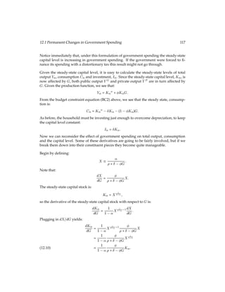
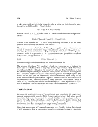
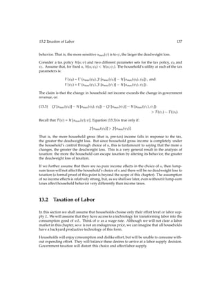
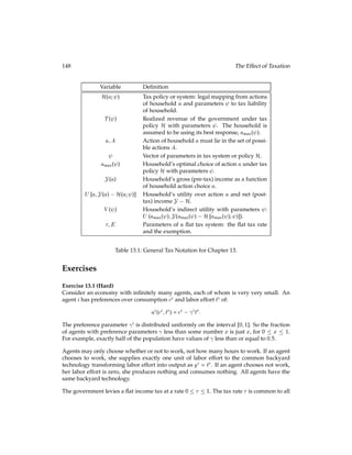
295. 13.1 General Analysis of Taxation 133
to the tax system are = fE;g and H(a; ) is:
H(a; ) =
0; a E
(a E); a E:
Definitions
We can use our notation to make some useful definitions. The marginal tax rate is the tax
paid on the next increment of a. So if one’s house had 10 windows already and one were
considering installing an 11th window, the marginal tax rate would be the increase in one’s
tax bill arising from that 11th window. More formally, the marginal tax rate at a is:
@H(a; )
@a :
Here we are assuming that a is a scalar and smooth enough so that H(a; ) is at least
once continuously differentiable. Expanding the definition to cases in which H(a; ) is
not smooth in a (in certain regions) is straightforward, but for simplicity, we ignore that
possibility for now.
The average tax rate at a is defined as:
H(a; )
a :
Note that a flat tax with E = 0 has a constant marginal tax rate of , which is just equal to
the average tax rate.
If we take a to be income, then we say that a tax system is progressive if it exhibits an
increasing marginal tax rate, that is if H0(a; ) 0. In the same way, a tax system is said to
be regressive if H0(a; ) 0.
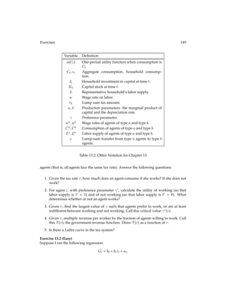
Household Behavior
Let us now turn our attention to the household. The household has some technology for
producing income Y1
that may be a function of the action a, so Y(a). If a is hours worked,
then Y is increasing in a, if a is hours of leisure, then Y is decreasing in aand if ais house-
windows then Y is not affected by a. The household will have preferences directly over
action a and income net of taxation Y(a) H(a; ). Thus preferences are:
U [a;Y(a) H(a; )] :
There is an obvious maximization problem here, and one that will drive all of the analysis
in this chapter. As the household considers various choices of a (windows, hours, yachts),
1We use the notation Y here to mean income to emphasize that income is now a function of choices a.

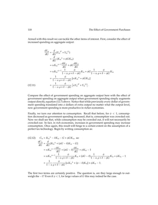
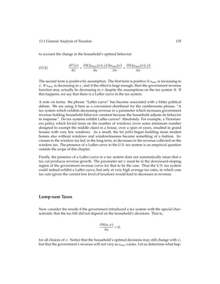
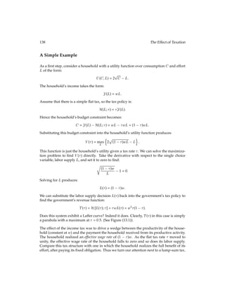
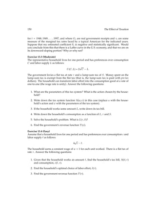
296. 134 The Effect of Taxation
it takes into consideration both the direct effect of a on utility and the indirect effect of a,
through the tax bill term Y(a) H(a; ). Define:
V( ) max
a2A
U [a;Y(a) H(a; )] :
For each value of , let amax( ) be the choice of awhich solves this maximization problem.
That is:
V( ) = U [amax( );Y(amax( )] H[amax( ); )] :
Assume for the moment that U, Y and H satisfy regularity conditions so that for every
possible jpsithere is only one possible value for amax.
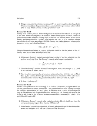
The government must take the household’s response amax( ) as given. Given some tax
system H, how much revenue does the government raise? Clearly, just H[amax( ); ]. As-
sume that the government is aware of the household’s best response, amax( ), to the gov-
ernment’s choice of tax parameter . Let T ( ) be the revenue the government raises from
a choice of tax policy parameters :
T ( ) = H[amax( ); ]:
(13.1)
Notice that the government’s revenue is just the household’s tax bill.
The functions H(a; ) and T ( ) are closely related, but you should not be confused by
them. H(a; ) is the tax system or tax policy: it is the legal structure which determines
what a household’s tax bill is, given that household’s behavior. Households choose a value
for a, but the tax policy must give the tax bill for all possible choices of a, including those
that a household might never choose. Think of H as legislation passed by Congress. The
related function T ( ) gives the government’s actual revenues under the tax policy H(a; )
when households react optimally to the tax policy. Households choose the action a which
makes them happiest. The mapping from tax policy parameters to household choices is
called amax( ). Thus the government’s actual revenue given a choice of parameter , T ( ),
and the legislation passed by Congress, H(a; ), are related by equation (13.1) above.
The Laffer Curve
How does the function T ( ) behave? We shall spend quite a bit of time this chapter con-
sidering various possible forms for T ( ). One concept to which we shall return several
times is the Laffer curve. Assume that, if a is fixed, that H(a; ) is increasing in (for ex-
ample, could be the tax rate on house windows). Further, assume that if is fixed, that
H(a; ) is increasing in a. Our analysis would go through unchanged if we assumed just
the opposite, since these assumptions are simply naming conventions.
Given these assumptions, is T necessarily increasing in ? Consider the total derivative of
T with respect to . That is, compute the change in revenue of an increase in , taking in