Download as PDF, PPTX

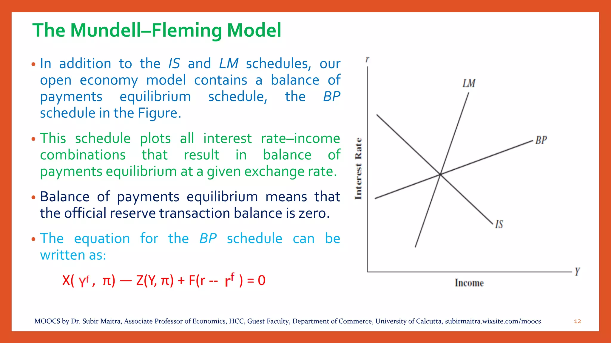
![The Mundell–Fleming Model
Exports:
• U.S. exports are other countries’ imports and thus depend positively on foreign income
( ) and the exchange rate:
X = X( , π), X > 0; > 0
• The latter relationship follows because a rise in the exchange rate lowers the cost of dollars
measured in terms of the foreign currency and makes U.S. goods cheaper to foreign
residents.
Product Market Equilibrium Condition:
• Thus, the product market equilibrium condition can be written as:
I(r) + G0 + [X( , π) — Z(Y, π)] = S(Y—T(Y)) + T(Y)
From this equation, the IS schedule is obtained for the open economy.
8MOOCS by Dr. Subir Maitra, Associate Professor of Economics, HCC, Guest Faculty, Department of Commerce, University of Calcutta, subirmaitra.wixsite.com/moocs](https://image.slidesharecdn.com/is-lmmodel5-180708172003/75/IS-LM-Model-5-8-2048.jpg)
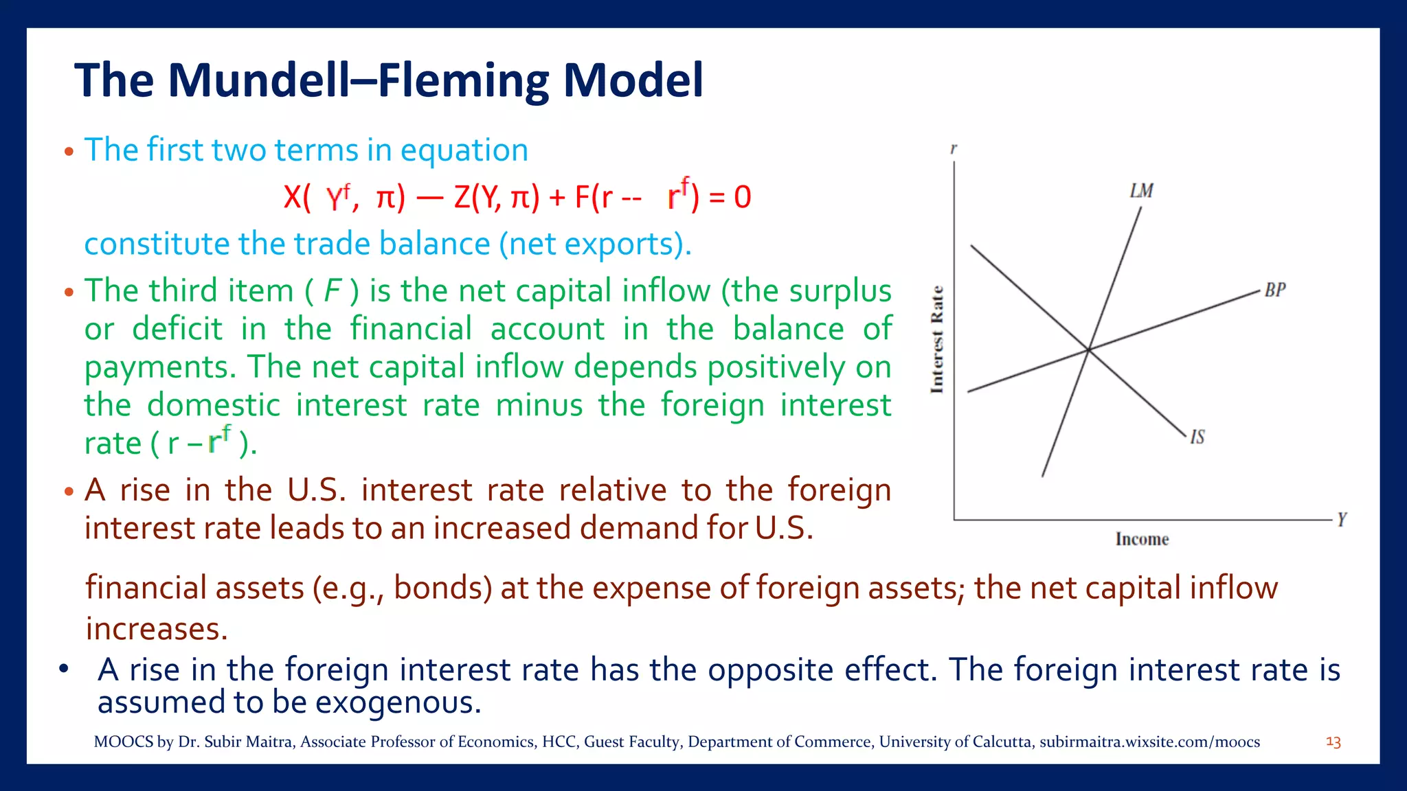
![The Mundell–Fleming Model
• High values of the interest rate will result in low levels
of investment. To satisfy equation
I(r) + G0 + [X( , π) — Z(Y, π)] = S(Y—T(Y)) + T(Y)
at such high levels of the interest rate, income must
be low so that the levels of imports and saving will be
low.
▪ Alternatively, at low levels of the interest rate, which
The open economy IS schedule is also downward sloping, as shown in the Figure.
result in high levels of investment, goods market equilibrium requires that saving and
imports must be high; therefore, Y, must be high.
9MOOCS by Dr. Subir Maitra, Associate Professor of Economics, HCC, Guest Faculty, Department of Commerce, University of Calcutta, subirmaitra.wixsite.com/moocs](https://image.slidesharecdn.com/is-lmmodel5-180708172003/75/IS-LM-Model-5-9-2048.jpg)
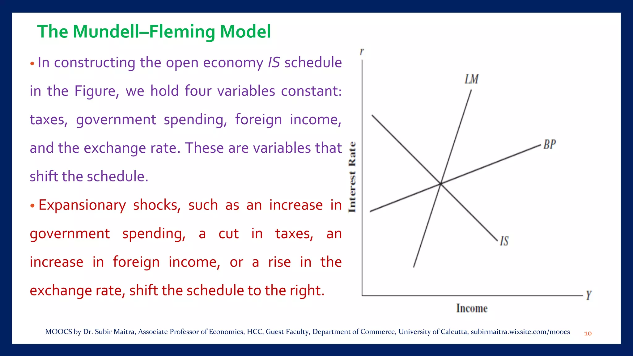
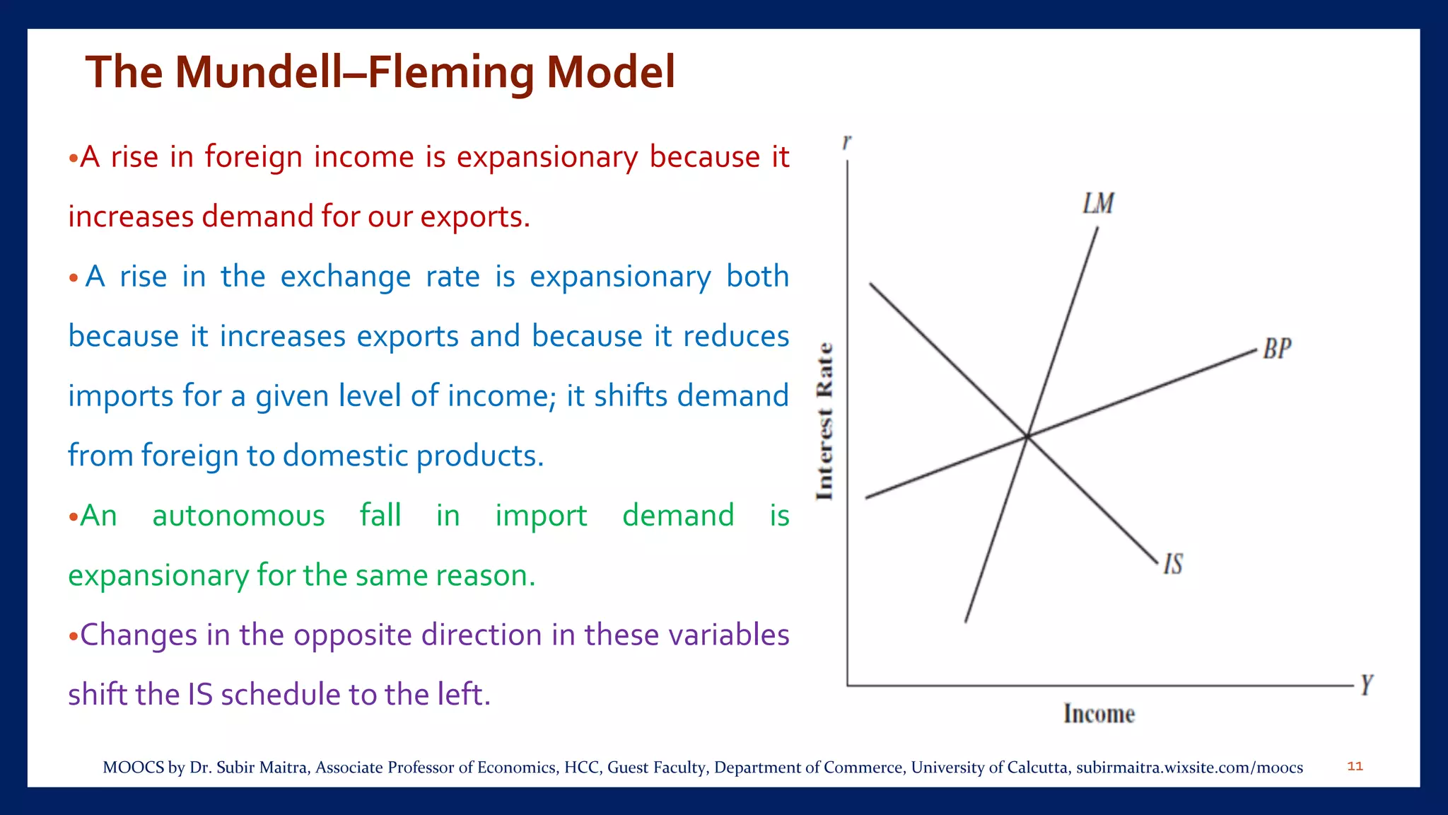


The document discusses the Mundell-Fleming model of an open economy. It introduces the IS-LM model and describes how the Mundell-Fleming model incorporates international trade and capital flows. Specifically, it adds an exports and imports term to the goods market equilibrium equation and a capital flows term to the balance of payments equation. The model includes downward-sloping IS and LM curves and an upward-sloping BP curve. It analyzes the effects of monetary and fiscal policy under fixed exchange rates, finding that expansionary monetary policy leads to a balance of payments deficit while fiscal policy can result in either a surplus or deficit.