Advanced Lane Finding

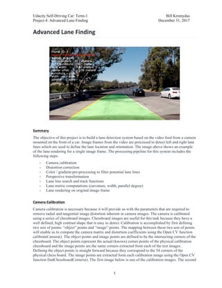
Udacity Self-Driving Car: Term-1 Bill Kromydas
Project 4: Advanced Lane Finding December 31, 2017

1
Advanced Lane Finding

Summary
The objective of this project is to build a lane detection system based on the video feed from a camera
mounted on the front of a car. Image frames from the video are processed to detect left and right lane
lines which are used to define the lane location and orientation. The image above shows an example
of the lane rendering for a single image frame. The processing pipeline for this system includes the
following steps:
- Camera calibration
- Distortion correction
- Color / gradient pre-processing to filter potential lane lines
- Perspective transformation
- Lane line search and track functions
- Lane metric computations (curvature, width, parallel degree)
- Lane rendering on original image frame

Camera Calibration
Camera calibration is necessary because it will provide us with the parameters that are required to
remove radial and tangential image distortion inherent in camera images. The camera is calibrated
using a series of chessboard images. Chessboard images are useful for this task because they have a
well defined, high contrast shape that is easy to detect. Calibration is accomplished by first defining
two sets of points: “object” points and “image” points. The mapping between these two sets of points
will enable us to compute the camera matrix and distortion coefficients using the Open CV function
calibrateCamera(). The object points and image points are defined to be the intersecting corners of the
chessboard. The object points represent the actual (known) corner points of the physical calibration
chessboard and the image points are the same corners extracted from each of the test images.
Defining the object points is straight forward because they correspond to the 54 corners of the
physical chess board. The image points are extracted form each calibration image using the Open CV
function findChessboardCorners(). The first image below is one of the calibration images. The second


2
image shows the identified image points that were detected using findChessboardCorners(). The last
image is the undistorted image that was transformed using the camera matrix and distortion
coefficients. Each calibration image can be used to compute a camera matrix and the distortion
coefficients. Once these are computed for each calibration image they can be averaged across all
calibration images to compute a final camera matrix and the associated distortion coefficients for the
camera. Once the camera is calibrated these parameters can be used to undistorted the images from
the video frames prior to image processing.
calibration image corner detection undistorted image
Perspective Transform
Perspective transformations be very useful for transforming images into a space that is easier to work
with. Consider the camera image below to the left. If we transform that image to a bird’s eye view
from above then the computations for lane curvature and other metrics will be greatly simplified and
easier to visualize. This perspective is also helpful for comparing a car’s location directly with a map.
In order to define a bird’s eye view perspective transformation we need to define a rectangle on a
plane in the original image. We will call these points “source” points. They define the points of
interest in the original image that lie in a plane in the physical world. Next we need to map those
points to a set of four destination points in a warped image. Once we have defined both sets of points
we can use the Open CV function getPerspectiveTransform() to compute the perspective
transformation matrix (and its inverse). Once we have the transformation matrix (M) we can use the
Open CV function warpPerspective() to transform an image to a bird’s eye view perspective. The
source and destination points that I selected are listed in the table below.
Source points Destination Points
x y x y
567 470 314 0
720 470 986 0
1100 720 986 720
205 720 314 720
The examples below show the undistorted camera image to the left with a red trapezoid that defines a
“rectangular” region on the road surface. We assume the road is flat and that the lane lines in these
images are parallel which allow us to define the source points that represent a rectangle in real word
space. The images to the right show the transformed (warped) image as a bird’s eye view with the
expected result (i.e., the trapezoid is now transformed to a rectangle in the warped image). See
get_src_dst_points() in lane_line_helpers.py. For the selected source and destination points the lane
width in pixel space is about 690 pixels. This calibrated value will be used to estimate the lane width
when processing images. It is important to select the source points so the top of the trapezoid is high
enough in the image frame to capture lane line detections close to the road horizon. This allows the


3
system to detect lane curvature sooner near the horizon and also maximizes the opportunity for
detecting an adequate number of “dashed” line segments which is important for a robust curve fit.

Image Filtering

In order to detect lane lines from camera images two thresholding approaches were recommended in
the lecture notes (color filtering and gradient filtering). Assuming all lane lines are either yellow or
white as in all the test images and videos, I looked for color channels in various color spaces that
might perform well for detecting either of these colors under various lighting conditions. The images
on the following page show some of the better color channels for detecting yellow and white lane
lines. I considered four color spaces: RGB, HLS, LAB and HSV and experimented with each of the
channels across a range of images. There are a number of channels that appear to perform equally
well for detecting white (RGB, HSV-V, LAB-L). However, LAB-B stands out as the best channel for
detecting yellow, especially in low light conditions.
I also experimented with gradient thresholds as recommended in the lecture notes but I found that
color thresholding seemed to be the dominate factor. For gradients, I used Sobel-x as well as gradient
magnitude and direction. I was able to reproduce (almost exactly) the binary filtered image for
test5.jpg as shown in the lecture notes using a combined color and gradient filter with an OR
operation between color and gradients.
combined_binary[(color_binary == 1) | (grad_binary == 1)] = 1
This filter performed well for detecting many lane lines with nice precision, but it failed for cases in
the challenge video where seams in the road surface could not be masked due to the strong gradient
and linear nature of such features. I therefore opted to use an AND operation with different threshold
values for combining color and gradients to minimize false detections due to gradients.
combined_binary[(color_binary == 1) & (grad_binary == 1)] = 1


4

undistorted image undistorted image

LAB-B Channel LAB-B Channel

HSV-V Channel HSV-V Channel

RGB-R Channel RGB-R Channel

LAB-L Channel LAB-L Channel


5
Image Pre-Processing
The two sets of four images below illustrate the effect of combining color and gradient with an AND
operation between them in the final filtered image (lower right in each quadrant). In the first set of
images either color or gradient alone would have been adequate for lane detection. However, in the
second set of images it is clear that the combined filter does the best job at eliminating clutter.
undistorted image color filter only
gradient filter only combined (color & gradient)
undistorted image color filter only
gradient filter only combined (color & gradient)


6
Processing Pipeline
The processing pipeline for lane detection consists of the following steps:
- image un-distortion
- image filtering (color and gradient)
- image warping
- image region of interest clipping
- lane acquisition via sliding window search
- lane tracking via band search for previously detected lanes
- polynomial fitting to the detected line points
- computation of lane line metrics (curvature, width, parallel)
- final lane rendering on original image
The following images illustrate the key processing steps in the pipeline.

undistorted image color and gradient filtered

binary warped image (clipped) sliding window search

polynomial fit tracking final lane rendering projected on original image


7
Search Modes
I experimented with the sliding window search mode and the convolution centroid approach. I found
the sliding window search mode to be more robust at identifying lane lines and I therefore focused on
that implementation for this project. I used 18 sliding windows with a pixel margin of +/- 80 pixels.
This seemed to provide a good resolution for initial detection of lane lines. In order to minimize the
effect of clutter from the center of the lane I created a keep-out zone so the histogram computation for
computing the peaks ignores the keep-out region in the center of the lane. I also made a configurable
parameter (HIST_FRACTION = .8) that allows the histogram to examine data through a greater
portion of the image frame (i.e., greater than the lower half). This is useful for acquiring lane
detections when there is no detectable data in the lower half of the image frame.
Lane Tracking
Once the lane has been detected using the sliding window search mode it is maintained in a track
mode which uses a search band around the best fit polynomial for each lane line. The best fit
polynomial is computed as the running average of the last N image frames which helps to smooth the
transition from frame to frame (N_FRAMES_SMOOTH = 3). The search band in the current frame is
defined by the best fit polynomial from previous frames. The search band is used to find new line
detections which are used to compute a new current polynomial fit. If a given frame has no detections
or does not pass the lane metric criteria for lane detection then the current frame is skipped and the
previous best fit polynomials are used to render the lane in the original image. The number of
consecutive frames that can be skipped in track mode before the sliding window search mode is
executed is a configurable parameter (MAX_FRAMES_SKIPPED = 5).
Lane Metrics
Both search and track modes described above use a final confirmation step to determine if the lane
has been detected. The confirmation step uses three separate metrics: (1) minimum lane curvature, (2)
lane width, (3) parallel lane lines. Each of these metrics must be satisfied within configurable
threshold limits in order to declare the lane detected. The lane line curvature of both lane lines must
be greater than a minimum configurable threshold. The lane width is measures at the base of the
image frame and must be within a +/- threshold value to the standard lane width of 3.7 meters.
Parallel lines are checked by comparing the first two coefficients (quadratic and liner terms) of each
polynomial fit to threshold values to check for their similarity.

Examples
The series of images on the following page show two of the more challenging image frames. The
image on the left is challenging due to the white colored pavement and an abundance of clutter which
both compete with detecting the lane lines. In spite of the relatively poor quality of the filtered image
the sliding window search method does a good job of identifying the lane lines. The image on the
right shows the car emerging from the shadow of the bridge. In this case the system lost track of the
lane lines while under the bridge and was attempting to reacquire the lines using a sliding window
search. Rather than using only the bottom half of the image frame to compute the histogram peaks I
made that a configurable parameter so that situations like this could be handled by allowing the
algorithm to use more of the data in the upper portion of the image frame to kick start the detection
process sooner. I also added a keep out zone in the center of the image which is also configurable.
The purpose of the keep-out zone is to mask clutter in the center of the lane from the peak histogram
computations so that the clutter does cause false lane line detections.


8


9
Lane Rendering and Diagnostics
For each image frame the detected lane is rendered on the original image as a transparent green swath
between the two polynomial lane line fits. The left and right lane boundaries are outline in yellow.
Several diagnostics are displayed in the upper left portion of the frame to identify the status of the
lane detection which is very useful for debugging.

Reflection
This project presented an opportunity to solve an interesting and challenging problem using a wide
range of methods. In retrospect I would have spent more time up-front investigating more robust
methods for image filtering and creating diagnostics to improve the experimentation process. The
main thing I would spend more time exploring would be adaptive thresholding techniques. All of the
color and gradient thresholding I implemented for this project consisted of fixed threshold values
which can work in some cases and not in others. Manually tuning threshold parameters is tedious to
begin with and is not robust due to fixed values. I believe an adaptive thresholding technique that
depends on the local conditions (lighting, texture, etc…) would have been a much more robust
approach. Other image processing techniques may have also worked better to isolate the lane lines. I
experimented with a technique to clone a lane line when the detections from one line were
significantly unbalance compared to the other line. This proved to be only marginally useful in the
current implementation and sometimes buggy, so it was not included in the default configuration. I
also did not make use of the lane center offset that was computed. This information could be used to
dynamically adjust the lane detection and tracking functions.


10

Files Submitted
This project includes the following source files:
Files Description
lane_finder_driver.py Test driver
camera_calibration.py Camera calibration
image_pipeline.py Main processing routine for each image
filter_lane_lines.py Filter images
lane_line_helpers.py Convenience functions
find_lines_from_sliding_window.py Sliding window search algorithm
find_lines_from_fit.py Lane tracking algorithm
Line.py Line class
Lane.py Lane class
params.py Tuning parameters

Default Tuning Parameters
MAX_FRAMES_SKIPPED = 5 # max number of skipped frames before sliding window
search must be performed
N_FRAMES_SMOOTH = 3 # number of image frames to smooth

MIN_CURVATURE_METERS = 350 # tightest lane curvature allowed for an individual frame

NUM_SLIDING_WINDOWS = 18 # number of (vertically stacked) sliding windows
MIN_WINDOW_PIX = 20 # min number of pixels in a window to trigger a detection
CENTER_KEEPOUT = 100 # ignore keep-out region in center of image frame
HIST_FRACTION = .8 # percentage of frame (from bottom) to use for histogram
WINDOW_MARGIN = 80 # sliding window margin (+/- width) for detections
FIT_MARGIN = 60 # pixel margin around fitted lane line
LANE_WIDTH_PIX = 690 # from calibrated strait line image (base of image frame)
LANE_WIDTH_METERS = 3.7 # standard (actual) distance between lane lines
LANE_WIDTH_MARGIN = .9 # lane width margin threshold

SOBEL_KERNEL = 9

LANE_WIDTH_TRESH = (LANE_WIDTH_METERS - LANE_WIDTH_MARGIN, LANE_WIDTH_METERS +
LANE_WIDTH_MARGIN)

PARALLEL_THRESH = (0.0005, # squared term
0.09) # linear term

FILTER_GRADIENT = 'all' # = 'all', combine sobel-x and (dir, mag), otherwise just sobel-x
FILTER_COMBINED = 'all' # = 'all', combine color and gradient above, otherwise just color

YM_PER_PIX = 30/720 # meters per pixel in y dimension
XM_PER_PIX = LANE_WIDTH_METERS/LANE_WIDTH_PIX # meters per pixel in x dimension

Advanced Lane Finding

Recommended

Recommended

More Related Content

What's hot

What's hot (20)

Similar to Advanced Lane Finding

Similar to Advanced Lane Finding (20)

Recently uploaded

Recently uploaded (20)

Advanced Lane Finding