Econometrics1,2,3,4,5,6,7,8_ChaptersALL.pdf

Temesgen Keno (Ph.D.)
Asst. Prof. of Development Economics
College of Business and Economics
Haramaya University
Introduction to Econometrics
(MBA 525)
1

Chapter 1: Introduction
This chapter discusses
 Definition and scope of econometrics
 Need, objectives and goal of econometrics
 Economic vs. econometric models
 Methodology of econometrics
 Desirable properties of econometric models
 Data structures in econometric analysis
 Causality and the notion of ceteris paribus
2

 The course Introduction to Econometrics
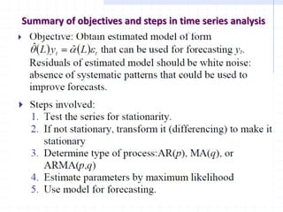
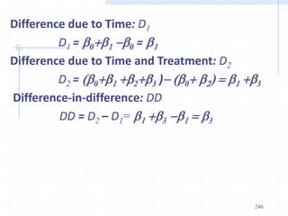
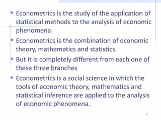
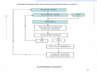
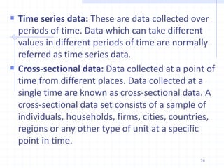
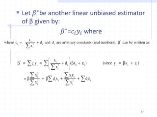
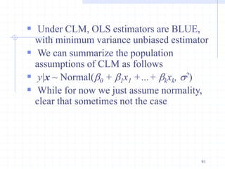
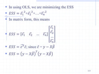
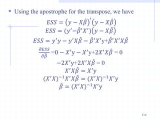
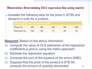
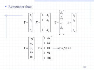
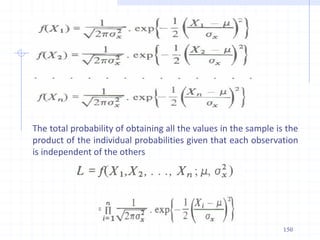
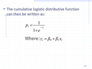
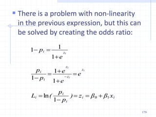
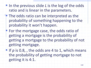
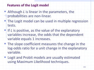
provides a comprehensive introduction to the
art and science of econometrics.
 It deals with how theory, statistical and
mathematical methods are combined in the
analysis of business and economics data, with
a purpose of giving empirical content to the
theories, and then verify or refute them.
3

1.1 Definition and scope of econometrics
 Data analysis in economics, finance, marketing,
management and other disciplines is increasingly
becoming quantitative.
 This involves estimation of parameters or
functions, quantification of qualitative
information and making hypotheses.
 Developing the quantitative relationships among
various economic variables is important to better
understand the relationships, and to provide
better guidance for economic policy making.
4

 What is econometrics? Literally, econometrics
means “economic measurement”, but its scope
is much broader.
 Derived from the Greek terms ‘Oikovomia’
which means economy, and ‘Metopov’ which
means measurement.
 “Econometrics is the science which integrates
economic theory, economic statistics, and
mathematical economics to investigate the
empirical support of the general schematic law
established by economic theory.
.
5

 Econometrics is a special type of economic
analysis and research in which the general
economic theories, formulated in mathematical
terms, are combined with empirical
measurements of economic phenomena.
 Econometrics is defined as the quantitative
analysis of actual economic phenomena.
 Econometrics is the systematic study of
economic phenomena using observed data.
6

 Econometrics is the study of the application of
statistical methods to the analysis of economic
phenomena.
 Econometrics is the combination of economic
theory, mathematics and statistics.
 But it is completely different from each one of
these three branches
 Econometrics is a social science in which the
tools of economic theory, mathematics and
statistical inference are applied to the analysis
of economic phenomena.
7

 Econometrics may be considered as the
integration of economics, mathematics and
statistics for the purpose of providing
numerical values for the parameters of
economic relationships.
 Econometric methods are statistical methods
specifically adapted to the peculiarities of
economic phenomena.
 The most important characteristic of
economic relationships is that they contain a
random element.
8

 However, such random element is not
considered by economic theory and
mathematical economics which postulate
relationship between the various economic
magnitudes
 Econometrics is the science of testing economic
theories.
 Econometrics is the set of tools used for
forecasting the future values of economic
variables.
9

 Econometrics is the process of fitting
mathematical economic models to real world
data.
 Econometrics is the science and art of using
historical data to make numerical or
quantitative analysis for policy
recommendations in government and business
 Econometrics is the science and art of using
economic theory and statistical techniques to
analyze economic data.
10

1.2. Need, objectives and goal of econometrics
A. The Need for Econometrics
 Econometrics is fundamental for economic
measurement.
 However, its importance extends far beyond the
discipline of economics.
 Econometrics has three major uses;
1. Describing economic reality
 The simplest use of econometrics is description
 We can use econometrics to quantify economic
activity b/c econometrics allows us to estimate
numbers and put them in equations that
previously contained only abstract symbols.
11

2. Testing hypotheses about economic theory
The second and perhaps the most common use
of econometrics is hypothesis testing, the
evaluation of alternative theories with
quantitative evidence
 Much of economics involves building theoretical
models and testing them against evidence, and
hypothesis testing is vital to that of scientific
approach.
12

3. Forecasting future economic activity
 The third and most difficult use of
econometrics is to forecast or predict what is
likely to happen in the future based on what
has happened in the past.
 Economists use econometric models to make
forecasts of variables like sales, profits, gross
domestic products (GDP), and inflation.
13

B. The goals of econometrics
 Three main goals of econometrics are often
identified, including
1. Analysis (i.e., testing economic theory).
2. Policy making (i.e., obtaining numerical
estimates of the coefficients of economic
relationships for policy simulations, and
3. Forecasting (i.e., using the numerical estimates
of the coefficients in order to forecast the
future values of economic magnitudes.
14

1.3 Economic vs. Econometric Models
 Economic models: Any economic theory is an
observation from the real world.
― For one reason, the immense complexity of the
real world economy makes it impossible to
understand all interrelationships at once.
― Another reason is that all the interrelationships
are not equally important as such for the
understanding of the economic phenomenon
under study.
15

 The sensible procedure is therefore, to pick
up the important factors and relationships
relevant to our problem and to focus our
attention on these alone.
 Such a deliberately simplified analytical
framework is called on economic model.
 It is an organized set of relationships that
describes the functioning of an economic
entity under a set of simplifying
assumptions.
16

 All economic reasoning is ultimately based on
models.
 Economic models consist of the following
three basic structural elements;
 A set of variables
 A list of fundamental relationships and
 A number of strategic coefficients or
parameters
17

 Econometric models: As their most important
characteristic, economic relationships contain
a random element which is ignored by
mathematical economic models which
postulate exact relationships between
economic variables.
 Example: Economic theory postulates that the
demand for a commodity depends on its
price, on the prices of other related
commodities, on consumers’ income and on
tastes.
18

 This is an exact relationship which can be
written mathematically as:
 The above demand equation is exact.
 However, many more factors may affect
demand. In econometrics the influence of
these ‘other’ factors is taken into account by
the introduction into the economic
relationships of random variable.
T
b
Y
b
P
b
P
b
b
Q o 4
3
2
1
0 




19

 In our example, the demand function
studied with the tools of econometrics
would be of the stochastic form:
 Where i stands for the random factors
which affect the quantity demanded
including.
i
T
b
Y
b
P
b
P
b
b
Q ε





 4
3
0
2
1
0
20

Causes of the error
 Omission of variables from the
function
 Random behaviour of human beings
 Imperfect specification of the
mathematical form of the model
 Errors of aggregation
 Errors of measurement
21

1.4. Methodology of econometrics
The general methodological approaches in
econometrics include:
 Specification of the model
 Estimation of the model
 Evaluation of the estimates
 Evaluation of the forecasting power of
the model
22

The elements or anatomy of the set up that
constitute an economic analysis thus
involves:
 Economic Theory
 Mathematical Model of Theory
 Econometric Model of Theory
 Data
 Estimation of Econometric Model
 Hypothesis Testing
 Forecasting or Prediction
 Using the model for control or policy
purposes
23

Fig: Methodologies of econometrics
24

1.5. Desirable properties of Econometric
Models
 Theoretical plausibility
 Explanatory ability
 Accuracy of the estimates of the parameters
 Forecasting ability
 Simplicity
25

1.6. Data structures in econometrics analysis
 The success of any econometric analysis ultimately
depends on the availability of the appropriate data.
 It is therefore essential that we spend some time discussing
the nature, sources, and limitations of the data that one
may encounter in empirical analysis.
Sources and Types of Data
 In econometrics, data come from two sources: experiments
or non-experiment observations.
 Experimental data come from experiments designed to
evaluate a treatment or policy to investigate a casual effect.
 Non-experimental data are data obtained by observing
actual behavior outside an experimental setting.
26

 It is also known as observational data
 Observational data are collected using surveys
such as personal interview or telephone interview
or any other methods of collecting primary data.
 Observational data pose major challenges to
econometric attempts to estimate casual effects.
 Whether data are experimental or observational,
data sets come in three main types: Time series,
cross-sectional and pooled data.
 Data can be available for empirical analysis in the
form of time series, cross-section, pooled and
panel data
27

 Time series data: These are data collected over
periods of time. Data which can take different
values in different periods of time are normally
referred as time series data.
 Cross-sectional data: Data collected at a point of
time from different places. Data collected at a
single time are known as cross-sectional data. A
cross-sectional data set consists of a sample of
individuals, households, firms, cities, countries,
regions or any other type of unit at a specific
point in time.
28

 Pooled data: Data collected over periods of
time from different places. It is the
combination of both time series and cross-
sectional data.
 Panel data: It is also known as longitudinal
data. It is a time series data collected from
the same sample over periods of time.
29

1.7. Causality and the notion of ceteris paribus
 Simply establishing a relationship between
variables is rarely sufficient
 Effects are required to be considered causal
 If we’ve truly controlled for enough other
variables, then the estimated ceteris paribus
effect can often be considered to be causal
 Otherwise, it can be difficult to establish
causality.
30

 The concept of ceteris paribus, that is holding
all other factors constant, is at the center of
establishing a casual relationship.
 Simply finding that two variables are
correlated is rarely enough to conclude that a
change in one variable causes a change in
another.
 The goal of most empirical studies in
economics and other social sciences is to
determine whether a change in one variable,
say x, causes a change in the other variable,
say y.
31

 For example, does having another year of
education cause an increase in monthly salary?
 Does reducing class size cause an
improvement in student performance?
 Because economic variables are properly
interpreted as random variables, we should
use ideas from probability to formalize the
sense in which a change in x causes a change
in y.
32

Example: Returns to Education
 A model of human capital investment implies getting
more education should lead to higher income/earnings
 In the simplest case, this implies an equation like
 The estimate of b1, is the return to education, but can it
be considered causal?
 While the error term, , includes other factors affecting
earnings, so that we need to control for as much as
possible
 Some things are still unobserved, which can be
problematic.
ε
β
β 

 Education
Earning 1
0
33

Chapter 2: Simple Linear Regression Model
 Introduction to two-variables linear regression
 Assumptions of the classical linear regression
model
 The ordinary least squares (OLS) method of
estimation
 The Guass-Markov Theorem
 Statistical Inference in simple linear regression
model
 Tests of model adequacy
 Tests of significance of OLS parameters
34

2.1. Introduction
 Simple Linear Regression Model is a classical
linear regression model for examining the nature
and form of the relationships between two
variables.
 It involves only two variables (so called SLRM) as
compared to multiple linear regression which
involves k- variables.
 Regression analysis is a statistical method that
attempts to explain movements in one variable,
the dependent variable, as a function of
movements in a set of other variables, called
independent variables. 35

 Regression analysis is concerned with describing and
evaluating the relationship between a given variable
(often called the dependent variable) and one or
more variables which are assumed to influence the
given variable (often called independent or
explanatory variables).
 The simplest economic relationship is represented
through a two-variable model (also called the simple
linear regression model) which is given by:
Y= a + bX
where a and b are unknown parameters (also called
regression coefficients) that we estimate using
sample data. Here Y is the dependent variable and X
is the independent variable. 36

 Example: Suppose the relationship between
expenditure (Y) and income (X) of households is
expressed as:
Y= 120 + 0.6X
 Here, on the basis of income, we can predict
expenditure. For instance, if the income of a certain
household is 1500 Birr, then the estimated
expenditure will be: expenditure = 0.6(1500) + 120 =
1020 Birr
 Note that since expenditure is estimated on the
basis of income, expenditure is the dependent
variable and income is the independent variable.
37

Error term
 Consider the above model: Y = 0.6X + 120.
 This functional relationship is deterministic or exact,
that is, given income we can determine the exact
expenditure of a household.
 But in reality this rarely happens: different
households with the same income are not expected
to spend equal amounts due to habit persistence,
geographical and time variation, etc.
 Thus, we should express the regression model as:
where i is the random error term (also called
disturbance term).
i
i
i ε
βX
α
Y 


38

General reasons for the error term
 Omitted variables: a model is a simplification of
reality.
 It is not always possible to include all relevant
variables in a functional form.
 For instance, we may construct a model relating
demand and price of a commodity.
 But demand is influenced not only by own price:
income of consumers, price of substitutes and several
other variables also influence it.
 The omission of these variables from the model
introduces an error.
 Measurement error: Inaccuracy in collection and
measurement of sample data. 39

 Sampling error: Consider a model relating
consumption (Y) with income (X) of households.
 Poor households constitute the sample.
 Our α and β estimation may not be as good as that
from a balanced sample group.
 The size of the error i is not fixed, it is non-
deterministic or stochastic or probabilistic in nature.
 This implies that Yi is also probabilistic in nature.
 Thus, the probability distribution of Yi and its
characteristics are determined by the values of Xi and
by the probability distribution of i
40

 Thus, a full specification of a regression model should
include a specification of the probability distribution
of the disturbance (error) term. This information is
given by what we call basic assumptions or
assumptions of the classical linear regression model
(CLRM).
 Consider the model:
Yi = a + bXi+ i;… i=1,2,…n
Here the subscript i refers to the i-th observation. In
the CLRM, Yi and Xi are observable while i is not. If i
refers to some point or period of time, then we speak
of time series data. On the other hand, if i refers to
the i-th individual, object, geographical region, etc.,
then we speak of cross-sectional data.
41

2.2. Assumptions of the CLRM
1. The true model is: Yi = a + bXi+ i whereas a is the
intercept and b is the slope parameter, and i is the
error term, stochastic term (or disturbance)
2. The error terms have zero mean: E(i ) = 0. This is
often called the zero conditional mean assumption.
3. Homoscedasticity (error terms have constant
variance): Var (i ) = E(i
2 ) = s2
4. No error autocorrelation (the error terms i are
statistically independent of each other): cov (i, j) =
E(ij) = 0; for all i ≠ j .
5. Xi are deterministic (non-stochastic): Xi and i are
independent for all i, j
6. Normality: i are normally distributed with mean zero
and variance s2 for all i (written as: i ∼ N(0 , s2). 42

Let us examine the meaning of these assumptions:
 Assumption (1) states that the relationship between Yi
and Xi is linear, and that the deterministic component
(α + βXi ) and the stochastic component (i ) are
additive.
 The model is linear in parameters and I is a random
real number.
 Assumption (2) tells us that the mean of the Yi is:
E(Yi) = α + βXi
This simply means that the mean value of Yi is non-
stochastic.
 Assumption (3) tells us that every disturbance has the
same variance s2 whose value is unknown, that is,
regardless of whether the Xi are large or small, the
dispersion of the disturbances is the same.
43

 For example, the variation in consumption level of
low income households is the same as that of high
income households.
 Assumption (4) states that the disturbances are
uncorrelated. For example, the fact that output is
higher than expected today should not lead to a higher
(or lower) than expected output tomorrow.
 Assumption (5) states that Xi are not random
variables, and that the probability distribution of i is
in no way affected by the Xi .
44

 We need assumption (6) for parameter estimation
purposes and also to make inferences on the basis of
the normal (t and F) distribution.
 Specifying the model and stating its underlying
assumptions are the first stage of any econometric
application.
 The next step is the estimation of the numerical values
of the parameters of economic relationships.
 The parameters of the simple linear regression model
can be estimated by various methods.
45

2.3. The ordinary least squares (OLS)
method of estimation
 Three of the most commonly used methods
are:
1. Ordinary Least Square (OLS) method
2. Maximum Likelihood (MLM) Method
3. Method of Moments (MM) method
 But, here we will deal with the OLS and
the MLM methods of estimation.
46

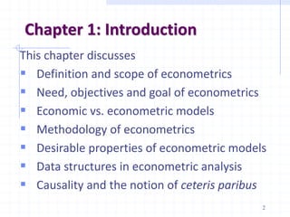
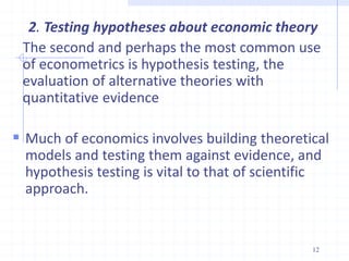
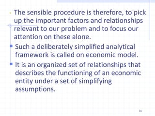
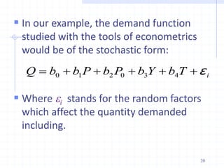
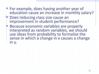
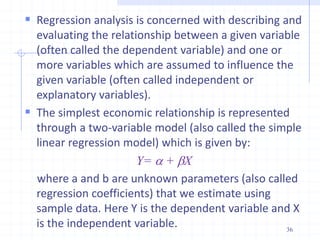
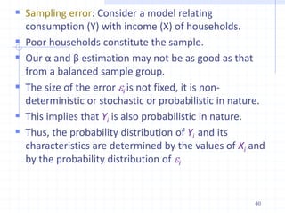
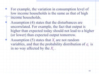
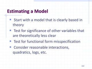
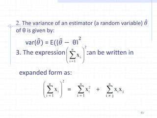
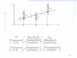
2.3. The ordinary least squares (OLS) method of
estimation
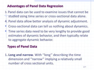
 In the regression model Yi = a + bXi+ i , the values of
the parameters α and β are not known. When they
are estimated from a sample of size n, we obtain the
sample regression line given by:
where α and β are estimated by and respectively,
and is the estimated value of Y.
 The dominating and powerful estimation method of
the parameters (or regression coefficients) α and β is
the method of least squares. The deviations between
the observed and estimated values of Y are called the
residuals, . [Note 1: Proof]
,...n
,
,i
X
β
α
Y i
i 2
1


 ˆ
ˆ
ˆ
α
ˆ β
ˆ
Y
ˆ
ε
ˆ 47

2.4. The Guass-Markov Theorem
 Under assumptions (1) – (5) of the CLRM, the OLS
estimators 𝛼 and 𝛽 are Best Linear Unbiased
Estimators (BLUE).
 The theorem tells us that of all estimators of α and β
which are linear and which are unbiased, the
estimators resulting from OLS have the minimum
variance, that is, estimators 𝛼 and 𝛽 are the best
(most efficient) linear unbiased estimators (BLUE) of α
and β.
 Note: If some of the assumptions stated above do not
hold, then OLS estimators are no more BLUE!!!
48

Proofing the theorem
 Here we will proof 𝛽 is the BLUE of β.
a) To show that 𝜷 is the a linear estimator of β
The OLS estimator of β can be expressed as
Thus, we can see that proof 𝛽 is a linear
estimator as it can be written as a weighted
average of the individual observations on 𝑦𝑖
49

b). To show that 𝛽 is unbiased estimator of β
 Note: An estimator of 𝜃 of 𝜃 is said to be
unbiased if: E(𝜃) = 𝜃
 Consider the model in deviations form:
Yi = bXi+ i
 Now, we have
E(b) = b (since b is a constant).
50

51
 Since 𝑋𝑖 is non-stochastic (assumption 5) and
E(i ) = 0 (assumption 2), we
 Thus,
 H
 Hence, 𝛽 is unbiased estimator of β

c) To show that 𝛽 has the smallest variance out
of all linear unbiased estimators of β
Note:
1. The OLS estimators 𝛼 and 𝛽 are calculated from a
specific sample of observations of the dependent
and independent variables.
 If we consider a different sample of
observations for Y and X, we get different values
for 𝛼 and 𝛽 are.
 This means that the values of 𝛼 and 𝛽 are may
vary from one sample to another, and hence, are
random variables.
52

2. The variance of an estimator (a random variable) 𝜃
of θ is given by:
var(𝜃) = E((𝜃 − θ)
2
3. The expression can be written in
expanded form as:
53

c). This is simply, the sum of the squares 𝑥𝑖
2
)
plus the sum of the cross product (𝑥𝑖𝑥𝑗)
 From equation (*), we have
 The variance of 𝛽 is thus can be expressed
as follows:
54

 Note that (**) follows from assumptions (3)
and (4), that is, var (𝜀𝑖) = E(𝜀𝑖
2
) = 𝛿2
for all i
and cov(𝜀𝑖,𝜀𝑗) = E(𝜀𝑖,𝜀𝑗) = 0, for all i≠ j .
Hence, Var(𝛽) =
𝛿2
𝑋𝑖
2
 We have seen above (in proof (a)) that the
OLS estimator of β can be expressed as:
56

 Let 𝛽∗
be another linear unbiased estimator
of β given by:
𝛽∗
=𝑐𝑖𝑦𝑖 where
57

To summarize,
1. β is the linear estimator of β.
2. β is the unbiased estimator of β.
3. β has the smallest variance compared to
any linear unbiased estimator.
Hence, we conclude that 𝛽 is the BLUE of β.
60

2.5. Statistical inference in simple linear regression
model
A. Estimation of standard error
 To make statistical inferences about the true
(population) regression coefficient β, we make use of
the estimator and its variance Var( ) .
 We have already seen that:
where
 Since this variance depends on the unknown
parameter, we have to estimate 𝛿2
.
 As shown above, an unbiased estimator of 𝛿2 is given
by:
B

B



xi
B
Var 2
2
δ
)
(

X
X
x i
i 

61

B. Test of model adequacy
 Is the estimated equation a useful one?
 To answer this, an objective measure of some
sort is desirable.
 The total variation in the dependent variable
Y is given by:
 Our goal is to partition this variation into
two: one that accounts for variation due to
the regression equation (explained portion)
and another that is associated with the
unexplained portion of the model.
2
)
ˆ
( Y
Y
(Y) i 

in
variation
Total
63

 
 
ESS
RSS
TSS
(ESS)
n
variatio
Residual
(RSS)
on
variati
Explained
(TSS)
Y
in
Variation
ESS
RSS
TSS
Then,
RSS
-
TSS
(ESS)
squares
of
sum
error
or
residual,
d,
unexplaine
û
)
(x
β̂
(RSS)
squares
of
sum
regression
or
explained
y
ŷ
)
(y
TSS
y
y
:
following
the
define
then
We
û
ŷ
y
part,
d
unexplaine
an
and
part,
explained
an
of
up
made
being
as
n
observatio
each
of
k
can thin
We
2
i
2
i
2
2
i
2
i
2
i
i
i
i





















64

 In other words, the total sum of squares (TSS) is
decomposed into regression (explained) sum of
squares (RSS) and error (residual or unexplained)
sum of squares (ESS)
 The total sum of squares (TSS) is a measure of
dispersion of the observed values of Y about their
mean.
 The regression (explained) sum of squares (RSS)
measures the amount of the total variability in the
observed values of Y that is accounted for by the
linear relationship between the observed values of
X and Y.
66

 The error (residual or unexplained) sum of squares
(ESS) is a measure of the dispersion of the
observed values of Y about the regression line.
 If a regression equation does a good job of
describing the relationship between two variables,
the explained sum of squares should constitute a
large proportion of the total sum of squares.
 Thus, it would be of interest to determine the
magnitude of this proportion by computing the
ratio of the explained sum of squares to the total
sum of squares.
67

 This proportion is called the sample coefficient of determination, R2
. That is Coefficient of determination (R2 ):
R2 = RSS/TSS
= 1-(ESS/TSS)
 1) The proportion of total variation in the dependent
variable (Y) that is explained by changes in the
independent variable (X) or by the regression line is equal
to: R2 *100%.
 The proportion of total variation in the dependent variable
(Y) that is due to factors other than X (for example, due to
excluded variables, chance, etc) is equal to: (1– R2)
x100%
68

Test for the coefficient of determination (R2)
 The largest value that R2 can assume is 1 (in which
case all observations fall on the regression line), and
the smallest it can assume is zero.
 A low value of R2 is an indication that
 X is a poor explanatory variable in the sense that
variation in X leaves Y unaffected, or while
 X is a relevant variable, its influence on Y is weak
as compared to some other variables that are
omitted from the regression equation, or
 The regression equation is misspecified (for
example, an exponential relationship might be
more appropriate.
69

 Thus, a small value of R2 casts doubt about the
usefulness of the regression equation.
 We do not, however, pass final judgment on the
equation until it has been subjected to an
objective statistical test.
 Such a test is accomplished by means of
analysis of variance (ANOVA) which enables
us to test the significance of R2 (i.e., the
adequacy of the linear regression model).
 The ANOVA table for simple linear regression
is given below:
70

ANOVA Table for simple Linear Regression
Source of
variation
Sum of
squares
Degree
of
freedom
Mean
square
Variance Ratio
Regression RSS 1 RSS/1
Residual ESS n-2 ESS/n-2
Total TSS n-1
2
1



n
ESS
RSS
Fcal
/
/
ESS
Sq.
Mean
RSS
Sq.
Mean
71

 To test for the significance of R2 , we compare the
variance ratio with the critical value from the F
distribution with 1 and (n-2) degrees of freedom in the
numerator and denominator, respectively, for a given
significance level α.
 Decision: If the calculated variance ratio exceeds the
tabulated value, that is, if Fcal > Fa (1,n 2) , we then
conclude that R2 is significant (or that the linear
regression model is adequate).
 The F test is designed to test the significance of all
variables or a set of variables in a regression model.
 In the two-variable model, however, it is used to test the
explanatory power of a single variable (X), and at the
same time, is equivalent to the test of significance of R2
72

Illustrative Example 1: SLR Empirics
Consider the following data on the percentage
rate of change in electricity consumption
(millions KWH) (Y) and the rate of change in
the price of electricity (Birr/KWH) (X) for the
years 1979 – 1994.
73

Year X Y Year X Y
1979 -0.13 17.93 1987 2.57 52.17
1980 0.29 14.56 1988 0.89 39.66
1981 -0.12 32.22 1989 1,80 21.80
1982 0.42 2.20 1990 7.86 -49.51
1983 0.08 54.26 1991 6.59 -25.55
1984 0.80 58.61 1992 -0.37 6.43
1985 0.24 15.13 1993 0.16 15.27
1986 -1.09 39.25 1994 0.50 60.40
Summary statistics
779.235
y
x
13228.7
Y
92.20109;
X
;
23.42688
Y
1.280625;
X
16;
n
Y
-
Y
y
and
X
-
X
x
:
Note
i
i
2
i
2
i
i
i
i
i












74

Based on the above information,
a) Compute the value of the regression
coefficients
b) Estimate the regression equation
c) Test whether the estimated regression
equation is adequate
d) Test whether the change in price of electricity
significantly affects its consumption.
75

Chapter 3
Multiple Linear Regression Models
 Introduction to k-variables linear regression
 Assumptions
 Estimation of parameters and SEs
 R-square and tests of model adequacy
 T-tests for significance of the coefficients
 Matrix forms of multiple regressions
76

3.1. Introduction
 So far we have seen the basic statistical tools
and procedures for analyzing relationships
between two variables.
 But in practice, economic models generally
contain one dependent variable and two or
more independent variables.
 Such models are called multiple linear
regression models
77

Example 1
In demand studies we study the relationship
between the demand for a good (Y) and price
of the good (X2), prices of substitute goods
(X3) and the consumer’s income (X4 ). Here,
Y is the dependent variable and X2, X3 and
X4 are the explanatory (independent)
variables. The relationship is estimated by a
multiple linear regression equation (model)
of the form:
4
4
3
3
2
2
1 X
β̂
X
β̂
X
β̂
β̂
Ŷ 



78

Example 2
In a study of the amount of output (product),
we are interested to establish a relationship
between output (Q) and labour input (L) &
capital input (K). The equations are often
estimated in log-linear form as:
)
log(
ˆ
)
log(
ˆ
ˆ
)
ˆ
log( 3
2
1 K
L
Q b
b
b 


79

Example 3
In a study of the determinants of the number
of children born per woman (Y), the possible
explanatory variables include years of
schooling of the woman (X2 ), woman’s (or
husband’s) earning at marriage (X3), age of
woman at marriage (X4) and survival
probability of children at age five (X5).
The relationship can thus be expressed as:
5
5
4
4
3
3
2
2
1
ˆ
ˆ
ˆ
ˆ
ˆ
ˆ X
X
X
X
Y b
b
b
b
b 




80

3.2. Assumptions of Multiple linear regression
1. The true model is
y = b0 + b1x1 + b2x2 + . . . bkxk + 
 b0 is still the intercept
 b1 to bk all arecalled slope parameters
  is still the error term (or disturbance)
 Still we need to make a zero conditional mean
assumption, so now assume that
 E( |x1,x2, …,xk) = 0
 Still we are minimizing the sum of squared
residuals, so we have k+1 first order
conditions
81

2. The error terms have zero mean: E(i) = 0
3. Homoscedasticity: for all i; var(i) = E(2 ) = s2
4. No error autocorrelation:
5. Each of the explanatory variables X2 , X3 , . . .,
Xk is non-stochastic
6. No multicollinearity: No exact linear
relationship exists between any of the
explanatory variables.
7. Normality: i are normally distributed with
mean zero and variance
82

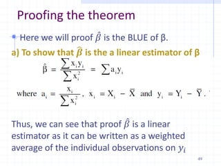
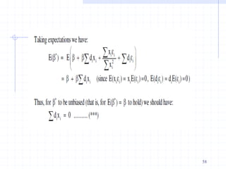
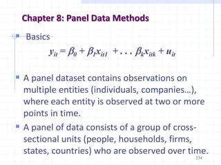
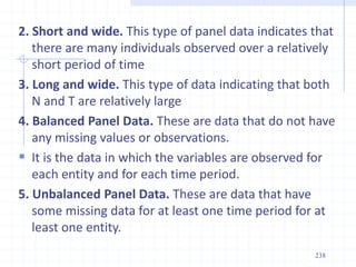
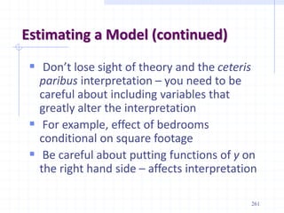
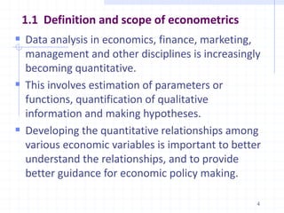
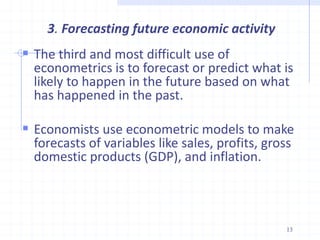
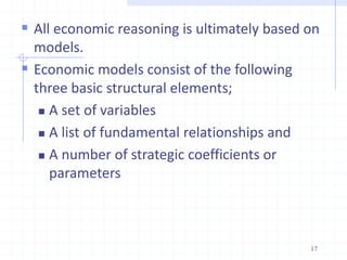
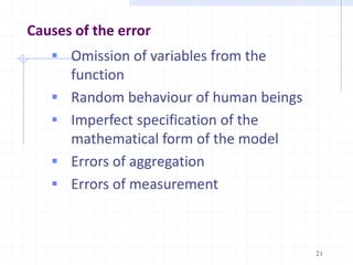
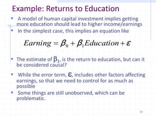
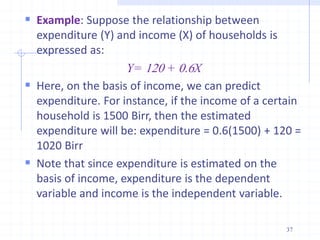
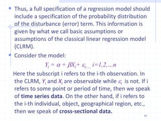
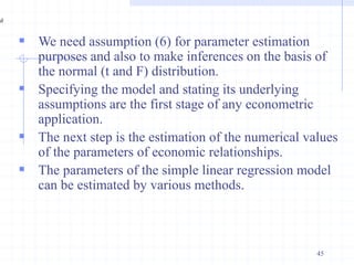
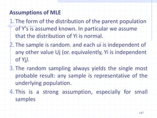
Proofing the Assumptions
 E(𝜀𝑖) = 0
 Var(𝜀𝑖) = E(𝜀𝑖 - E(𝜀𝑖))2 , but E(𝜀𝑖) = 0;
= E(𝜀𝑖 -0)2 = E(𝜀𝑖)2 = 𝜎2
 Ui~ N(0, 𝜎2) --- from equation 1 and 2
 Cov(𝑈𝑖, 𝑈𝑗) = E[(𝑈𝑖 –E(𝑈𝑖)][𝑈𝑗 – E(𝑈𝑗)]; since the E(𝑈𝑖) & E(𝑈𝑗)=0,
= E[(𝑈𝑖 – 0)(𝑈𝑗 – 0)]= E[(𝑈𝑖)(𝑈𝑗)] = E(𝑈𝑖) E(𝑈𝑗) = 0
 Cov(𝑋𝑖, 𝑈𝑖) = 0; E(𝑋𝑖–E(𝑋𝑖))(𝑈𝑖– E(𝑈𝑖), but the E(𝑈𝑖) = 0; then E(𝑋𝑖– E(𝑥𝑖))(𝑈𝑖)
= E(𝑋𝑖𝑈𝑖 – 𝑈𝑖E(𝑥𝑖) = 𝑋𝑖E(𝑈𝑖) – 𝑥𝑖E(𝑈𝑖) = 𝑋𝑖(o) – xi(0) = 0
83

 The only additional assumption here is that
there is no multicollinearity, meaning that
there is no linear dependence between the
regressor variables X2, X3, ….XK
 Under the above assumptions, ordinary least
squares (OLS) yields best linear unbiased
estimators (BLUE) of β2, β3, …. βK
84

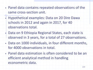
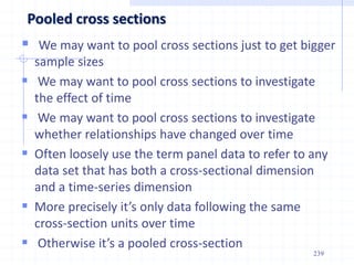
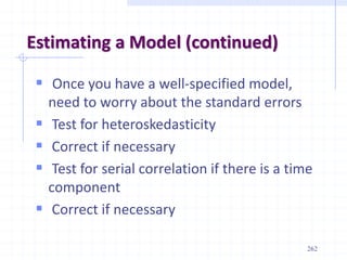
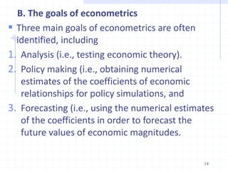
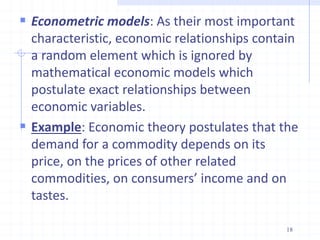
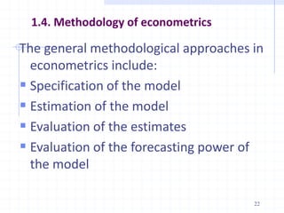
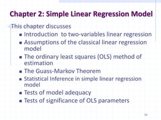
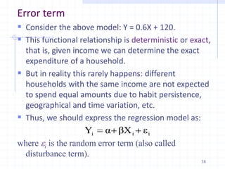
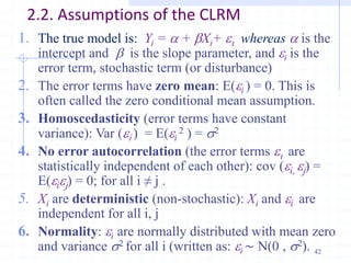
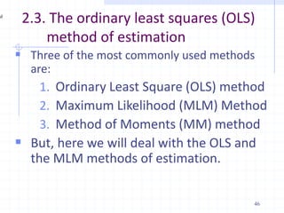
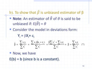
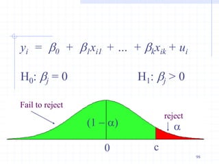
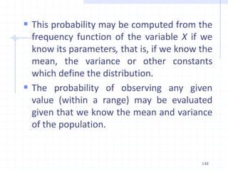
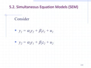
Consider the following equation:
Yi= b1 + b2X2i + b3X3i + . . . bkXki + i ,
For (k = 3), Yi= b1 + b2X2i + b3X3i + i
3.3. Estimation of parameters and SEs
  
  



 2
3
2
2
3
2
2
3
2
3
2
3
2
2
)
(
[
]
][
[
]
][
[
]
)
(
][
[
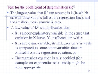
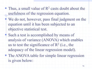
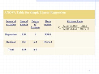
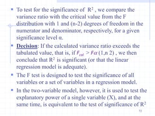
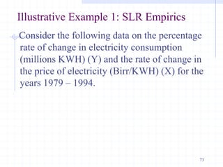
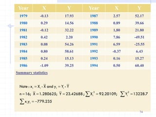
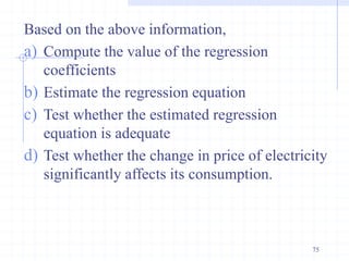
ˆ
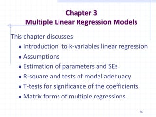
i
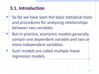
i
i
i
i
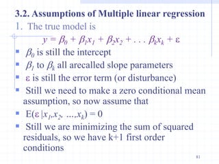
i
i
i
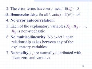
i
i
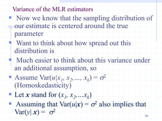
i
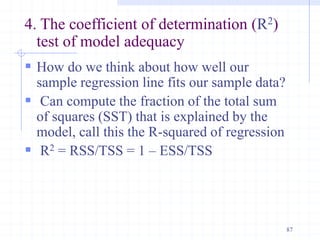
x
x
x
x
x
x
y
x
x
y
x
β
  
  



 2
3
2
2
3
2
2
3
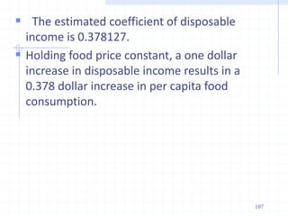
2
2
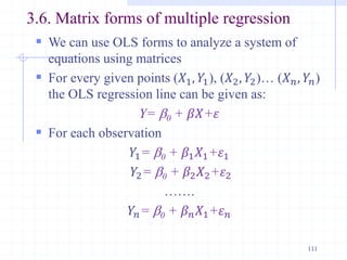
2
2
3
3
)
(
[
]
][
[
]
][
[
]
][
[
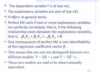
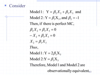
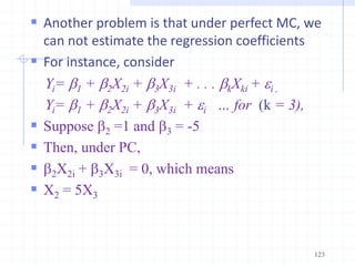
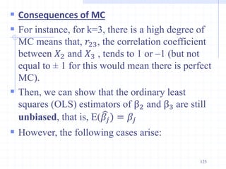
ˆ
i
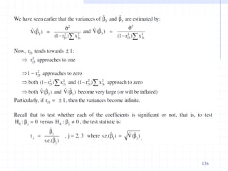
i
i
i
i
i
i
i
i
i
i
x
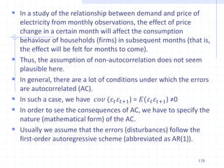
x
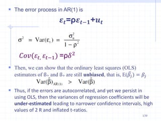
x
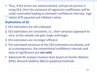
x
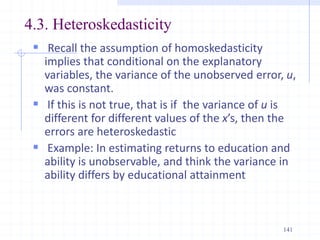
x
x
y
x
x
y
x
β
85

Variance of the MLR estimators
 Now we know that the sampling distribution of
our estimate is centered around the true
parameter
 Want to think about how spread out this
distribution is
 Much easier to think about this variance under
an additional assumption, so
 Assume Var(u|x1, x2,…, xk) = s2
(Homoskedasticity)
 Let x stand for (x1, x2,…xk)
 Assuming that Var(u|x) = s2 also implies that
Var(y| x) = s2
86

4. The coefficient of determination (R2)
test of model adequacy
 How do we think about how well our
sample regression line fits our sample data?
 Can compute the fraction of the total sum
of squares (SST) that is explained by the
model, call this the R-squared of regression
 R2 = RSS/TSS = 1 – ESS/TSS
87

More about R-squared
 R2 can never decrease when another
independent variable is added to a
regression, and usually will increase
 Because R2 will usually increase with the
number of independent variables, it is not a
good way to compare models
88

Too Many or Too Few Variables
 What happens if we include variables in
our specification that don’t belong?
 There is no effect on our parameter
estimate, and OLS remains unbiased
 What if we exclude a variable from our
specification that does belong?
 OLS will usually be biased
89

3.4. Inferences in multiple linear regression
 Consider, y = b0 + b1x1 + b2x2 + . . . bkxk + u
So far, we know that given the Gauss-Markov
assumptions, OLS is BLUE,
In order to do classical hypothesis testing, we
need to add another assumption (beyond the
Gauss-Markov assumptions)
Assume that u is independent of x1, x2,…, xk
and u is normally distributed with zero mean
and variance s2: u ~ Normal(0,s2)
90

 Under CLM, OLS estimators are BLUE,
with minimum variance unbiased estimator
 We can summarize the population
assumptions of CLM as follows
 y|x ~ Normal(b0 + b1x1 +…+ bkxk, s2)
 While for now we just assume normality,
clear that sometimes not the case
91

Normal sampling distributions
 
 
 
   
errors
the
of
n
combinatio
linear
a
is
it
because
normally
d
distribute
is
ˆ
0,1
Normal
~
ˆ
ˆ
that
so
,
ˆ
,
Normal
~
ˆ
s
t variable
independen
the
of
values
sample
the
on
l
conditiona
s,
assumption
CLM
Under the
j
b
b
b
b
b
b
b
j
j
j
j
j
j
sd
Var

92

The t - test
 
 
involved.
variables
of
number
k
size;
sample
n
,
1
:
freedom
of
degrees
the
Note
ˆ
by
estimate
to
have
we
because
normal)
(vs
on
distributi
a
is
this
Note
~
ˆ
ˆ
s
assumption
CLM
Under the
2
2
1
j







k
n
t
t
se k
n
j
j
s
s
b
b
b
93

 Knowing the sampling distribution for the
standardized estimator allows us to carry
out hypothesis tests
 Start with a null hypothesis
 For example, H0: bj=0
 If accept null, then accept that xj has no
effect on y, controlling for other x’s
 If we reject the null, we conclude that xj has
affects y, controlling for other x’s
94

 
0
ˆ
j
H
,
hypothesis
null
accept the
o
whether t
determine
to
rule
rejection
a
with
along
statistic
our
use
then
will
We
ˆ
ˆ
:
ˆ
for
statistic
the"
"
form
to
need
first
e
our test w
perform
To
t
se
t
t
j
j
j
b
b
b b

95

t -test: One-sided alternatives
 Besides our null, H0, we need an alternative
hypothesis, H1, and a significance level
 H1 may be one-sided, or two-sided
 H1: bj > 0 and H1: bj < 0 are one-sided
 H1: bj  0 is a two-sided alternative
 If we want to have only a 5% probability of
rejecting H0 if it is really true, then we say
our significance level is 5%
96

 Having picked a significance level, a, we
look up the (1 – a)th percentile in a t
distribution with n – k – 1 df and call this c,
the critical value
 We can reject the null hypothesis if the t
statistic is greater than the critical value
 If the t statistic is less than the critical value
then we fail to reject the null
97

yi = b0 + b1xi1 + … + bkxik + ui
H0: bj = 0 H1: bj > 0
c
0
a
1  a
Fail to reject
reject
98

One-sided vs two-sided
 Because the t distribution is symmetric,
testing H1: bj < 0 is straightforward.
 The critical value is just the negative of
before
 We can reject the null if the t statistic < –c,
and if the t statistic > than –c then we fail to
reject the null
 For a two-sided test, we set the critical
value based on a/2 and reject H1: bj  0 if
the absolute value of the t statistic > c
99

yi = b0 + b1Xi1 + … + bkXik + ui
H0: bj = 0 H1: bj > 0
c
0
a/2
1  a
-c
a/2
Two-sided alternatives
reject reject
fail to reject
100

Testing hypotheses
 A more general form of the t statistic
recognizes that we may want to test
something like H0: bj = aj
 In this case, the appropriate t statistic is
 
 
test
standard
for the
0
where
,
ˆ
ˆ



j
j
j
j
a
se
a
t
b
b
101

Computing p-values for t tests
 An alternative to the classical approach is
to ask, “what is the smallest significance
level at which the null would be rejected?”
 So, compute the t statistic, and then look up
what percentile it is in the appropriate t
distribution – this is the p-value
 p-value is the probability we would observe
the t statistic we did, if the null were true
102

Illustration 2: Multiple Linear Regression Empirics
Consider the following data of a country on per
capita food consumption (Y), price of food (X2
) and per capita income (X3 ) for the years
1927-1941. Retail price of food and per capita
disposable income are deflated by the
Consumer Price Index.
103

Year Y X2 X3 Year Y X2 X3
1927 88.9 91.7 57.7 1935 85.4 88.1 52.1
1928 88.9 92.0 59.3 1936 88.5 88.0 58.0
1929 89.1 93.1 62.0 1937 88.4 88.4 59.8
1930 88.7 90.9 56.3 1938 88.6 83.5 55.9
1931 88.0 82.3 52.7 1939 91.7 82.4 60.3
1932 85.9 76.3 44.4 1940 93.3 83.0 64.1
1933 86.0 78.3 43.8 1941 95.1 86.2 73.7
1934 87.1 84.3 47.8
Summary
statistics
56.52667
X
85.9
X
88.90667
Y
99.929
y
838.289
x
355.14
x
275.9
x
x
257.397
y
x
27.63
y
x
15;
n
Y
-
Y
y
and
X
-
X
x
,
X
-
X
x
:
Note
3
2
2
2
3
2
2
3
2
3
2
i
i
3
3i
i
3
2
i
2
i
2



















104

Required: Based on the above information,
a) Compute the value of OLS estimators of the
regression coefficients, 𝛽1, 𝛽2and 𝛽3
c) Test whether the estimated regression equation
is adequate
d) Test whether the price of food and per capita
income significantly affects per capita food
consumption
e) Suppose that, in 1945, the price of food and per
capita income are Birr 90 and Birr 75,
respectively, compute the per capita food
consumption in 1945.
105

Generally we have the following:
 Food price significantly and negatively affects
per capita food consumption, while disposable
income significantly and positively affects per
capita food consumption.
 The estimated coefficient of food price is -
0.21596.
 Holding disposable income constant, a one
dollar increase in food price results in a 0.216
dollar decrease in per capita food
consumption.
106

 The estimated coefficient of disposable
income is 0.378127.
 Holding food price constant, a one dollar
increase in disposable income results in a
0.378 dollar increase in per capita food
consumption.
107

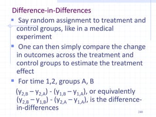
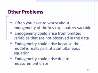
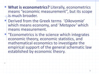
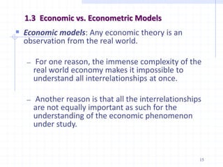
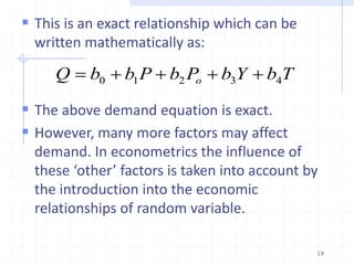
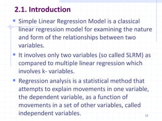
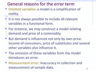
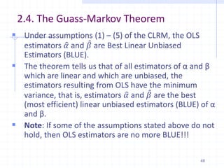
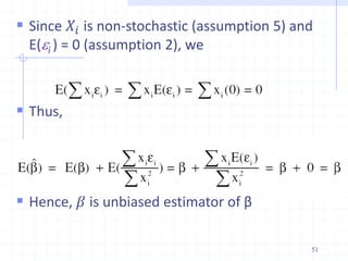
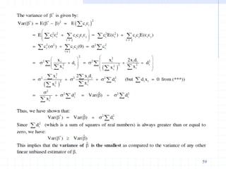
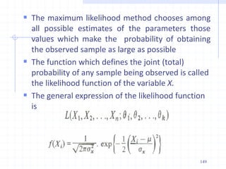
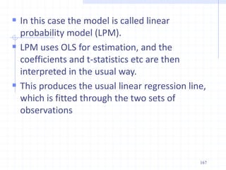
Computing p-values and t tests with
statistical packages
 Most computer packages will compute the
p-value for you, assuming a two-sided test
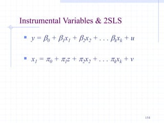
 If you really want a one-sided alternative,
just divide the two-sided p-value by 2
 Stata provides the t statistic, p-value, and
95% confidence interval for H0: bj = 0 for
you, in columns labeled “t”, “P > |t|” and
“[95% Conf. Interval]”, respectively
108

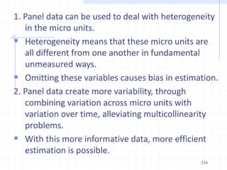
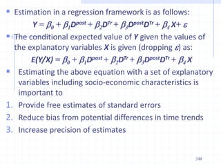
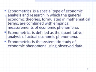
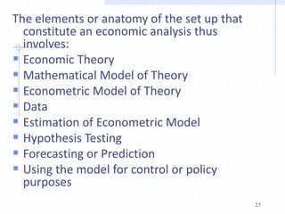
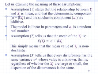
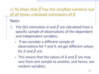
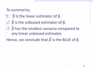
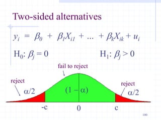
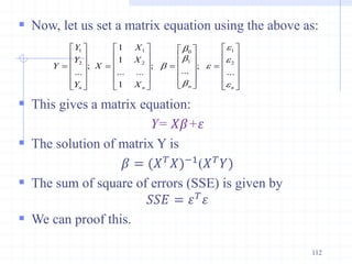
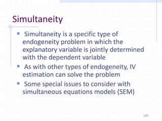
109
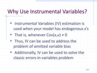
 Given multiple regression stata output for income as dependent
variable and temperature, altitude, cities, wage, education,
ownership, and location as explanatory variables and _cons is a
constant term. Based on this, answer the questions that follow.
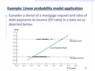
 The following table is generated using the command..
regress income temperature altitude cities wage education
ownership location
_cons .388519 .2026306 1.92 0.058 -.0126417 .7896797
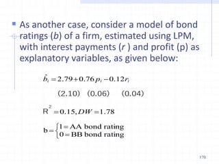
location -.0334028 .009427 -3.54 0.001 -.0520661 -.0147395
ownership .1559908 .0977688 1.60 0.113 -.0375684 .34955
education .0430756 .0125391 3.44 0.001 .0182511 .0679001
wage .1425848 .0795389 1.79 0.076 -.0148835 .300053
cities -.4307053 .0685673 -6.28 0.000 -.5664523 -.2949584
altitude .002892 .0815342 0.04 0.972 -.1585266 .1643105
temperature .0498639 .0681623 0.73 0.466 -.0850814 .1848092
income Coef. Std. Err. t P>|t| [95% Conf. Interval]

Questions
 Which of the explanatory variables do
significantly affect the income level at 1%
significance level?
 Which of the explanatory variables do not
significantly affect the income level at 1%
significance level?
 Which of the explanatory variables significantly
negatively affect the income level at 1%
significance level?
 Identify a variable which is not significant at 5%,
but remains significant at 10% level.
 Identify variables which are insignificant.
110

3.6. Matrix forms of multiple regression
 We can use OLS forms to analyze a system of
equations using matrices
 For every given points (𝑋1, 𝑌1), (𝑋2, 𝑌2)… (𝑋𝑛, 𝑌𝑛)
the OLS regression line can be given as:
Y= b0 + 𝛽𝑋+𝜀
 For each observation
𝑌1= b0 + 𝛽1𝑋1+𝜀1
𝑌2= b0 + 𝛽2𝑋2+𝜀2
…….
𝑌𝑛= b0 + 𝛽𝑛𝑋1+𝜀𝑛
111

 Now, let us set a matrix equation using the above as:
 This gives a matrix equation:
Y= 𝑋𝛽+𝜀
 The solution of matrix Y is
𝛽 = (𝑋𝑇𝑋)−1(𝑋𝑇𝑌)
 The sum of square of errors (SSE) is given by
𝑆𝑆𝐸 = 𝜀𝑇𝜀
 We can proof this.
112




















































n
n
n
n X
X
X
X
Y
Y
Y
Y




b
b
b
b
...
;
...
;
1
...
...
1
1
;
...
2
1
1
0
2
1
2
1

 In using OLS, we are minimizing the ESS
 𝐸𝑆𝑆 = 𝜀1
2
+𝜀2
2
+…+𝜀𝑛
2
 In matrix form, this means
 𝐸𝑆𝑆 = 𝜀1 𝜀2 … 𝜀𝑛
𝜀1
𝜀2
…
𝜀𝑛
 𝐸𝑆𝑆 = 𝜀𝑇𝜀; since 𝜀 = 𝑦 − 𝑋𝛽
 𝐸𝑆𝑆 = 𝑦 − 𝑋𝛽
𝑇
𝑦 − 𝑋𝛽
113

 Using the apostrophe for the transpose, we have
𝐸𝑆𝑆 = 𝑦 − 𝑋𝛽
′
𝑦 − 𝑋𝛽
𝐸𝑆𝑆 = (𝑦′−𝛽′𝑋′) 𝑦 − 𝑋𝛽
𝐸𝑆𝑆 = 𝑦′
𝑦 − 𝑦′
𝑋𝛽 − 𝛽′
𝑋′
y+𝛽′
𝑋′
𝑋𝛽
𝜕𝐸𝑆𝑆
𝜕𝛽
=0 − 𝑋′y − 𝑋′y+2𝑋′𝑋𝛽 = 0
−2𝑋′y+2𝑋′𝑋𝛽 = 0
𝑋′𝑋𝛽 = 𝑋′y
(𝑋′
𝑋)−1
𝑋′
𝑋𝛽 = (𝑋′
𝑋)−1
𝑋′
y
𝛽 = (𝑋′
𝑋)−1
𝑋′
y
114

Illustration: Determining OLS regression line using matrix
Consider the following data for the price in (ETB) and
demand in units for a product.
Required: Based on the above information,
a) Compute the value of OLS estimators of the regression
coefficients,𝛽2and 𝛽3 using the matrix approach.
c) Compute the sum of the squares of the errors (SSE).
d) Suppose that the price of the product is ETB 54,
compute the amount of quantity demanded. 115
Price in ETB and demand in units
Price (x) 49 69 89 99 109
Demand (y) 124 95 71 45 18

 Remember that:
116

b




b
b
b
b




























































































X
Y
X
Y
X
X
X
X
Y
Y
Y
Y
n
n
n
n
109
99
89
69
49
1
1
1
1
1
18
45
71
95
124
...
...
1
...
...
1
1
...
2
1
1
0
2
1
2
1

 Now using Y= 𝑋𝛽+𝜀, we need to find X using
𝛽 = (𝑋𝑇𝑋)−1(𝑋𝑇𝑌)
117


























































































a
c
b
d
bc
ad
d
c
b
a
A
X
X
X
X
X
Y
1
A
then
,
if
Recall,
;
5
415
415
36765
11600
1
)
(
36765
415
415
5
109
1
99
1
89
1
69
1
49
1
109
99
89
69
49
1
1
1
1
1
;
109
99
89
69
49
1
1
1
1
1
;
18
45
71
95
124
1
-
1
'
'
1
0
b
b
b

 Next we need to get, 𝑋𝑇𝑌
118
values.
residual
the
compute,
can
we
n,
observatio
each
For
:
Note
X̂
1.7
-
211
Ŷ
-1.7;
and
211
Hence,
7
.
1
211
25367
353
5
415
415
36765
11600
1
)
(
25367
353
18
45
71
95
124
109
99
89
69
49
1
1
1
1
1
1
0
'
1
'
1
0
'

































































b
b
b
b
b Y
X
X
X
Y
X

 Now, we can add, 𝜀𝑖 = 𝑦𝑖 − 𝑦𝑖, to compute the individual residual values
and the total SSE (See the last row in Table below).
Note:
 The error sum of squares (ESS) or sum of squares of errors (SSE) is Br.
208.
 At the price of ETB 54, 𝑌 = 211 − 1.7 54 = 211 − 91.8 = 119.2
 Therefore, according to the model, if the price is ETB 54, we expect that
the quantity demanded is about 119 units.
119
Price (x) 49 69 89 99 109
Demand (y) 124 95 71 45 18
DD estimate (𝑦) 127.7 93.7 59.7 42.7 25.7
𝜀𝑖 = 𝑦𝑖 − 𝑦𝑖 -3.7 1.3 11.3 2.3 -7.7
  65
.
207
7
.
7
3
.
2
3
.
11
3
.
1
7
.
3
7
.
7
3
.
2
3
.
11
3
.
1
7
.
3
;
7
.
7
3
.
2
3
.
11
3
.
1
7
.
3








































 SSE


Chapter 4: Estimation problems under
violations of the assumptions of OLS
4.1. Multicollinearity
 In the construction of an econometric model, it
may happen that two or more variables giving rise
to the same piece of information are included,
 That is, we may have redundant information or
unnecessarily included related variables
 This is what we call a multicollinearity (MC)
problem.
120

 The dependent variable Y is of size nx1.
 The explanatory variables are also of size nX1.
 Y=Xβ+𝜀, in general terms
 Perfect MC exits if two or more explanatory variables
are perfectly correlated, that is, if the following
relationship exists between the explanatory variables,
that is,
 One consequence of perfect MC is non-identifiability
of the regression coefficient vector β .
 This means that one can not distinguish between two
different models: Y = Xβ + ε and Y = X𝛽 +ε .
 These two models are said to be observationally
equivalent.
121
0
...
3
3
2
2 

 n
n X
X
X b
b
b

 Consider
122
.
equivalent
nally
observatio
are
2
Model
and
1
Model
Therefore,
X
Y
:
2
Model
X
2
Y
:
1
Model
,
0
0
MC,
perfect
is
there
if
Then,
-1
and
,
X
Y
:
2
Model
and
Y
:
1
Model
3
3
3
3
3
3
2
3
3
2
3
3
2
2
2
3
3
3
3
2
2
b
b
b
b
b
b
b
b
b
b












Thus
X
X
X
X
X
X
X
X

 Another problem is that under perfect MC, we
can not estimate the regression coefficients
 For instance, consider
Yi= b1 + b2X2i + b3X3i + . . . bkXki + i ,
Yi= b1 + b2X2i + b3X3i + i … for (k = 3),
 Suppose b2 =1 and b3 = -5
 Then, under PC,
 b2X2i + b3X3i = 0, which means
 X2 = 5X3
123

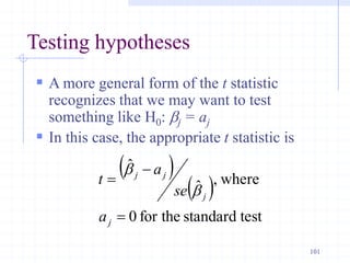
 Consider parametric estimation under MLR
 Thus, b2 is indeterminate. It can also be shown that b3 is also
indeterminate. Therefore, in the presence of perfect MC, the
regression coefficients can not be estimated.
     
    
     
     0
0
25
25
5
5
ˆ
)
5
(
)
5
(
5
5
ˆ
)
(
[
]
][
[
]
][
[
]
)
(
[
]
[
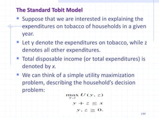
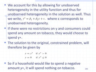
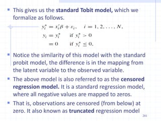
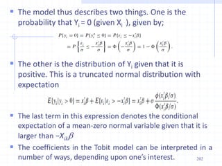
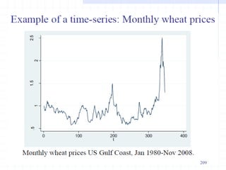
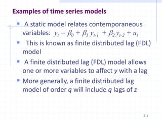
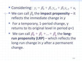
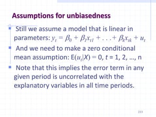
ˆ
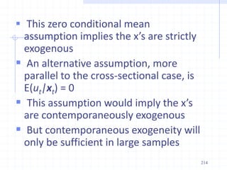
2
2
3
2
3
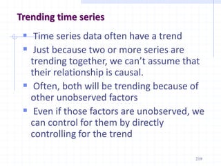
2
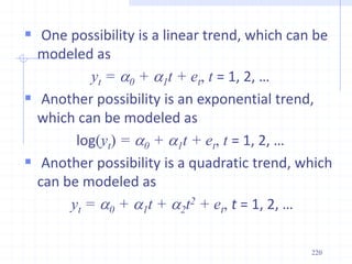
3
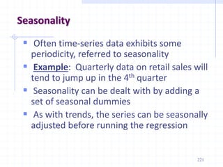
2
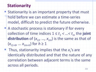
3
3
2
3
3
2
2
3
3
2
3
2
3
3
3
3
2
3
3
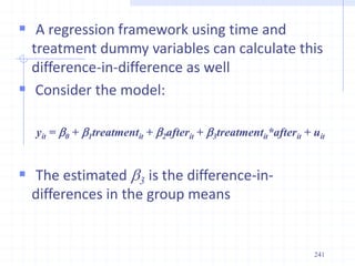
2
2
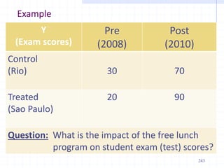
3
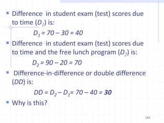
2
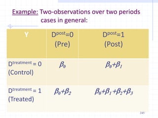
2
3
2
2
3
2
3
2
3
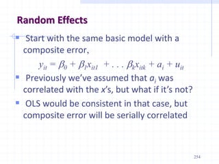
2
2
























  
  

x
x
x
x
y
x
x
y
x
x
x
x
x
x
x
y
x
x
y
x
x
x
x
x
x
x
y
x
x
y
x
i
i
i
i
i
i
i
i
i
i
i
i
i
i
i
i
i
i
i
b
b
b
124

 Consequences of MC
 For instance, for k=3, there is a high degree of
MC means that, 𝑟23, the correlation coefficient
between 𝑋2 and 𝑋3 , tends to 1 or –1 (but not
equal to ± 1 for this would mean there is perfect
MC).
 Then, we can show that the ordinary least
squares (OLS) estimators of β2 and β3 are still
unbiased, that is, E(𝛽𝑗) = 𝛽𝑗
 However, the following cases arise:
125

 Thus, under a high degree of MC, the
standard errors will be inflated and the test
statistic will be a very small number.
 This often leads to incorrectly accepting
(not rejecting) the null hypothesis when in
fact the parameter is significantly different
from zero!
 Mostly, two extreme cases rarely exist in
practice, and of particular interest are cases
in between: moderate to high degree of MC
127

 Such kind of MC is so common in
macroeconomic time series data (such as GNP,
money supply, income, etc) since economic
variables tend to move together over time.
Consequences of MC
 Under a high degree of MC, the standard errors
will be inflated and the test statistic will be a
very small number.
 This often leads to incorrectly accepting (not
rejecting) the null hypothesis when in fact the
parameter is significantly different from zero!
128

Major implications of a high degree of MC
1. OLS coefficient estimates are still unbiased.
2. OLS coefficient estimates will have large variances (or
the variances will be inflated).
3. There is a high probability of accepting the null
hypothesis of zero coefficient (using the t-test) when
in fact the coefficient is significantly different from
zero.
4. The regression model may do well, that is, R-squared
may be quite high.
5. The OLS estimates and their standard errors may be
quite sensitive to small changes in the data.
129

Methods of detection of MC
 Multicollinearity almost always exists in most
applications.
 So the question is not whether it is present or
not; it is a question of degree!
 MC is not a statistical problem; it is a data
(sample) problem.
 Therefore, we do not “test for MC’’; but
measure its degree in any particular sample
(using some rules of thumb).
130

 The speed with which variances and co-
variances increase can be seen with the
variance-inflating factor (VIF)
 VIF shows how the variance of an estimator
is inflated by the presence of
multicollinearity
 There is multicollinearity if VIF > 10, but
multicollinearity is not a problem if VIF < 10.
131

Some of the other methods of detecting MC are:
1. High R2 but few (or no) significant t-ratios.
2. High pair-wise correlations among regressor.
Note that this is a sufficient but not a necessary
condition; that is, small pair-wise correlation for
all pairs of regressors does not guarantee the
absence of MC.
132

Remedial measures
To circumvent the problem of MC, some of the
possibilities are:
1. Dropping a variable. This may result in an incorrect
specification of the model (called specification bias).
For instance, GDP and consumption do have an impact
on imports, so dropping one or the other, introduces
specification bias.
133

2. Transformation of variables
 By transforming the variable, it could be
possible to reduce the effect of
multicollinearity.
3. Increasing the sample size
 By increasing the sample, high covariances among
estimated parameters resulting from multicollinearity
in an equation can be reduced, because these
covariances are inversely proportional to sample size.
134

4.2. Autocorrelation
 Autocorrelation exists when two or more error
terms are serially correlated.
 Non-autocorrelation or absence of serial
correlation assumption tells us that the error
term at time t is not correlated with the error
term at any other point of time.
 This means that when observations are made
over time, the effect of the disturbance occurring
at one period does not carry-over into another
period.
135

 In case of cross-sectional data such as those on
income and expenditure of different
households, the assumption of non-
autocorrelation is plausible since the
expenditure behaviour of one household does
not affect the expenditure behaviour of any
other household in general.
 The assumption of non-autocorrelation is more
frequently violated in case of relations
estimated from time series data.
136

 For instance, in a study of the relationship
between output and inputs of a firm or industry
from monthly observations, non-
autocorrelation of the disturbance implies that
the effect of machine breakdown is strictly
temporary in the sense that only the current
month’s output is affected.
 But in practice, the effect of a machine
breakdown in one month may affect current
month’s output as well as the output of
subsequent months.
137

 In a study of the relationship between demand and price of
electricity from monthly observations, the effect of price
change in a certain month will affect the consumption
behaviour of households (firms) in subsequent months (that is,
the effect will be felt for months to come).
 Thus, the assumption of non-autocorrelation does not seem
plausible here.
 In general, there are a lot of conditions under which the errors
are autocorrelated (AC).
 In such a case, we have 𝑐𝑜𝑣 (𝜀𝑡𝜀𝑡+1) = 𝐸(𝜀𝑡𝜀𝑡+1) ≠0
 In order to see the consequences of AC, we have to specify the
nature (mathematical form) of the AC.
 Usually we assume that the errors (disturbances) follow the
first-order autoregressive scheme (abbreviated as AR(1)).
138

 The error process in AR(1) is
𝜺𝒕=ρ𝜺𝒕−𝟏+𝒖𝒕
 Then, we can show that the ordinary least squares (OLS)
estimators of β2 and β3 are still unbiased, that is, E(𝛽𝑗) = 𝛽𝑗
 Thus, if the errors are autocorrelated, and yet we persist in
using OLS, then the variances of regression coefficients will be
under-estimated leading to narrower confidence intervals, high
values of 2 R and inflated t-ratios.
139
𝐶𝑜𝑣(𝜀𝑡, 𝜀𝑡−1) =ρ𝛿2

 Thus, if the errors are autocorrelated, and yet we persist in
using OLS, then the variances of regression coefficients will be
under-estimated leading to narrower confidence intervals, high
values of R-squared and inflated t-ratios.
Implications of AC
1. OLS estimators are still unbiased.
2. OLS estimators are consistent, i.e., their variances approach to
zero, as the sample size gets larger and larger.
3. OLS estimators are no longer efficient.
4. The estimated variances of the OLS estimators are biased, and
as a consequence, the conventional confidence intervals and
tests of significance are not valid.
 Advanced AC analysis involves tests based on Durbin-Watson
(DW), Breusch-Godfrey (BG) or graphical methods.
140

4.3. Heteroskedasticity
 Recall the assumption of homoskedasticity
implies that conditional on the explanatory
variables, the variance of the unobserved error, u,
was constant.
 If this is not true, that is if the variance of u is
different for different values of the x’s, then the
errors are heteroskedastic
 Example: In estimating returns to education and
ability is unobservable, and think the variance in
ability differs by educational attainment
141

.
x
x1 x2
f(y|x)
Example of Heteroskedasticity
x3
.
. E(y|x) = b0 + b1x
142

 Thus under heteroschedasticity,
𝑣𝑎𝑟(ε𝑖)=E(𝜀2
) = 𝑘𝛿2
instead of
𝑣𝑎𝑟(ε𝑖)=E(𝜀2
) = 𝛿2
𝑉𝑎𝑟(𝛽𝐻𝐸𝑇) =
 If k=1, 𝑉𝑎𝑟(𝛽𝐻𝐸𝑇)= 𝑉𝑎𝑟(𝛽𝑖), but
143

 Thus, under heteroscedasticity, the OLS
estimators of the regression coefficients are not
BLUE and efficient.
 Generally, under error heteroscedasticity we have
the following:
1. The OLS estimators of the regression coefficients
are still unbiased and consistent.
2. The estimated variances of the OLS estimators are
biased and the conventionally calculated confidence
intervals and test of significance are invalid.
144

Consequences Heteroskedasticity
 OLS is still unbiased and consistent, even if
we do not assume homoskedasticity
 The standard errors of the estimates are
biased if we have heteroskedasticity
 If the standard errors are biased, we can not
use the usual t statistics or F statistics
statistics for drawing inferences
 The remedy is to use robust SEs and there
are also tests.
145

Chapter 5: Other Estimation Techniques
5.1. Maximum likelihood method
 The maximum likelihood method is another
method for obtaining estimates of the parameters
of a population from a random sample
 Assume we take a sample of n values of X drawn
randomly from the population of (all possible
values of) X.
 Each observation of the sample has a certain
probability of occurring in any random drawing
146

Assumptions of MLE
1.The form of the distribution of the parent population
of Y's is assumed known. In particular we assume
that the distribution of Yi is normal.
2.The sample is random. and each ui is independent of
any other value Uj (or. equivalently, Yi is independent
of Yj).
3.The random sampling always yields the single most
probable result: any sample is representative of the
underlying population.
4.This is a strong assumption, especially for small
samples
147

 This probability may be computed from the
frequency function of the variable X if we
know its parameters, that is, if we know the
mean, the variance or other constants
which define the distribution.
 The probability of observing any given
value (within a range) may be evaluated
given that we know the mean and variance
of the population.
148

 The maximum likelihood method chooses among
all possible estimates of the parameters those
values which make the probability of obtaining
the observed sample as large as possible
 The function which defines the joint (total)
probability of any sample being observed is called
the likelihood function of the variable X.
 The general expression of the likelihood function
is
149

The total probability of obtaining all the values in the sample is the
product of the individual probabilities given that each observation
is independent of the others
150

 Since log L is a monotonic function of L, the values of the
parameters that maximise log L will also maximise L.
 Thus we maximise the logarithmic expression of the likelihood
function by setting its partial derivatives with respect to
equal to zero.
151

5.2. Simultaneous Equation Models (SEM)
Consider
 y1 = a1y2 + b1z1 + u1
 y2 = a2y1 + b2z2 + u2
152

Simultaneity
 Simultaneity is a specific type of
endogeneity problem in which the
explanatory variable is jointly determined
with the dependent variable
 As with other types of endogeneity, IV
estimation can solve the problem
 Some special issues to consider with
simultaneous equations models (SEM)
153

Instrumental Variables & 2SLS
 y = b0 + b1x1 + b2x2 + . . . bkxk + u
 x1 = p0 + p1z + p2x2 + . . . pkxk + v
154

Why Use Instrumental Variables?
 Instrumental Variables (IV) estimation is
used when your model has endogenous x’s
 That is, whenever Cov(x,u) ≠ 0
 Thus, IV can be used to address the
problem of omitted variable bias
 Additionally, IV can be used to solve the
classic errors-in-variables problem
155

What Is an Instrumental Variable?
 In order for a variable, z, to serve as a valid
instrument for x, the following must be true
 The instrument must be exogenous
 That is, Cov(z,u) = 0
 The instrument must be correlated with
the endogenous variable x
 That is, Cov(z,x) ≠ 0
156

Two Stage Least Squares (2SLS)
 It’s possible to have multiple instruments
 Consider our original structural model, and
let y2 = p0 + p1z1 + p2z2 + p3z3 + v2
 Here we’re assuming that both z2 and z3
are valid instruments – they do not appear
in the structural model and are
uncorrelated with the structural error term,
u1
157

Chapter 6
Limited Dependent Variable Models
 In regression analysis, the dependent variable, Y,
is frequently not only quantitative continuous
variable (e.g. income, output, prices, costs,
height, temperature).
 But it can also be qualitative (E.g., dummy,
ordinal and truncated).
 For instance, consider sex, race, color, religion,
nationality, geographical region, political
upheavals, and party affiliation as variables.
158

 There are many examples of this type of
models.
 For instance, if we want to examine
determinants of using mobile banking
 This means that for all observations
(customers) i of a bank, we give the value 0 for
those who do not use mobile banking, and 1
for those who uses mobile banking services .




users
non-
banking
mobile
0,
users
banking
mobile
for
1,
Yi
159

 Dummy variables can also be used in
regression analysis just as quantitative
variables, being both dependent or
independent variable.
 For instance, we can denote the dummy
explanatory variables by the symbol D rather
than by the usual symbol X to emphasize that
we are dealing with a qualitative variable.
 As a matter of fact, a regression model may
contain only dummy explanatory variables.
160

 Consider the following example of such a
model:
where Y = annual expenditure on food ($); Di =
1 if female; Di = 0 if male
161

 Therefore the values obtained, b1 and b2 ,
enable us to estimate the probabilities
 In using dummy variable models, we
consider the case where the dependent
variable can take the value of 0 or 1.
 They are often termed dichotomous
variables
 These types of model tend to be associated
with the cross-sectional econometrics rather
than time series.
162

6.2. Data
 When examining the dummy dependent
variables, we need to ensure there are
sufficient numbers of 0s and 1s.
 For instance, to assess mobile banking users,
we need a sample of both: users who have
mobile banking services and non-users who
have no mobile banking services.
 It is easier to find data for both category of
customers, users and non-users.
 Three basic models: linear probability, Logit
and Probit models are mostly used to analyze
such data.
164

6.3. Linear Probability Model (LPM)
 It is among discrete choice models or
dichotomous choice models.
 In this case the dependent variable takes only
two values: 0 and 1.
 There are several methods to analyze
regression models where the dependent
variable is 0 or 1.
 The simplest method is to use the least
squares method.
165

Example: Linear probability model application
Consider a denial of a mortgage request and ratio of
debt payments to income (P/I ratio) in a data set as
depicted below:
166

 In this case the model is called linear
probability model (LPM).
 LPM uses OLS for estimation, and the
coefficients and t-statistics etc are then
interpreted in the usual way.
 This produces the usual linear regression line,
which is fitted through the two sets of
observations
167

Features of the LPM
 The dependent variable has two values, the
value 1 has a probability of p and the value 0
has a probability of (1-p)
 This is known as the Bernoulli probability
distribution.
 In this case the expected value of a random
variable following a Bernoulli distribution is
the probability that the variable equals 1
 Since the probability of p must lie between 0
and 1, then the expected value of the
dependent variable must also lie between 0
and 1.
168

 The error term is not normally distributed,
it also follows the Bernoulli distribution
 The variance of the error term is
heteroskedastistic.
 The variance for the Bernoulli distribution is
p(1-p), where p is the probability of a
success.
 The value of the R-squared statistic is
limited, given the distribution of the LPMs.
169

 As another case, consider a model of bond
ratings (b) of a firm, estimated using LPM,
with interest payments (r ) and profit (p) as
explanatory variables, as given below:











rating
bond
BB
0
rating
bond
AA
1
b
.
,
.
.
.
.
ˆ
78
1
15
0
12
0
76
0
79
2
DW
r
p
b i
i
i
2
R
(0.04)
(0.06)
(2.10)
170

 The coefficients are interpreted as in the
usual OLS models, i.e. a 1% rise in profits,
gives a 0.76% increase in the probability of
a bond getting the AA rating.
 The R-squared statistic is low, but this is
probably due to the LPM approach, so we
would usually ignore it.
 The t-statistics are interpreted in the usual
way.
171

Problems with LPM
 Possibly the most problematic aspect of the
LPM is the non-fulfillment of the requirement
that the estimated value of the dependent
variable y lies between 0 and 1.
 One way around the problem is to assume
that all values below 0 and above 1 are
actually 0 or 1 respectively
 Another problem with the LPM is that it is a
linear model and assumes that the probability
of the dependent variable equalling 1 is
linearly related to the explanatory variable.
172

 For example, if we have a model where the
dependent variable takes the value of 1 if a
mortgage is granted to a bank customer and 0
otherwise, regressed on the customer’s income.
 The probability of being granted a mortgage
will rise steadily at low income levels, but
change hardly at all at high income levels.
 An alternative and much better remedy to the
problem is to use an alternative technique such
as the Logit or Probit models.
173

6.4. Logit Model
 The main way around the problems mentioned
earlier is to use a different distribution to the
Bernoulli distribution, where the relationship
between x and p is non-linear and the p is
always between 0 and 1.
 This requires the use of ‘S’ shaped distribution
curves, which resemble the cumulative
distribution function (CDF) of a random
variable.
 The CDFs used to represent a discrete variable
are the logistic (Logit model) and normal
(Probit model).
174

The problem with the linear probability model is
that it models the probability of Y = 1 as being
linear:
Instead, we aim to construct:
 0 ≤ Pr(Y = 1|X) ≤ 1 for all X.
 Pr(Y = 1|X) to be increasing in X (for > 0).
 This requires a nonlinear functional form for
the probability.
 Both Logit and Probit models which are “S-
curve” can be used. 175

The probit and logit models satisfy these conditions:
 0 ≤ Pr(Y = 1|X) ≤ 1 for all X.
 Pr(Y = 1|X) to be increasing in X (for > 0).
176

 For instance, assume that we have the
following basic model, expressing the
probability that y=1 as a cumulative
logistic distribution function:
i
i
i
i
i
i
x
x
y
E
p
u
X
Y
1
0
1
0
1 β
β
β
β







)
/
(
177

 The cumulative logistic distributive function
can then be written as:
i
i
z
i
x
β
β
z
e
p i
1
0
1
1



 
:
Where
178

 There is a problem with non-linearity
in the previous expression, but this can
be solved by creating the odds ratio:
i
i
i
i
i
z
z
z
i
i
z
i
x
β
β
z
)
p
p
(
L
e
e
e
p
p
e
p
i
i
i
i
1
0
1
1
1
1
1
1
1














ln
179

 In the previous slide L is the log of the odds
ratio and is linear in the parameters.
 The odds ratio can be interpreted as the
probability of something happening to the
probability it won’t happen.
 For the mortgage case, the odds ratio of
getting a mortgage is the probability of
getting a mortgage to the probability of not
getting mortgage.
 If p is 0.8, , the odds are 4 to 1, which means
the probability of getting mortgage to not
getting it is 4:1.
180

Features of the Logit model
 Although L is linear in the parameters, the
probabilities are non-linear.
 The Logit model can be used in multiple regression
tests.
 If L is positive, as the value of the explanatory
variables increase, the odds that the dependent
variable equals 1 increases.
 The slope coefficient measures the change in the
log-odds ratio for a unit change in the explanatory
variable.
 Logit and Probit models are usually estimated
using Maximum Likelihood techniques.
181

 The R-squared statistic is not suitable for
measuring the goodness-of-fit in discrete
dependent variable models, instead we
compute the count R-squared statistic.
 If we assume any probability greater than
0.5 counts as a 1 and any probability less
than 0.5 counts as a 0, then we count the
number of correct predictions.
 This is defined as count R-squared as
follows:
ns
observatio
of
number
Total
s
prediction
correct
of
number
R
Count
2

182

 The Logit model can be interpreted in a
similar way to the LPM
 For instance, consider the previous model
where the dependent variable is granting of
a mortgage (1) or not (0).
 The explanatory variable is income of
customers.
 The coefficient on y suggests that a 1%
increase in income (y) produces a 0.32%
rise in the log of the odds of getting a
mortgage. 183

 This is difficult to interpret, so the
coefficient is often ignored, the z-statistic
(same as t-statistic) and sign on the
coefficient is however used for the
interpretation of the results.
 We can transform the natural log for
interpretation.
 We could also include a specific value for
the income of a customer and then find
the probability of getting a mortgage.
184

Logit Result
 If we have a customer with 0.5 units of
income, we can estimate a value for the Logit
of 0.56+0.32*0.5 = 0.72.
 We can use this estimated Logit value to find
the estimated probability of getting a
mortgage.
 By including it in the formula given earlier for
the Logit Model we get:
67
.
0
49
.
1
1
)
1
(
1
)
72
.
0
(



 
e
pi
185

 Given that this estimated probability is
bigger than 0.5, we assume it is nearer 1,
therefore we predict this customer would
be given a mortgage.
 With the Logit model we tend to report the
sign of the variable and its z-statistic which
is the same as the t-statistic in large
samples.
186

6.5. The Probit Model
 An alternative approach, called by
Goldberger (1964) is the Probit model
 The Probit model assumes that there is an
underlying response variable defined by
the following regression relationship.
 is unobserved, it is referred to as a
latent variable.
187

 The latent variable generates the observed
y’s.
 Those who have larger values of the latent
variable are observed as y = 1 and those
who have smaller values are observed as y
= 0
 We observe the dummy variable y defined
as;
188

 An alternative CDF to that used in the Logit
Model is the normal CDF, when this is used
we refer to it as the Probit Model.
 In many respects this is very similar to the
Logit model.
 The Probit model has also been interpreted as
a ‘latent variable’ model.
 This has implications for how we explain the
dependent variable. i.e. we tend to interpret
it as a desire or ability to achieve something.
189

LPM, Logit and Probit models compared
 The coefficient estimates from all three models
are related, because with Bernoulli, logistic and
normal distribution function differences .
 If you multiply the coefficients from a Logit
model by 0.625, they are approximately the
same as the Probit model.
 If the coefficients from the LPM are multiplied
by 2.5 (also 1.25 needs to be subtracted from
the constant term) they are approximately the
same as those produced by a Probit model.
190

 In general, dummy variables can also be
used as the dependent variable
 The LPM is the basic form of this model,
but has a number of important faults.
 The Logit model is an important
development on the LPM, overcoming
many of these problems.
 The Probit is similar to the Logit model but
assumes a different CDF, i.e., normal
distribution function.
191

Models for ordinal outcomes
 The categories of an ordinal variable can be
ranked from low to high, but the distances
between the categories are unknown.
 Ordinal outcomes are common in social
sciences.
 For example, in a survey research, opinions are
often ranked as strongly agree, agree, neutral,
disagree, and strongly disagree.
 Performance can be ranked as very high, high,
medium, low and very low.
192

Models for ordinal outcomes...
 Such data appear without any assumption that
the distance from strongly agreeing and
agreeing is the same as the distance from
agree to disagree.
 Educational attainments can be ordered as
elementary education, high school diploma,
college diploma, and graduate or professional
degree.
 An ordinal dependent variable violates the
assumptions of the logistic regression model,
which can lead to incorrect conclusions.
193

 Accordingly, with ordinal outcomes, it is much better to
use models that avoid the assumption that the distances
between categories are equal.
 As with the binary regression model, the ordinal
outcome regression models are nonlinear.
 The magnitude of the change in the outcome probability
for a given change in one of the independent variables
depends on the levels of all of the independent variables.
A latent variable model
 The ordinal regression model is commonly presented as a
latent variable model.
 Defining y∗ as a latent variable ranging from −∞ to ∞,
the structural model is
194

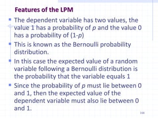
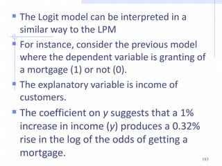
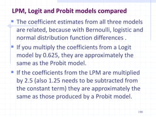
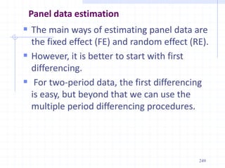
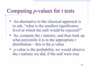
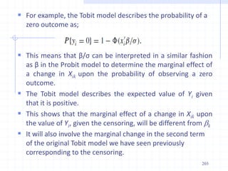
 The measured dependent variable of a decision maker are
assumed to be correlated with the latent variable through the
following threshold criterion
 Example: A working mother can establish just as warm and
secure of a relationship with her child as a mother who does
not work. [1=Strongly disagree; 2=Disagree; 3=Agree and
4=Strongly agree].
195

Other models with limited dependnet variables
Tobit Models
 The linear regression model assumes that the values
of all variables are continous and are observable
(known) for the entire sample.
 However, there are situations that the variables may
not be all observed for the entire sample.
 There are situations in which the sample is limited by
censoring or truncation.
 Censoring occurs when we observe the independent
variables for the entire sample, but for some
observations we have only limited information about
the dependent variable.
196

 In certain situations, the dependent variable
is continuous, but its range may be
constrained.
 Mostly, this occurs when the dependent
variable is zero for a substantial part of the
population but positive (with many different
outcomes) for the rest of the population.
 Examples: Amounts of credit, expenditures on
insurance, expenditures on durable goods,
hours of work on non-farm activities, and the
amount of FDI.
197

 Tobit models are particularly suited to model
these types of variables.
 The original Tobit model was suggested by James
Tobin (Tobin 1958), who analyzed household
expenditures on durable goods taking into
account their non-negativity.
 But only in 1964, Arthur Goldberger referred to
this model as a Tobit model, because of its
similarity to Probit models.
198

The Standard Tobit Model
 Suppose that we are interested in explaining the
expenditures on tobacco of households in a given
year.
 Let y denote the expenditures on tobacco, while z
denotes all other expenditures.
 Total disposable income (or total expenditures) is
denoted by x.
 We can think of a simple utility maximization
problem, describing the household’s decision
problem:
199

 We account for this by allowing for unobserved
heterogeneity in the utility function and thus for
unobserved heterogeneity in the solution as well. Thus
we write, where ε corresponds to
unobserved heterogeneity.
 If there were no restrictions on y and consumers could
spend any amount on tobacco, they would choose to
spend y∗.
 The solution to the original, constrained problem, will
therefore be given by
 So if a household would like to spend a negative
amount y∗, it will spend nothing on tobacco. 200

 This gives us the standard Tobit model, which we
formalize as follows.
 Notice the similarity of this model with the standard
probit model, the difference is in the mapping from
the latent variable to the observed variable.
 The above model is also referred to as the censored
regression model. It is a standard regression model,
where all negative values are mapped to zeros.
 That is, observations are censored (from below) at
zero. It also known as truncated regression model
201

 The model thus describes two things. One is the
probability that Yi = 0 (given Xi ), given by;
 The other is the distribution of Yi given that it is
positive. This is a truncated normal distribution with
expectation
 The last term in this expression denotes the conditional
expectation of a mean-zero normal variable given that it is
larger than −Xikb
 The coefficients in the Tobit model can be interpreted in a
number of ways, depending upon one’s interest. 202

 For example, the Tobit model describes the probability of a
zero outcome as;
 This means that β/σ can be interpreted in a similar fashion
as β in the Probit model to determine the marginal effect of
a change in Xik upon the probability of observing a zero
outcome.
 The Tobit model describes the expected value of Yi given
that it is positive.
 This shows that the marginal effect of a change in Xik upon
the value of Yi, given the censoring, will be different from bk
 It will also involve the marginal change in the second term
of the original Tobit model we have seen previously
corresponding to the censoring.
203

 It follows that the expected value of Yi is given by
 From this it follows that the marginal effect on the expected
value of Yi of a change in Xik is given by
Method of Estimation
 If we attempt with the OLS estimation, we cannot use the positive
observations Yi from the following model:
 Estimation of the Tobit model is usually done through maximum
likelihood.
204

 The contribution to the likelihood function of an
observation either equals the probability mass (at the
observed point Yi = 0) or the conditional density of Yi ,
given that it is positive, times the probability mass of
observing Yi > 0.
 Note that we have two sets of observations:
1.The positive values of y, for which we can write down
the normal density function as usual. We note that
has a standard normal distribution.
2.
205

Assumptions of Tobit Model
 There are two basic assumptions underlying the Tobit model.
1. The error term is not heteroskedastic.
2. The error term should have a normal distribution.
 If the error tem is either heteroskedastic or non-normally
distributed, then the maximum likelihood (ML) estimates are
inconsistent
206

 Basics:
Yt = b0 + b1 Yt-1 + b2 Yt-2+ . ..+ bk Yt-k + t
Whereas Yt-1, Yt-2+ . ..+ Yt-k Yt are
observations over the periods year 1, last year 2,
before last year, considered back.
 t is a noise process: homoscedastic and no
autocorrelation, this means t ~ IID (0, s2).
Chapter 7: Time Series Models
207

 Structural econometric modeling
 examines relationships between variables based
on economic theory
 useful in testing hypotheses, policy analysis
 less useful for forecasting if future values of
explanatory variables are missing
 Time series modeling
 detects past behavior of a variable to predict its
future
 popular as forecasting technique
 usually no underlying theory is involved or
considered. 208

 Time series data has a temporal
ordering, unlike cross-section data.
 We, thus, need to alter some of our
assumptions to take into account that we
no longer have a random sample of
individuals
 Instead, we have one realization of a
stochastic (i.e. random) process.
210

Examples of time series models
 A static model relates contemporaneous
variables: yt = b0 + b1 yt-1 + b2 yt-2 + ut
 This is known as finite distributed lag (FDL)
model
 A finite distributed lag (FDL) model allows
one or more variables to affect y with a lag
 More generally, a finite distributed lag
model of order q will include q lags of z
211

 Considering: yt = b0 + b1 yt-1 + b2 yt-2 + ut
 We can call b0 the impact propensity – it
reflects the immediate change in y
 For a temporary, 1-period change, y
returns to its original level in period q+1
 We can call b0 + b1 +…+ bq the long-
run propensity (LRP) – which reflects the
long-run change in y after a permanent
change.
212

Assumptions for unbiasedness
 Still we assume a model that is linear in
parameters: yt = b0 + b1xt1 + . . .+ bkxtk + ut
 And we need to make a zero conditional
mean assumption: E(ut|X) = 0, t = 1, 2, …, n
 Note that this implies the error term in any
given period is uncorrelated with the
explanatory variables in all time periods.
213

 This zero conditional mean
assumption implies the x’s are strictly
exogenous
 An alternative assumption, more
parallel to the cross-sectional case, is
E(ut|xt) = 0
 This assumption would imply the x’s
are contemporaneously exogenous
 But contemporaneous exogeneity will
only be sufficient in large samples
214

 Still we need to assume that no x is
constant, and that there is no perfect
collinearity
 Note we have skipped the assumption of
a random sample
 The key impact of the random sample
assumption is that each ui is independent
 Our strict exogeneity assumption takes
care of it in this case
215

 Based on these 3 assumptions, when using
time-series data, the OLS estimators are
unbiased
 Thus, just as was the case with cross-
section data, under the appropriate
conditions OLS is unbiased
 Omitted variable bias can be analyzed in
the same manner as in the cross-section
case
216

Variances of OLS estimators
 Just as in the cross-section case, we need
to add an assumption of homoskedasticity
in order to be able to derive variances
 Now we assume Var(ut|X) = Var(ut) = s2
 Thus, the error variance is independent of
all the x’s, and it is constant over time
 We also need the assumption of no serial
correlation: Corr(ut,us|X)=0 for t  s.
217

 Under these 5 assumptions, the OLS
variances in the time-series case are the
same as in the cross-section case.
 OLS remains BLUE
 With the additional assumption of normal
errors, inference is the same as the
procedures of making inference in cross
sectional data analysis.
218

Trending time series
 Time series data often have a trend
 Just because two or more series are
trending together, we can’t assume that
their relationship is causal.
 Often, both will be trending because of
other unobserved factors
 Even if those factors are unobserved, we
can control for them by directly
controlling for the trend
219

 One possibility is a linear trend, which can be
modeled as
yt = a0 + a1t + et, t = 1, 2, …
 Another possibility is an exponential trend,
which can be modeled as
log(yt) = a0 + a1t + et, t = 1, 2, …
 Another possibility is a quadratic trend, which
can be modeled as
yt = a0 + a1t + a2t2 + et, t = 1, 2, …
220

Seasonality
 Often time-series data exhibits some
periodicity, referred to seasonality
 Example: Quarterly data on retail sales will
tend to jump up in the 4th quarter
 Seasonality can be dealt with by adding a
set of seasonal dummies
 As with trends, the series can be seasonally
adjusted before running the regression
221

222
Stationarity
 Stationarity is an important property that must
hold before we can estimate a time-series
model, difficult to predict the future otherwise.
 A stochastic process is stationary if for every
collection of time indices 1 ≤ t1 < …< tm the joint
distribution of (xt1, …, xtm) is the same as that of
(xt1+h, … xtm+h) for h ≥ 1
 Thus, stationarity implies that the xt’s are
identically distributed and that the nature of any
correlation between adjacent terms is the same
across all periods.

224
Covariance stationary process
 If a process is non-stationary, we cannot use
its past structure to predict the future
 A stochastic process is covariance stationary if
E(xt) is constant, Var(xt) is constant and for any
t, h ≥ 1, Cov(xt, xt+h) depends only on h and not
on t
 Thus, this weaker form of stationarity requires
only that the mean and variance are constant
across time, and the covariance just depends
on the distance across time

225
Weakly Dependent Time Series
 A stationary time series is weakly
dependent if xt and xt+h are “almost
independent” as h increases
 If for a covariance stationary process
Corr(xt, xt+h) → 0 as h → ∞, this
covariance stationary process is said to be
weakly dependent
 We want to still use law of large numbers

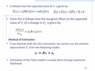
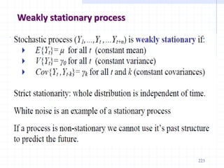
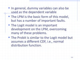
226
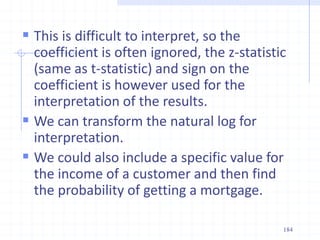
Types of the process
(a). Moving average (MA) process
 This process only assumes a relation between
periods t and t-1 via the white noise residuals et.
 A moving average process of order one [MA(1)]
can be characterized as one where
Yt = et + a1et-1, t = 1, 2,
with et being an iid sequence with mean 0 and
variance s2
 This is a stationary, weakly dependent sequence as
variables 1 period apart are correlated, but 2
periods apart they are not

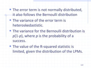
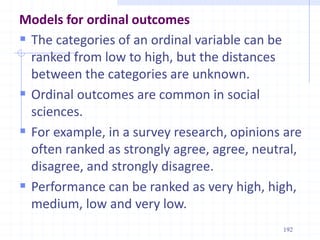
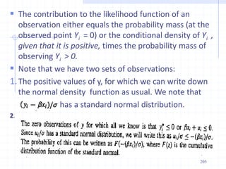
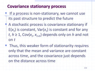
227
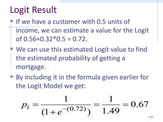
Autoregressive (AR) process
 An autoregressive process of order one
[AR(1)] can be characterized as one where
Yt = yt-1 + et , t = 1, 2,…
with et being an iid sequence with mean 0
and variance se
2
 For this process to be weakly dependent, it
must be the case that |r| < 1
 An autoregressive process of order one
[AR(p)]
Yt = 1 yt-1 + 2 yt-2 +… p yp-1 + et

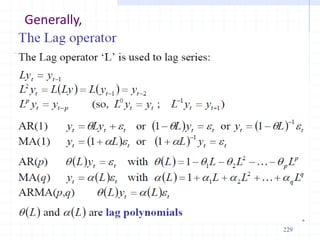
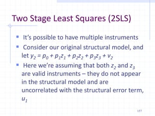
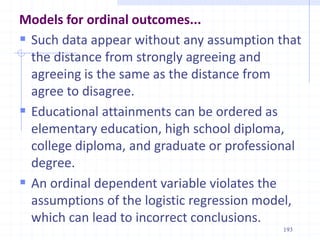
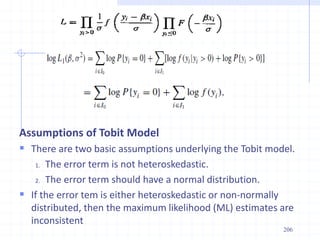
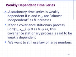
 Similarly, a moving average (MA) of order (q)]
can be given as
Yt = et + a1et-1 + a2et-2 + … + aqet-q
 A combined an AR(p) and MA(q) process can
be combined to an ARMA(p,q) process:
Yt = 1 yt-1 + 2 yt-2 + et + a1et-1 + a2et-2 … + aqet-q
 Using the lag operator:
LYt=Yt-1
L2Yt =L(L)Yt=L(Yt-1 )=Yt-2
LpYt =Yt-p
228

230
Assumptions for consistency
 Linearity and weak dependence
 A weaker zero conditional mean
assumption: E(ut|xt) = 0, for each t
 No perfect collinearity
 Thus, for asymptotic unbiasedness
(consistency), we can weaken the
exogeneity assumptions somewhat
relative to those for unbiasedness

231
Estimation and Inference for large sample
 Weaker assumption of homoskedasticity:
Var (ut|xt) = s2, for each t
 Weaker assumption of no serial
correlation: E(utus| xt, xs) = 0 for t  s
 With these assumptions, we have
asymptotic normality and the usual
standard errors, t statistics and F statistics
are valid.

232
Forecasting
 Once we’ve run a time-series regression
we can use it for forecasting into the future
 We can calculate a point forecast and
forecast interval in the same way we got a
prediction and prediction interval with a
cross-section
 Rather than using in-sample criteria like
adjusted R2, we often want to use out-of-
sample criteria to judge how good the
forecast is.

Summary of objectives and steps in time series analysis
233

Chapter 8: Panel Data Methods
234
 Basics
yit = b0 + b1xit1 + . . . bkxitk + uit
 A panel dataset contains observations on
multiple entities (individuals, companies…),
where each entity is observed at two or more
points in time.
 A panel of data consists of a group of cross-
sectional units (people, households, firms,
states, countries) who are observed over time.

 Panel data contains repeated observations of the
same cross-section unit.
 Hypothetical examples: Data on 20 Dire Dawa
schools in 2012 and again in 2017, for 40
observations total.
 Data on 9 Ethiopia Regional States, each state is
observed in 3 years, for a total of 27 observations.
 Data on 1000 individuals, in four different months,
for 4000 observations in total.
 Panel data estimation is often considered to be an
efficient analytical method in handling
econometric data.
235

1. Panel data can be used to deal with heterogeneity
in the micro units.
 Heterogeneity means that these micro units are
all different from one another in fundamental
unmeasured ways.
 Omitting these variables causes bias in estimation.
2. Panel data create more variability, through
combining variation across micro units with
variation over time, alleviating multicollinearity
problems.
 With this more informative data, more efficient
estimation is possible.
236

Advantages of Panel Data Regression
3. Panel data can be used to examine issues that cannot be
studied using time series or cross-sectional data alone.
4. Panel data allow better analysis of dynamic adjustment.
 Cross-sectional data can tell us nothing about dynamics.
 Time series data need to be very lengthy to provide good
estimates of dynamic behavior, and then typically relate
to aggregate dynamic behavior.
1. Long and narrow. With ‘‘long’’ describing the time
dimension and ‘‘narrow’’ implying a relatively small
number of cross sectional units.
Types of Panel Data
237

2. Short and wide. This type of panel data indicates that
there are many individuals observed over a relatively
short period of time
3. Long and wide. This type of data indicating that both
N and T are relatively large
4. Balanced Panel Data. These are data that do not have
any missing values or observations.
 It is the data in which the variables are observed for
each entity and for each time period.
5. Unbalanced Panel Data. These are data that have
some missing data for at least one time period for at
least one entity.
238

239
Pooled cross sections
 We may want to pool cross sections just to get bigger
sample sizes
 We may want to pool cross sections to investigate
the effect of time
 We may want to pool cross sections to investigate
whether relationships have changed over time
 Often loosely use the term panel data to refer to any
data set that has both a cross-sectional dimension
and a time-series dimension
 More precisely it’s only data following the same
cross-section units over time
 Otherwise it’s a pooled cross-section

240
Difference-in-Differences
 Say random assignment to treatment and
control groups, like in a medical
experiment
 One can then simply compare the change
in outcomes across the treatment and
control groups to estimate the treatment
effect
 For time 1,2, groups A, B
(y2,B – y2,A) - (y1,B – y1,A), or equivalently
(y2,B – y1,B) - (y2,A – y1,A), is the difference-
in-differences

241
 A regression framework using time and
treatment dummy variables can calculate this
difference-in-difference as well
 Consider the model:
yit = b0 + b1treatmentit + b2afterit + b3treatmentit*afterit + uit
 The estimated b3 is the difference-in-
differences in the group means

Example:
To evaluate whether a free school lunch service
improves outcomes of students, an experiment
is undertaken in Latin America. Student exam
(test) scores were collected from Rio and Sao
Paulo schools during the year 2008. Then,
students in Sao Paulo schools were provided
with free lunch services during the period 2009.
In 2010, students test scores were measured
from both Rio and Sao Paulo schools. The
measured results averaged from both sets of
schools before and after the free lunch service
are given below. 242

Example
Y
(Exam scores)
Pre
(2008)
Post
(2010)
Control
(Rio) 30 70
Treated
(Sao Paulo)
20 90
Question: What is the impact of the free lunch
program on student exam (test) scores?
243

 Difference in student exam (test) scores due
to time (D1) is:
D1 = 70 – 30 = 40
 Difference in student exam (test) scores due
to time and the free lunch program (D2) is:
D2 = 90 – 20 = 70
 Difference-in-difference or double difference
(DD) is:
DD = D2 – D1= 70 – 40 = 30
 Why is this?
244

Example: Two-observations over two periods
cases in general:
Y Dpost=0
(Pre)
Dpost=1
(Post)
Dtreatment = 0
(Control)
b0 b0b1
Dtreatment = 1
(Treated)
b0b2 b0b1 b2b3
245

Difference due to Time: D1
D1 = b0b1 b0 = b1
Difference due to Time and Treatment: D2
D2 = b0b1 b2b3 ) b0 b2  b1 b3
Difference-in-difference: DD
DD = D2 – D1= b1 b3 b1  b3
246

247
 When we don’t truly have random
assignment, the regression form becomes
very useful
 Additional x’s can be added to the
regression to control for differences across
the treatment and control groups
 Such cases are sometimes referred to as a
“natural experiment” especially when a
policy change is being analyzed

Econometrics1,2,3,4,5,6,7,8_ChaptersALL.pdf

Econometrics1,2,3,4,5,6,7,8_ChaptersALL.pdf

Recommended

Recommended

More Related Content

Similar to Econometrics1,2,3,4,5,6,7,8_ChaptersALL.pdf

Similar to Econometrics1,2,3,4,5,6,7,8_ChaptersALL.pdf (20)

Recently uploaded

Recently uploaded (20)

Econometrics1,2,3,4,5,6,7,8_ChaptersALL.pdf