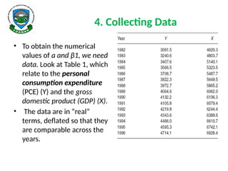
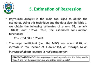
AAE 322: Econometrics
Topic 1: Introduction to Econometrics
1a: Purpose and Applications of Econometrics
WISDOM MGOMEZULU
What is econometrics
• Several working definitions:
1. “Econometrics is the interaction of economic
theory, observed data and statistical methods”
(Verbeek, 2008).
2. “Application of the mathematical statistics to
economic data in order to lend empirical support
to the economic mathematical models and
obtain numerical results” (Tintner, 1968)
What is Econometrics
3. “The quantitative analysis of actual economic
phenomena based on concurrent development
of theory and observation, related to approriate
methods of inference.” (Samuelson, et al., 1954)
4. “The social science in which the tools of
economic theory, mathematics, and statistical
inference are applied to the analysis of economic
phenomena” (Goldberger, 1964).
What is Econometrics:
Composite Definition
• Econometrics is all about:
– Considering economic theory;
– Collecting data; and
– Applying statistical tools on the data while testing
some hypotheses and draw some conclusions that
are helpful in policy making.
Why is Econometrics a Separate
Discipline?
• In other words, why is the study of these three
building blocks of econometrics (economic
theory, mathematics for economists, statisticts
for economists) individually not enough?
• Let’s look at the deficiencies of each of the
building blocks and how econometrics fills
those deficiencies.
Economic Theory
• Economic theory makes statements that are
mostly qualitative in nature (e.g. the law of
demand) without regard to any numerical
measure of the relationship.
– This is the job of econometrics, i.e. quantifying the
economic theory relationships.
Mathematical Economics
• The main concern of mathematical economics
is to express economic theory in mathematical
form without regard to measurability or
empirical verification of the theory.
– Econometrics is mainly interested in the empirical
verification of the economic theory models.
Statistics for Economists
• This is mainly concerned with collecting,
processing and presenting economic data in
form of charts and tables without necessarily
testing economic theories.
– Econometrics use collected data to test economic
theories
Methodology of Econometrics
• Traditional econometric methodology proceeds along
the following lines:
1. Statement of economic theory or hypothesis;
2. Specification of mathematical model of the theory;
3. Specification of the statistical, or econometric, model;
4. Collecting data;
5. Estimation of the parameters of the econometric model;
6. Hypothesis testing;
7. Forecasting and/or prediction; and
8. Using the model for policy purposes.
• The following example demonstrates the above
steps
1. Statement of Economic Theory
or Hypothesis
• Keynesian Theory states that ceteris paribus,
consumers increase their consumption as
their income increases, but not as much as the
increase in their income. (MPC < 1).
– MPC = marginal propensity to consume, i.e. rate of
change of consumption (say in $) by change in
income.
2. Specification of the Mathematical Model of
Consumption
Y = a + B1X (1)
Y = consumption expenditure (dependent variable)
X = income (dependent or explanatory variable)
a = intercept
B1 = coefficient
• The coefficient B1 measures the MPC
3. Specification of the Econometric
Model of Consumption
• The relationships between economic variables are generally
inexact. In addition to income, other variables affect
consumption expenditure, e.g. family size, age, education,
sex, etc.
• To allow for the inexact relationships between economic
variables, we add u (error term) to Equation (1) presented
earlier:
Y = a + B1X + u (2)
• The error term, among others, may represent those factors
that affect consumption but are not taken into account
explicitly.
4. Collecting Data
• To obtain the numerical
values of a and β1, we need
data. Look at Table 1, which
relate to the personal
consumption expenditure
(PCE) (Y) and the gross
domestic product (GDP) (X).
• The data are in “real”
terms, deflated so that they
are comparable across the
years.
5. Estimation of Regression
• Regression analysis is the main tool used to obtain the
estimates. Using this technique and the data given in Table 1,
we obtain the following estimates of a and β1, namely,
−184.08 and 0.7064. Thus, the estimated consumption
function is:
Yˆ = −184.08 + 0.7064Xi
• The slope coefficient (i.e., the MPC) was about 0.70, an
increase in real income of 1 dollar led, on average, to an
increase of about 70 cents in real consumption.
PRACTICE ASSIGNMENT: Use any computer package and enter the data given in
Table 1 and run the regression. Are you getting same results?
6. Hypothesis Testing
• That is to find out whether the estimates obtained are in
accordance with the expectations of the theory that is being
tested.
• Keynes expected the MPC to be positive but less than 1.
• In our example we found the MPC to be about 0.70. But
before we accept this finding as confirmation of Keynesian
consumption theory, we must enquire whether this estimate
is sufficiently below unity. In other words, is 0.70 statistically
less than 1? If it is, it may support Keynes’ theory. (This will be
covered in detail in the next topic, i.e. checking whether the
coefficient is significant or not).
7. Forecasting or Prediction
• To illustrate, suppose we want to predict the mean
consumption expenditure for 1997. The GDP value for 1997
was 7269.8 billion dollars consumption would be:
Yˆ1997 = −184.0779 + 0.7064 (7269.8) = 4951.3
PRACTICE ASSIGNMENT: Now suppose the government decides to propose a
reduction in the income tax. What will be the effect of such a policy on income
and thereby on consumption expenditure and ultimately on employment?
8. Use of the Model for Policy
Purposes
• Suppose we have the estimated consumption function given earlier. Suppose
further the government believes that consumer expenditure of about 4900 will
keep the unemployment rate at its current level of about 4.2%. What level of
income will guarantee the target amount of consumption expenditure?
• From the regression results, simple arithmetic will show that:
• 4900 = −184.0779 + 0.7064X
• which gives X = 7197, approximately. That is, an income level of about 7197
(billion) dollars, given an MPC of about 0.70, will produce an expenditure of about
4900 billion dollars.
• As these calculations suggest, an estimated model may be used for policy
purposes. By appropriate fiscal and monetary policy mix, the government can
manipulate the control variable X to produce the desired level of the target variable
Y.
Bibliography
• These lecture notes were prepared from various sources both
online and offline. The notable sources include:
1. https://www.slideshare.net/ishaqahmad22/econometrics-lecture-1s
t?from_action=save
(accessed: 1 May 2017)
2. https://www.slideshare.net/NiveditaSharma3/basic-econometrics-le
ctues1
(accessed 24 April 2017)
3. Verbeek, M. (2004). A Guide to Modern Econometrics. 2nd
Edition.
West Sussex, England: John Wiley and Sons Ltd.

Topic1a_purpose_and_applications_of_econometrics.pptx

  • 1.
    AAE 322: Econometrics Topic1: Introduction to Econometrics 1a: Purpose and Applications of Econometrics WISDOM MGOMEZULU
  • 2.
    What is econometrics •Several working definitions: 1. “Econometrics is the interaction of economic theory, observed data and statistical methods” (Verbeek, 2008). 2. “Application of the mathematical statistics to economic data in order to lend empirical support to the economic mathematical models and obtain numerical results” (Tintner, 1968)
  • 3.
    What is Econometrics 3.“The quantitative analysis of actual economic phenomena based on concurrent development of theory and observation, related to approriate methods of inference.” (Samuelson, et al., 1954) 4. “The social science in which the tools of economic theory, mathematics, and statistical inference are applied to the analysis of economic phenomena” (Goldberger, 1964).
  • 4.
    What is Econometrics: CompositeDefinition • Econometrics is all about: – Considering economic theory; – Collecting data; and – Applying statistical tools on the data while testing some hypotheses and draw some conclusions that are helpful in policy making.
  • 5.
    Why is Econometricsa Separate Discipline? • In other words, why is the study of these three building blocks of econometrics (economic theory, mathematics for economists, statisticts for economists) individually not enough? • Let’s look at the deficiencies of each of the building blocks and how econometrics fills those deficiencies.
  • 6.
    Economic Theory • Economictheory makes statements that are mostly qualitative in nature (e.g. the law of demand) without regard to any numerical measure of the relationship. – This is the job of econometrics, i.e. quantifying the economic theory relationships.
  • 7.
    Mathematical Economics • Themain concern of mathematical economics is to express economic theory in mathematical form without regard to measurability or empirical verification of the theory. – Econometrics is mainly interested in the empirical verification of the economic theory models.
  • 8.
    Statistics for Economists •This is mainly concerned with collecting, processing and presenting economic data in form of charts and tables without necessarily testing economic theories. – Econometrics use collected data to test economic theories
  • 9.
    Methodology of Econometrics •Traditional econometric methodology proceeds along the following lines: 1. Statement of economic theory or hypothesis; 2. Specification of mathematical model of the theory; 3. Specification of the statistical, or econometric, model; 4. Collecting data; 5. Estimation of the parameters of the econometric model; 6. Hypothesis testing; 7. Forecasting and/or prediction; and 8. Using the model for policy purposes. • The following example demonstrates the above steps
  • 10.
    1. Statement ofEconomic Theory or Hypothesis • Keynesian Theory states that ceteris paribus, consumers increase their consumption as their income increases, but not as much as the increase in their income. (MPC < 1). – MPC = marginal propensity to consume, i.e. rate of change of consumption (say in $) by change in income.
  • 11.
    2. Specification ofthe Mathematical Model of Consumption Y = a + B1X (1) Y = consumption expenditure (dependent variable) X = income (dependent or explanatory variable) a = intercept B1 = coefficient • The coefficient B1 measures the MPC
  • 12.
    3. Specification ofthe Econometric Model of Consumption • The relationships between economic variables are generally inexact. In addition to income, other variables affect consumption expenditure, e.g. family size, age, education, sex, etc. • To allow for the inexact relationships between economic variables, we add u (error term) to Equation (1) presented earlier: Y = a + B1X + u (2) • The error term, among others, may represent those factors that affect consumption but are not taken into account explicitly.
  • 13.
    4. Collecting Data •To obtain the numerical values of a and β1, we need data. Look at Table 1, which relate to the personal consumption expenditure (PCE) (Y) and the gross domestic product (GDP) (X). • The data are in “real” terms, deflated so that they are comparable across the years.
  • 14.
    5. Estimation ofRegression • Regression analysis is the main tool used to obtain the estimates. Using this technique and the data given in Table 1, we obtain the following estimates of a and β1, namely, −184.08 and 0.7064. Thus, the estimated consumption function is: Yˆ = −184.08 + 0.7064Xi • The slope coefficient (i.e., the MPC) was about 0.70, an increase in real income of 1 dollar led, on average, to an increase of about 70 cents in real consumption. PRACTICE ASSIGNMENT: Use any computer package and enter the data given in Table 1 and run the regression. Are you getting same results?
  • 15.
    6. Hypothesis Testing •That is to find out whether the estimates obtained are in accordance with the expectations of the theory that is being tested. • Keynes expected the MPC to be positive but less than 1. • In our example we found the MPC to be about 0.70. But before we accept this finding as confirmation of Keynesian consumption theory, we must enquire whether this estimate is sufficiently below unity. In other words, is 0.70 statistically less than 1? If it is, it may support Keynes’ theory. (This will be covered in detail in the next topic, i.e. checking whether the coefficient is significant or not).
  • 16.
    7. Forecasting orPrediction • To illustrate, suppose we want to predict the mean consumption expenditure for 1997. The GDP value for 1997 was 7269.8 billion dollars consumption would be: Yˆ1997 = −184.0779 + 0.7064 (7269.8) = 4951.3 PRACTICE ASSIGNMENT: Now suppose the government decides to propose a reduction in the income tax. What will be the effect of such a policy on income and thereby on consumption expenditure and ultimately on employment?
  • 17.
    8. Use ofthe Model for Policy Purposes • Suppose we have the estimated consumption function given earlier. Suppose further the government believes that consumer expenditure of about 4900 will keep the unemployment rate at its current level of about 4.2%. What level of income will guarantee the target amount of consumption expenditure? • From the regression results, simple arithmetic will show that: • 4900 = −184.0779 + 0.7064X • which gives X = 7197, approximately. That is, an income level of about 7197 (billion) dollars, given an MPC of about 0.70, will produce an expenditure of about 4900 billion dollars. • As these calculations suggest, an estimated model may be used for policy purposes. By appropriate fiscal and monetary policy mix, the government can manipulate the control variable X to produce the desired level of the target variable Y.
  • 18.
    Bibliography • These lecturenotes were prepared from various sources both online and offline. The notable sources include: 1. https://www.slideshare.net/ishaqahmad22/econometrics-lecture-1s t?from_action=save (accessed: 1 May 2017) 2. https://www.slideshare.net/NiveditaSharma3/basic-econometrics-le ctues1 (accessed 24 April 2017) 3. Verbeek, M. (2004). A Guide to Modern Econometrics. 2nd Edition. West Sussex, England: John Wiley and Sons Ltd.

Editor's Notes

  • #18 https://www.slideshare.net/ishaqahmad22/econometrics-lecture-1st?from_action=save