This document presents a dynamical model of a vibrocompactor used in railroad construction. The model represents the vibrocompactor as a two-mass mechanical system with two degrees of freedom. Differential equations are derived to describe the forced vibrations of the system excited by an inertial disturbance. Numerical analysis is performed to examine the system's behavior under different forcing frequencies, including its natural frequencies and frequency response. The results indicate the machine can operate steadily over a wide range of frequencies except near its first natural frequency, where non-stationary beating vibrations occur.

1. IOSR Journal of Mechanical and Civil Engineering (IOSR-JMCE)
e-ISSN: 2278-1684,p-ISSN: 2320-334X, Volume 12, Issue 6 Ver. VI (Nov. - Dec. 2015), PP 01-05
www.iosrjournals.org
DOI: 10.9790/1684-12660105 www.iosrjournals.org 1 | Page
Vibrations of a mechanical system with inertial and forced
disturbance
Boris Petkov, PhD
(Department of Material Handling and Construction Machines, University of Transport “T. Kableshkov”, Sofia,
Bulgaria)
Abstract: We present a mechanical system model of the inertial type vibrocompactor used in railroad building.
In the paper we examine forced vibrations of the mechanical system excited by inertial disturbance. Using a
dynamical model of the mechanical system and applying numerical methods, frequency response and frequency
relations are found.
Keywords: vibrocompactor, dynamical model, frequency response, inertial forced vibrations.
I. Introduction
Vibrocompacting of bulk materials is widely used in the construction, repair, and maintenance of
automobile and rail-roads. This ensures that the road’s overlays are dense enough for the needed strength of the
road.
Vibrocompacting is a dynamic process that creates a specific level of density of the bulk materials
through regulating the different parameters — frequency, amplitude, and force/pressure.
The dynamical modelling of the vibrating machine of inertial type enables to study working regimes
depending on different frequencies of disturbance action.
The results of the study of the dynamical model are vital in the construction of vibrocompactors.
II. Dynamical model
The inertial vibrocompactor can be represented as a two-mass system (Fig. 1) with two degrees of
freedom, that performs forced oscillations generated by an inertial disturbance [1]. The parameters of the system
are focused — it has been assumed that the motion is only along one of the principal axes.
Fig.1. Dynamical model of a vibrocompactor of inertial type
The second kind Lagrange equation is used to describe the forced fluctuations from the stable state of
the mechanical system in the presence of potential and dissipative forces.
The system of differential equations, describing the model, follows:
zxxx

 CBM (1)

2. Vibrations of a mechanical system with inertial and forced disturbance
DOI: 10.9790/1684-12660105 www.iosrjournals.org 2 | Page
where:
  






2
1
0
0
m
m
M   








22
221
bb
bbb
B   








22
221
cc
ccc
C 






F
tsinP 
z

III. Natural frequencies and frequency response
1. The natural frequencies are determined for the free vibrations of the undamped system [2]:
0 xCxM

(2)
The harmonic solutions for x mean that it has the form x = Xsinωt and substitution into the equation of
motion (2) gives:
  02
 XCM (3)
The natural frequencies are found by solving the eigenvalue problem:
  0det  MC  , where λ = ω2
(λ>0, λR). (4)
The natural frequencies follow as ii   .
Using MATLAB and the values of the parameters listed in the appendix, the following natural
frequencies are calculated:
ω1 = 138.8 s-1
and ω2 = 929.5 s-1
.
2. Frequency response is determined for the forced damped system [2] after a Laplace transformation of
equation (1) has been performed:
     ssss2
zXCBM  or      ssss
12
zCBMX

 , where s = iω and therefore:
      iii
12
zCBMX

 (5)
The frequency response function (fig.2) is built using (5) in MATLAB.
0 100 200 300 400 500 600 700 800 900 1000
0
0.1
0.2
0.3
0.4
0.5
0.6
0.7
0.8
0.9
1
omega
X
Fig.2 Frequency response of the damped system
IV. Numerical analysis
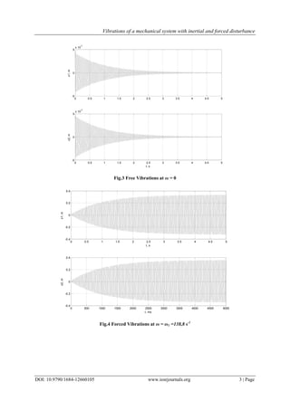
We show the numerical analysis of the system for four cases: free vibrations (ω = 0), dynamic
multiplication (ω = ω1, ω = ω2), beating regime (ω is close to ω1) and regime with frequency inbetween
natural frequencies [3].
The numerical solutions are found in MATLAB (see the values of machine’s parameters are in the appendix).

3. Vibrations of a mechanical system with inertial and forced disturbance
DOI: 10.9790/1684-12660105 www.iosrjournals.org 3 | Page
0 0.5 1 1.5 2 2.5 3 3.5 4 4.5 5
-5
0
5
x 10
-3
x1,m
0 0.5 1 1.5 2 2.5 3 3.5 4 4.5 5
-5
0
5
x 10
-3
t, s
x2,m
Fig.3 Free Vibrations at ω = 0
0 0.5 1 1.5 2 2.5 3 3.5 4 4.5 5
-0.4
-0.2
0
0.2
0.4
t, s
x1,m
0 500 1000 1500 2000 2500 3000 3500 4000 4500 5000
-0.4
-0.2
0
0.2
0.4
t, ms
x2,m
Fig.4 Forced Vibrations at ω = ω1 =138,8 s-1

4. Vibrations of a mechanical system with inertial and forced disturbance
DOI: 10.9790/1684-12660105 www.iosrjournals.org 4 | Page
0 0.5 1 1.5 2 2.5 3 3.5 4 4.5 5
-0.1
-0.05
0
0.05
0.1x1,m
0 0.5 1 1.5 2 2.5 3 3.5 4 4.5 5
-0.1
-0.05
0
0.05
0.1
t, s
x2,m
Fig.5 Forced Vibrations at ω = ω2 =929,5 s-1
0 0.5 1 1.5 2 2.5 3 3.5 4 4.5 5
-0.04
-0.02
0
0.02
0.04
x1,m
0 0.5 1 1.5 2 2.5 3 3.5 4 4.5 5
-0.04
-0.02
0
0.02
0.04
t, s
x2,m
Fig.6 Forced Vibrations at ω =130 s-1
(close to ω1)

5. Vibrations of a mechanical system with inertial and forced disturbance
DOI: 10.9790/1684-12660105 www.iosrjournals.org 5 | Page
0 0.5 1 1.5 2 2.5 3 3.5 4 4.5 5
-0.03
-0.02
-0.01
0
0.01
0.02
0.03
x1,m
0 0.5 1 1.5 2 2.5 3 3.5 4 4.5 5
-0.03
-0.02
-0.01
0
0.01
0.02
0.03
t, s
x2,m
Fig.7 Forced Vibrations at ω = 400 s-1
In all cases, during the stationary regime, there are steady harmonic vibrations. At frequencies 130 s-1
and 400 s-1
(fig. 6, fig. 7) the non- stationary processes are poly harmonic duе to the beat on both coordinates
x1 and x2.
V. Conclusions
The examination of vibrations of the inertial type vibrocompactor prove that the machine can work
steady and properly inside a wide range of frequencies except these ones in the area near the first natural
frequency where the beat breaks up steady work in non- stationary regimes.
Such examination could take part in the process of constructing of new machines or improve the
performance of the existing ones.
Appendix
Parameter Value dimension Parameter Value dimension
Mass of vibrator incl. unbalanced
mass – m1
40 kg Damping coefficient of the
gravel – b2
1900 Ns/m
Mass of the tampers – m2 60 kg Damping coefficient of the
suspension – b1
200 Ns/m
Stiffness coefficient of the suspension
– c1
2.106
N/m Force - F 10 kN
Stiffness coefficient of the gravel – c2 21.106
N/m Radius of the unbalanced
mass - r
0.05 m
References
[1]. B. Petkov, Dynamic model of vibrocompactor with two degrees of freedom, Mechanics, Transport, Communications:3-2015.
[2]. Тондл А., Нелинейные колебания механических систем,( Мир, Москва, 1978)
[3]. D. Vasilev, Vibrations of a mechanical system with positional dry friction and kinematics and forced disturbance, Mechanics,
Transport, Communications:3-2015.