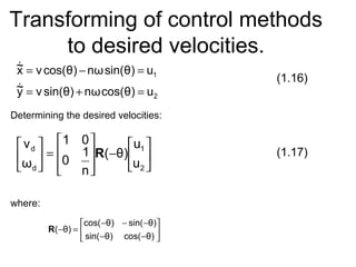
This thesis proposes a control system for generating control rules to dynamically manage a mobile robot. The objective is to model a control system that determines the robot's behavior based on its movement and environmental changes. Methods include using dynamical models, kinematic models, and hybrid systems to transform control methods into desired velocities. Experiments were conducted to test the system with obstacles. Results showed the selected synthetic approaches suitably achieved position control objectives. The thesis purpose of synthesizing a mobile robot control system was successfully achieved, validated by dynamic simulation of the management system.

2. Thesis:
Synthesis of control of mobile robot with dynamic
system for generating of control rules.
Made by: Hristo Ganchev
Major: AICT
Technical University Sofia–
Branch Plovdiv

3. Objective:
• The aim of the thesis is to model
management system for a mobile robot
through dynamic assignments that
determine the behavior of mobile robot at
a certain movement and changes in the
environment.

4. Methods used to achieve the target :
lllr
rrlr
θkMθaθb
θkMθbθa


−=+
−=+
Dynamical model:
(1.2)
i
ii
Q=
q
L
-
q
L
dt
d
∂
∂






∂
∂

(1.1)
Is transforming to:
τ=+ ωKωH fc

Transformation into Hamilton equation:
(1.3)
Transformation of the speed:
ωθ,ωθ,ωθ,ωθ,ωθ llllrrrr ===== 
Oyler- Lagrange:

5. ωθ
)θsin(vy
)θcos(vx
=
=
=



(1.4)
R2
ωlv2
ω
R2
ωlv2
ω
l
r
−
=
+
=
( ) )θcos(ωω
2
R
x lr +=
( ) )θsin(ωω
2
R
y lr +=
( )lr ωω
l
R
θ −=
(1.6)
(1.5)
„Unicycle“ model:
Differential mobile robot:
Connection between the speed:
Kinematic model:

6. Generating the references of control
behaviors:
u
p
Fig.1 Point behavior
px
px
2
1
=
= (1.9)
(1.8)
(1.7)
(1.10)
ux
xx
2
21
=
=


u
1
0
x
x
00
10
u
x
2
12






+











=





=x
Cxy
BuAxx
=
+=
State variables: Vector matrix :
Dynamic of state variables: Stationary sistem:

7. x
xg
Fig.2 Go to goal behavior.
Control law:
gtggtggtg eKu = (1.11)
u
uxx 





+





=
10
01
00
00

Go to goal.

8. xo
x
Fig.3 Avoiding obstacles behavior.
Control law:
aoaoao eKu = (1.12)
Avoiding obstacle:

9. Δ
.. xo
uao
ucfw
uccfw
Fig.4 “Follow the wall” behavior.

10. aoaoaocfw u
2
π
αu
2
π
cos
2
π
sin
2
π
sin
2
π
cos
αu
01
10
αu 





−=


















−





−






−−





−
=





−
= R
aoaoaoccfw u
2
π
αu
2
π
cos
2
π
sin
2
π
sin
2
π
cos
αu
01
10
αu 





=






























−





=




 −
= R
where R is the rotational matrix which have to make the following the wall to be at
semicircle instead of line and α is constant which limiting the length of vector u.
(1.13b)
(1.13a)
Control methods for “follow the wall”
behavior:
Clockwise follow:
Counterclockwise follow:

11. Δ
xo
uao
ucfw
ugtg
uccfw
xg
Determining the direction is made from the product between vector of following
wall and the vector of go to goal behaviors.
( ))u,u(cosuuuuu,u ccfwgtgccfwgtgccfw
T
gtgccfwgtg ∠==
ccfwccfwgtg u0u,u ⇒>
Fig. 5 Determine the direction of “following wall”
(1.14a)
(1.14b)

12. Hybrid system:
Fig. 6

13. )cos()sin(~
)sin()cos(~
θωθ
θωθ
nvy
nvx
+=
−=


(1.15)
Dynamic of new point:
Fig.7

14. Transforming of control methods
to desired velocities.
2
1
u)θcos(ωn)θsin(vy~
u)θsin(ωn)θcos(vx~
=+=
=−=








−








=





2
1
d
d
u
u
)θ(
n
1
0
01
ω
v
R






−−
−−−
=−
)θcos()θsin(
)θsin()θcos(
)θ(R
Determining the desired velocities:
where:
(1.16)
(1.17)

15. Linearization of dynamic:
τBAωω +=
1
fc
1
HB
KHA
−
−
=
−=
mmm BRAωω τr+=
Motor shaft transformation:
където :
Final equation:
ττ
τ
τ
τ
τ
m r
1
r m =⇒=ωrω
r
1
ω
ω
ωm
ωm
=⇒=
τrrr ω=
където : 





=
r0
0r
rR
(1.18)
(1.19)
(1.21)
Total ratio:
(1.20)
Dynamic of wheel velocities:

16. Cascade System for management
speeds of the mobile robot :
Fig.8

17. Overall management system of
mobile robot :
Fig.9

18. Experiment data :
xg,
[m]
yg,
[m]
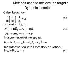
Δ, [m] ε, [m] Tf, [s] ti kp xo,
[m]
yo,
[m]
5 5 0.3 0.05 80 0.001 1 1.4 1.5
Table 1
Test 1. Coordinate system motion with one obstacle in the
way of the robot.

19. 0 0.5 1 1.5 2 2.5 3 3.5 4 4.5 5
0
0.5
1
1.5
2
2.5
3
3.5
4
4.5
5
x, [m]
y,[m]
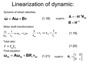
Fig.10
Trajectory in coordinate system

20. 0 10 20 30 40 50 60 70 80
-5
0
5
10
15
20
25
t,[s]
wr
,wrd
[rad/s]
Желана ъглова скорост на дясното колело
Ъглова скорост на дясното колело
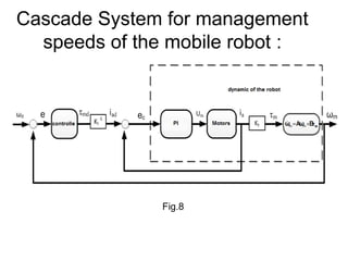
Fig.11
0 10 20 30 40 50 60 70 80
-5
0
5
10
15
20
25
t,[s]
wl
,wld
[rad/s]
Желана ъглова скорост на лявото колело
Ъглова скорост на лявото колело
Angular velocities of right and left
wheels:

21. 0 10 20 30 40 50 60 70 80
-3
-2
-1
0
1
2
3
x 10
-3
t,[s]
Mr
,Mrd
,[Nm]
Желан момент на десния двигател
Момент на десния двигател
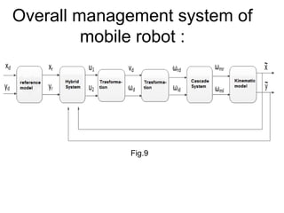
Fig.12
0 10 20 30 40 50 60 70 80
-2.5
-2
-1.5
-1
-0.5
0
0.5
1
1.5
2
x 10
-3
t,[s]
Ml
,Mld
,[Nm]
Желан момент на левия двигател
Момент на левия двигател
Torques of right and left motors

22. 0 10 20 30 40 50 60 70 80
-0.4
-0.3
-0.2
-0.1
0
0.1
0.2
0.3
t,[s]
iar
,iard
[A]
Желан ток на десния двигател
Ток на десния двигател
Fig.13
0 10 20 30 40 50 60 70 80
-0.25
-0.2
-0.15
-0.1
-0.05
0
0.05
0.1
0.15
0.2
t,[s]
ial
,iald
[A]
Желан ток на левия двигател
Ток на левия двигател
Right and left motor currents:

23. xg,
[m]
yg,
[m]
Δ,
[m]
ε,
[m]
Tf,
[s]
ti kp xo,
[m]
yo,
[m]
xo2,
[m]
yo2,
[m]
5 5 0.3 0.05 100 0.001 0.5 1.4 1.5 3.2 2.9
Table 2
Test 2. Coordinate system motion
with two obstacles in the way of the
robot.

24. 0 0.5 1 1.5 2 2.5 3 3.5 4 4.5 5
0
0.5
1
1.5
2
2.5
3
3.5
4
4.5
5
Траектория на мобилния робот в координатната система
x, [m]
y,[m]
Fig.14 Trajectory

25. 0 10 20 30 40 50 60 70 80 90 100
-5
0
5
10
15
20
25
t,[s]
wr
,wrd
[rad/s]
Желана ъглова скорост на дясното колело
Ъглова скорост на дясното колело
Fig.15
0 10 20 30 40 50 60 70 80 90 100
-5
0
5
10
15
20
25
t,[s]
wl
,wld
[rad/s]
Желана ъглова скорост на лявото колело
Ъглова скорост на лявото колело
Angular velocities of right and left
wheels:

26. 0 10 20 30 40 50 60 70 80 90 100
-6
-5
-4
-3
-2
-1
0
1
2
3
x 10
-3
t,[s]
Mr
,Mrd
,[Nm]
Желан момент на десния двигател
Момент на десния двигател
0 10 20 30 40 50 60 70 80 90 100
-3
-2
-1
0
1
2
3
4
5
6
x 10
-3
t,[s]
Ml
,Mld
,[Nm]
Желан момент на левия двигател
Момент на левия двигател
Fig.16
Torques of right and left motors

27. 0 10 20 30 40 50 60 70 80 90 100
-0.5
-0.4
-0.3
-0.2
-0.1
0
0.1
0.2
0.3
t,[s]
iar
,iard
[A]
Желан ток на десния двигател
Ток на десния двигател
Фиг.17
0 10 20 30 40 50 60 70 80 90 100
-0.3
-0.2
-0.1
0
0.1
0.2
0.3
0.4
0.5
0.6
t,[s]
ial
,iald
[A]
Желан ток на левия двигател
Ток на левия двигател
Right and left motor currents:

28. Conclusions:
 A study of the behavior of the closed nonlinear system shows that the
selected synthetic approaches to system positional control of wheeled
mobile robot suitable for achieving the desired objectives of
management.
 Based on the results it can be argued that the purpose of the thesis -
synthesis of managing mobile robot is successfully executed, the
results obtained are appropriate and validated by dynamic simulation
management system.

29. Thanks!