SPSS GuideAssessing Normality, Handling Missing Data, and Calculating Scores.pdf

Missing Data
Missing data is a common issue in research that occurs when there are gaps or omissions in the
collected data
Types of Missing Data:
Missing Completely at Random (MCAR): Data is MCAR when the likelihood of missingness is the
same for all units. In other words, it's purely random. There's no rela onship between the
missingness of the data and any values, observed or unobserved.
Missing at Random (MAR): Data is MAR if the likelihood of missingness is the same only within
groups defined by the observed data. Meaning, once you control for other variables in your dataset,
the data missingness is random. There may be a systema c rela onship between the propensity of
missing values and the observed data, but not the missing data.
Example
Imagine you conducted a survey asking about people's income and age. Some people might not feel
comfortable sharing their income, and so they leave that ques on unanswered. But, suppose you
no ce that younger people (for example, people aged 18-25) are more likely to leave the income
ques on blank compared to older age groups.
In this case, the data is "Missing at Random" (MAR). The missing data (income) is related to some of
the observed data (age group), but within those age groups, the missingness is random.
So, when we say data is MAR, we mean that missingness can be explained by other informa on we
have in the data set (like age), but not by the missing data itself. In other words, if we consider age,
the likelihood of income being missing is the same across all income levels.
Missing Not at Random (MNAR): If neither MCAR nor MAR holds, the missing data is MNAR. That is,
the missingness depends on informa on not available in your data.
Example
Imagine you're conduc ng a survey asking people about their salary. But, some people with very
high or very low salaries might not want to reveal their salary, so they leave the ques on blank. Here,
the missingness (the lack of salary informa on) is directly related to the missing data itself (the
actual salary amount).
In this case, we say the data is "Missing Not at Random" (MNAR). This means that there is a specific
reason related to the missing informa on itself that it's missing. We can't predict or explain the
missingness using the other informa on we have in our survey because it's not about their age,
gender, loca on or any other factor we've recorded. It's about the missing informa on itself.
So, in MNAR, the fact that data is missing is directly connected to the data itself, and it's not just
random or connected to other, known data. This can make it tricky to deal with in analysis because
we don't have any observed data to help us account for the missingness
Effects of Missing Data:
Missing data can lead to a loss of sta s cal power, introduce bias and make the handling and analysis
of the data more arduous.

Handling Missing Data:
Listwise Dele on (Complete-Case Analysis): In this method, you remove any case with at least one
missing value. This method is straigh orward but can lead to a significant loss of data, especially if
the missingness is extensive.
Pairwise Dele on: Here, the analysis is done on all cases in which the variables of interest are
present. It is more efficient in using available data than listwise dele on but can complicate the
analysis, his method works by using all of the available data for each calcula on or analysis that is
done. It does not delete any informa on unless it's necessary for a specific calcula on.
Example
Imagine you're studying the rela onship between three variables - age, income, and educa on level -
using a survey data. You have a sample size of 1000 respondents. Some respondents didn't provide
their income, others didn't provide their educa on level, but all respondents provided their age.
If you're analyzing the rela onship between age and income, you'll only exclude the respondents
who did not provide their income, and you use all the remaining data.
Similarly, when you're analyzing the rela onship between age and educa on level, you'll only
exclude the respondents who did not provide their educa on level, and use all the remaining data.
So, in both these analyses, you're only excluding the "pair" of data points that are not available, and
using all the remaining data - hence the term "pairwise dele on."
This method is good because it uses as much data as possible, allowing you to keep the power of
your analysis high. However, it can complicate the analysis, especially when missingness is not
random and if the missing data pa erns differ across different variable pairs, which could poten ally
lead to bias or inconsistent results.
Imputa on: This involves filling in the missing values with es mates. The simplest form of this is
mean/mode/median imputa on, where the missing values are replaced with the
mean/mode/median of the available cases
Mul ple Imputa on: An extension of the above approach, this involves crea ng mul ple imputed
datasets, analyzing each one separately, and then pooling the results to create a single es mate. This
method helps to capture the uncertainty around the missing values.
Example
Suppose you're a project manager overseeing several ongoing projects within your company. You are
analyzing data on project dura on, cost, team size, and project success rate to iden fy key factors
impac ng the efficiency and success of projects.
However, some of the projects in your dataset are s ll ongoing, meaning you have missing data for
the 'project dura on' and 'project success rate' fields.
Step 1: Ini al Imputa on
You first use the available data to es mate the missing values. You might use a regression model
using 'team size' and 'cost' as predictors to es mate 'project dura on'. This provides you with one
complete dataset.

Step 2: Mul ple Imputa ons
Next, instead of es ma ng the missing data just once, you repeat the process mul ple mes (let's
say 5 mes), each me adding some random varia on to your es mates. This gives you five different
complete datasets, each slightly different due to the added random noise.
Step 3: Analysis
You analyze each of these five datasets independently, assessing the influence of dura on, cost, and
team size on the success of projects.
Step 4: Pooling the results
Finally, you combine the results from the five separate analyses into a single result. Techniques like
Rubin's rules are used to account for the variability between the imputa ons.
This mul ple imputa on process provides a more robust and valid analysis of project outcomes, even
in the presence of missing data. It also acknowledges the uncertainty surrounding the es ma on of
the missing project dura ons and success rates.
So, in short, mul ple imputa on is a process where you make educated guesses to fill in missing
data, do this mul ple mes to acknowledge uncertainty, then analyze each guess and average the
results. This gives you a more robust and reliable result when dealing with missing data.
Imputa on: This involves filling in the missing values with es mates. The simplest form of this is
mean/mode/median imputa on, where the missing values are replaced with the
mean/mode/median of the available cases.
Mul ple Imputa on: An extension of the above approach, this involves crea ng mul ple imputed
datasets, analyzing each one separately, and then pooling the results to create a single es mate. This
method helps to capture the uncertainty around the missing values.
Model-based methods: These are more sophis cated sta s cal techniques, such as maximum
likelihood es ma on or Bayesian methods, that use all the observed data to es mate a sta s cal
model.
Listwise or Pairwise Dele on: This is SPSS's default method. In Listwise dele on, SPSS
automa cally excludes cases (rows) with missing values in any variable from the analysis. In
Pairwise dele on, SPSS uses all cases with valid (non-missing) values for the par cular pairs
of variables being analyzed. You don't have to do anything to implement these - SPSS will do
it automa cally.
Mul ple Imputa on: SPSS has a built-in mul ple imputa on feature you can use to handle
missing data more robustly. Here's how(Not in spss),there is another method there not
accurate is EM("Expecta on-Maximiza on")
es mates the missing data and the maximiza on step (M-step) re-es mates the parameters
using the completed data. This process con nues un l convergence.

ASSESSING NORMALITY
.assessing normality is like making sure you're using the right recipe for what you're cooking. If you're
baking cookies, but use a recipe for a cake, things might not turn out well. Similarly, understanding if
your data follows a normal distribu on helps you use the right sta s cal techniques, so your
conclusions are meaningful and accurate.
why we need to check for this:
 Many Methods Rely on It: A lot of the techniques we use in sta s cs assume that the data
follows this bell-shaped pa ern. If the data doesn't follow this pa ern, the results of our
analysis could be misleading or incorrect.
 It Helps Us Make Predic ons: If we know that our data follows this normal distribu on
pa ern, we can make predic ons and conclusions that are usually reliable. It's like knowing
the rules of a game; once you know them, you can play eﬀec vely.
 Understanding the Data Be er: By checking if our data follows this pa ern, we can be er
understand how our data behaves. It helps us see if most of our data falls near the average
or if there are lots of extreme values.
 Choosing the Right Tools: If the data doesn't follow this pa ern, we may need to use
diﬀerent sta s cal methods that don't rely on this assump on. It's like using the right tool
for the job; you need to
how you can assess normality:
Several techniques can be used to assess normality, both graphically and through sta s cal tests.
Here, we'll explore the graphical methods:
 Histogram: A histogram represents the distribu on of data by forming bins along the range
of the data and then drawing bars to show the number of observa ons in each bin. A bell-
shaped histogram indicates normality.
 a normally distributed dataset
the classic bell-shaped curve,
indica ng a normal distribu on.
Non-Normally Distributed Data

Q-Q Plot (Quan le-Quan le Plot): This plot helps us compare two probability distribu ons
by plo ng their quan les against each other. If the data is normally distributed, the points in
the Q-Q plot will approximately lie along a straight line.
Box Plot: A box plot can provide a visual representa on of the distribu on's central tendency
and spread. It won't exactly tell you if the data is normally distributed, but extreme skewness
or many outliers can be an indica on that the data is not normal.
Q-Q Plot: Points deviate from the straight
line, especially at the ends, indica ng non-
normality
No signiﬁcant skewness or outliers
are visible, consistent with a normal
distribu on

Interpretation of output from Explore
how the concepts I described relate to normality
 Mean, Median, and Mode: In a perfectly normal distribu on, these three measures
coincide. If they are significantly different, it may suggest a skewness in the
distribu on.
 Standard Devia on: This sta s c tells us about the spread or dispersion of the data.
In a normal distribu on, about 68% of the data will fall within one standard
devia on of the mean, 95% within two standard devia ons, and 99.7% within three
standard devia ons. Devia ons from this pa ern can indicate non-normality.
 Trimmed Mean: If there's a significant difference between the original mean and the
5% trimmed mean, it may indicate the presence of outliers, which can distort the
normality of a distribu on.
 Extreme Values and Outliers: These can heavily influence the mean and standard
devia on, making a distribu on appear more skewed or fla ened than it would
without these values. Extreme values might need to be inves gated further, as they
can indicate non-normality in the data.
 95% Confidence Interval: While not a direct test of normality, understanding the
range in which the true popula on mean is likely to lie can be informa ve, especially
if you are using methods that assume normality.
If normality is a cri cal assump on for your analysis (as it is for many parametric sta s cal
tests), you may wish to conduct a formal test for normality, such as the Shapiro-Wilk test, the
Anderson-Darling test, or the Kolmogorov-Smirnov test, depending on your specific situa on
and data size.
Let's break down the Mean, Median, Mode, and Standard Devia on, and discuss their
rela onship to normality.
Mean
The mean is the sum of all values divided by the total number of values.
Example
For the data set: 2, 4, 4, 4, 5, 5, 7, 9
Mean = (2 + 4 + 4 + 4 + 5 + 5 + 7 + 9) / 8 = 40 / 8 = 5
Normality
The mean alone doesn't tell you much about normality, as it is heavily influenced by outliers.
A few extreme values can skew the mean and distort the appearance of normality.
Median
The median is the middle value of a data set when ordered from least to greatest. If there's
an even number of values, the median is the average of the two middle numbers.
Example
Using the same data set: 2, 4, 4, 4, 5, 5, 7, 9
Median = (4 + 5) / 2 = 4.5
Normality

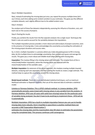
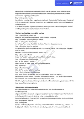
The median is more robust to outliers than the mean. However, the median alone also
doesn't provide enough informa on to judge normality.
Mode
The mode is the value that appears most frequently in a data set.
Example
Using the same data set: 2, 4, 4, 4, 5, 5, 7, 9
Mode = 4 (because 4 appears the most mes)
Normality
The mode also doesn't provide a complete picture of normality. In a perfectly normal
distribu on, the mode, median, and mean would all be the same. Mul ple modes or a large
difference between the mode and mean/median can suggest non-normality.
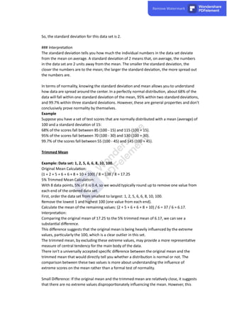
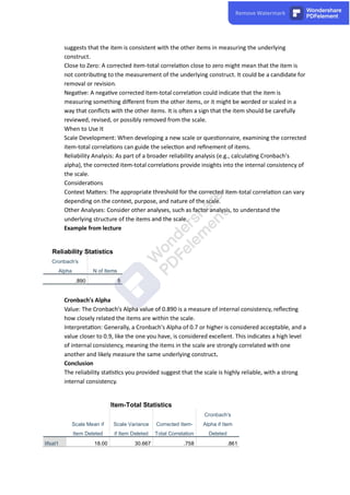
Certainly! Let's break down the calcula on of the standard devia on for the given data set
in more detail. The data set is: 2, 4, 4, 4, 5, 5, 7, 9.
### Standard Devia on
The standard devia on gives you a measure of how spread out the numbers are from the
mean. It's calculated using the following steps:
1. **Calculate the Mean**: First, you'll need to find the mean of the data.
[
text{Mean} = frac{2 + 4 + 4 + 4 + 5 + 5 + 7 + 9}{8} = 5
]
2. **Subtract the Mean and Square the Result**: Subtract the mean and square the result
for each number in the data set.
[
(2 - 5)^2 = 9
(4 - 5)^2 = 1
(4 - 5)^2 = 1
(4 - 5)^2 = 1
(5 - 5)^2 = 0
(5 - 5)^2 = 0
(7 - 5)^2 = 4
(9 - 5)^2 = 16
]
3. **Calculate the Mean of the Squared Differences**: Add up all the squared differences
and divide by the total number of numbers.
[
frac{9 + 1 + 1 + 1 + 0 + 0 + 4 + 16}{8} = frac{32}{8} = 4
]
4. **Take the Square Root**: Finally, the standard devia on is the square root of the mean
of the squared differences.
[
sqrt{4} = 2
]

So, the standard devia on for this data set is 2.
### Interpreta on
The standard devia on tells you how much the individual numbers in the data set deviate
from the mean on average. A standard devia on of 2 means that, on average, the numbers
in the data set are 2 units away from the mean. The smaller the standard devia on, the
closer the numbers are to the mean; the larger the standard devia on, the more spread out
the numbers are.
In terms of normality, knowing the standard devia on and mean allows you to understand
how data are spread around the center. In a perfectly normal distribu on, about 68% of the
data will fall within one standard devia on of the mean, 95% within two standard devia ons,
and 99.7% within three standard devia ons. However, these are general proper es and don't
conclusively prove normality by themselves.
Example
Suppose you have a set of test scores that are normally distributed with a mean (average) of
100 and a standard devia on of 15:
68% of the scores fall between 85 (100 - 15) and 115 (100 + 15).
95% of the scores fall between 70 (100 - 30) and 130 (100 + 30).
99.7% of the scores fall between 55 (100 - 45) and 145 (100 + 45).
Trimmed Mean
Example: Data set: 1, 2, 5, 6, 6, 8, 10, 100.
Original Mean Calcula on:
(1 + 2 + 5 + 6 + 6 + 8 + 10 + 100) / 8 = 138 / 8 = 17.25
5% Trimmed Mean Calcula on:
With 8 data points, 5% of 8 is 0.4, so we would typically round up to remove one value from
each end of the ordered data set.
First, order the data set from smallest to largest: 1, 2, 5, 6, 6, 8, 10, 100.
Remove the lowest 1 and highest 100 (one value from each end).
Calculate the mean of the remaining values: (2 + 5 + 6 + 6 + 8 + 10) / 6 = 37 / 6 ≈ 6.17.
Interpreta on:
Comparing the original mean of 17.25 to the 5% trimmed mean of 6.17, we can see a
substan al difference.
This difference suggests that the original mean is being heavily influenced by the extreme
values, par cularly the 100, which is a clear outlier in this set.
The trimmed mean, by excluding these extreme values, may provide a more representa ve
measure of central tendency for the main body of the data.
There isn't a universally accepted specific difference between the original mean and the
trimmed mean that would directly tell you whether a distribu on is normal or not. The
comparison between these two values is more about understanding the influence of
extreme scores on the mean rather than a formal test of normality.
Small Difference: If the original mean and the trimmed mean are rela vely close, it suggests
that there are no extreme values dispropor onately influencing the mean. However, this

doesn't necessarily mean the distribu on is normal. It could s ll be skewed or have other
features that deviate from normality.
Large Difference: If there's a significant difference between the original mean and the
trimmed mean, it indicates that there are extreme values influencing the mean. This might
point to outliers, which could suggest a non-normal distribu on, but again, it's not defini ve
on its own.
The comparison between the original and trimmed means can provide insight into the
robustness of the mean and the poten al influence of outliers, but it doesn't offer a direct
test of normality. Other tests and methods are typically used to assess normality, such as:
Graphical Methods: Histograms, Q-Q plots, and P-P plots.
Sta s cal Tests: Shapiro-Wilk, Anderson-Darling, Kolmogorov-Smirnov tests.
Skewness and Kurtosis: Examining these sta s cs can provide more insight into the shape of
the distribu on.
If normality is crucial for your analysis (e.g., if you are using parametric sta s cal methods
that assume normally distributed data), you would generally need to use these other
methods in combina on with examining the mean and other descrip ve sta s cs to assess
the normality of your data.
skewness and kurtosis
Skewness and kurtosis can be used as indicators to test for normality.
Skewness
Skewness measures the asymmetry of a probability distribu on about its mean. In a normal
distribu on, the skewness is zero.
If the skewness is less than 0, the data are spread out more to the le of the mean than to
the right.
If the skewness is greater than 0, the data are spread out more to the right.
If the skewness is close to 0, it indicates that the data are fairly symmetrical.
Kurtosis
Kurtosis measures the "tailedness" of the probability distribu on. In a normal distribu on,
the kurtosis is 3.
If the kurtosis is greater than 3, the distribu on has heavier tails and a sharper peak than the
normal distribu on.
If the kurtosis is less than 3, the distribu on has lighter tails and a fla er peak than the
normal distribu on.
If the kurtosis is close to 3, it resembles the normal distribu on in terms of tailedness.

Example
Let's consider three diﬀerent datasets:
A normal distribu on with mean 0 and standard devia on 1.
A skewed distribu on (e.g., log-normal).
A distribu on with heavy tails (e.g., t-distribu on with low degrees of freedom).
We will calculate the skewness and kurtosis for these three distribu ons and plot them to
visualize their shapes.
Normal Distribu on:
Skewness: Close to 0, indica ng symmetry.
Kurtosis: Close to 3, indica ng that the tails are similar to a normal distribu on.
The plot shows the familiar bell curve shape of the normal distribu on.

Log-Normal Distribu on:
Skewness: Greater than 0, indica ng that the data are spread out more to the right.
Kurtosis: Greater than 3, indica ng heavier tails.
The plot shows a right-skewed shape, and the peak is sharper than the normal distribu on.
If skewness is close to 0 and kurtosis is close to 3, the distribu on is likely close to normal.
However, these are just indicators, not deﬁni ve tests.
For a more formal test of normality, you might consider using sta s cal tests like the
Shapiro-Wilk test, the Anderson-Darling test, or the Kolmogorov-Smirnov test, which are
designed to test if a sample comes from a normal distribu on.
Kurtosis
Kurtosis measures the "tailedness" of a probability distribu on.
Normal Distribu on: A normal distribu on has a kurtosis of 3.
Excess Kurtosis: O en, the kurtosis value is presented as the "excess kurtosis," calculated as
the kurtosis minus 3. An excess kurtosis of 0 indicates a normal distribu on.
Leptokur c: If the kurtosis is greater than 3 (or excess kurtosis greater than 0), the
distribu on has heavier tails than the normal distribu on.
Platykur c: If the kurtosis is less than 3 (or excess kurtosis less than 0), the distribu on has
lighter tails than the normal distribu on.
Standard Error
The standard error (SE) is a measure of how much the sample mean is expected to vary from
the true popula on mean. It is calculated as:

where �n is the sample size.
Lower SE: Indicates that the sample mean is a more reliable es mator of the popula on
mean.
Higher SE: Indicates that the sample mean may deviate more from the popula on mean.
Example
Kurtosis & Excess Kurtosis: The kurtosis is close to 0, indica ng that the tails are similar to a
normal distribu on.
Standard Error: The standard error is rela vely small, sugges ng that the sample mean is a
reliable es mator of the popula on mean.

Kolmogorov-Smirnov Test
The K-S test compares the empirical distribu on func on of the sample data with the
cumula ve distribu on func on of a reference distribu on (in this case, the normal
distribu on).
Null Hypothesis: The sample comes from the specified distribu on (normal distribu on).
Alterna ve Hypothesis: The sample does not come from the specified distribu on.
Shapiro-Wilk Test
The Shapiro-Wilk test is more specific to normality and tests the null hypothesis that the data
were drawn from a normal distribu on.
Null Hypothesis: The sample comes from a normal distribu on.
Alterna ve Hypothesis: The sample does not come from a normal distribu on.
What is a p-value?
The p-value is a probability that helps us decide whether the sample data support a specific
sta s cal statement or hypothesis.
If the p-value is small (usually less than 0.05), it means that the observed data are unlikely
under the assumed hypothesis, so we reject that hypothesis.
If the p-value is large (usually greater than or equal to 0.05), it means that the observed data
are likely under the assumed hypothesis, so we don't reject it.
Example: Finding a Four-Leaf Clover
Imagine you're looking for four-leaf clovers in a field where you believe 99% of the clovers
have three leaves, and only 1% have four leaves.
Not Surprising (High P-Value): You find 99 three-leaf clovers and 1 four-leaf clover. This result
is what you'd expect, so the p-value (or "surprise score") is high.
Very Surprising (Low P-Value): You find 50 three-leaf clovers and 50 four-leaf clovers. This
result is very surprising since you expected only 1% to have four leaves, so the p-value is very
low.
 What is a α -value?
�α: The significance level, usually set before conduc ng a sta s cal test.
Value: Common choices for �α include 0.05, 0.01, or 0.10.
Purpose
Threshold for Significance: �α serves as a cut-off point for determining whether a result is
sta s cally significant.
Type I Error Rate: �α is the probability of rejec ng the null hypothesis when it is actually
true (a "false posi ve").
Usage in Hypothesis Tes ng
When conduc ng a hypothesis test, you compare the p-value (probability of observing the
data given that the null hypothesis is true) to �α:
If �≤�p≤α: The result is sta s cally significant, and you reject the null hypothesis.
If �>�p>α: The result is not sta s cally significant, and you fail to reject the null
hypothesis.
Example

Imagine you're tes ng a new medica on and want to know if it's more effec ve than an
exis ng one.
Null Hypothesis (�0H0): The new medica on is no more effec ve than the exis ng one.
Alterna ve Hypothesis (��Ha): The new medica on is more effec ve.
You choose �=0.05α=0.05, conduct the test, and get a p-value of 0.03.
Since �=0.03<�=0.05p=0.03<α=0.05, you reject the null hypothesis and conclude that the
new medica on is more effec ve.
Example simple
Analogy: Fishing Contest
Imagine you're in a fishing contest, and you want to prove that a par cular lake has
unusually large fish.
P-Value (�p): The size of the smallest fish that surprises you.
Significance Level (�α): The size of the fish that you decide will count as "large."
Example 1: Successful Fishing
Set the Standard (�α): You decide that any fish over 10 inches counts as "large"
(�=10α=10).
Catch a Fish (�p): You catch a fish that is 12 inches long (�=12p=12).
Decision for Example 1
Since the fish is larger than your standard for "large" (�>�p>α), you conclude that you have
evidence of unusually large fish in the lake.
Example 2: Unsuccessful Fishing
Set the Standard (�α): Same standard, any fish over 10 inches counts as "large"
(�=10α=10).
Catch a Fish (�p): You catch a fish that is 8 inches long (�=8p=8).
Decision for Example 2
Since the fish is smaller than your standard for "large" (�<�p<α), you conclude that you
don't have evidence of unusually large fish in the lake.
Summary in Simple Terms
P-Value (�p): The size of the fish you catch.
Significance Level (�α): The size that you decide counts as "large."
Decision: If the fish is larger than the standard (�>�p>α), you have evidence of large fish. If
the fish is smaller (�<�p<α), you don't.
The p-value and significance level in sta s cs work in a similar way. They help you decide
whether what you observe (e.g., the size of the fish) is surprising or significant based on the
standard you set.

Scenario: Project Comple on Times
Imagine you're a project manager, and you want to know if the comple on mes for a series
of projects are consistently on schedule (follow a normal distribu on) or if there are
significant varia ons (not normal).
Null Hypothesis: Project comple on mes follow a normal distribu on (on schedule).
Alterna ve Hypothesis: Project comple on mes do not follow a normal distribu on
(varia ons).
Se ng the Standard (�α)
You decide on a significance level of �=0.05α=0.05. This is like se ng a strict standard for
what you'll consider as evidence of varia on in comple on mes.
Conduc ng a Normality Test (Calcula ng �p)
You collect data on the comple on mes for 50 recent projects and apply a sta s cal test
(e.g., Shapiro-Wilk) to check for normality. The test returns a p-value, which tells you how
surprising the observed comple on mes would be if they were truly normal.
Example 1: Evidence of Normality
P-Value (�p): The test returns �=0.07p=0.07.
Comparison with �α: Since �>�p>α, the result is not significant.
Conclusion: You fail to reject the null hypothesis, meaning you don't have evidence that the
comple on mes vary from a normal distribu on. The projects are generally on schedule.
Example 2: Evidence of Non-Normality
P-Value (�p): The test returns �=0.02p=0.02.
Comparison with �α: Since �<�p<α, the result is significant.
Conclusion: You reject the null hypothesis, meaning you have evidence that the comple on
mes do not follow a normal distribu on. There might be inconsistencies in project
scheduling, and further inves ga on is needed.
Summary in Project Management Terms
P-Value (�p): A measure of how surprising the project comple on mes are if they were
supposed to be consistent (normal).
Significance Level (�α): The strictness of the standard you set for considering the
comple on mes inconsistent.
Normality: If the p-value is greater than �α, the comple on mes are consistent with
normality (on schedule). If the p-value is less than �α, they are not (inconsistent
scheduling).
This example illustrates how sta s cal concepts like the p-value and significance level can be
applied in project management to understand and control processes, such as project
comple on mes, by assessing their normality.
I hope this example helps clarify these concepts in a project management context! If you
have further ques ons or need addi onal details, please let me know.

Example from lecture
Step-by-Step Guide to Tes ng for Normality in SPSS
Open Your Data: Load or enter the dataset you want to test for normality into SPSS. This
could be a single variable like project comple on mes, customer sa sfac on scores, etc.
Choose the Test: Go to the "Analyze" menu, then select "Descrip ve Sta s cs" and choose
"Explore." This will open the Explore dialog box.
Select the Variable: In the Explore dialog box, move the variable you want to test into the
"Dependent List" box.
Choose the Normality Test: Click the "Plots" bu on, and then check the "Normality plots
with tests" box. This will usually perform the Shapiro-Wilk and Kolmogorov-Smirnov tests,
which are commonly used to test for normality.
Run the Analysis: Click "OK" to run the analysis.
View the Results: The output window will display the results, including the p-value for the
normality tests.
Descriptives
Statistic Std. Error
q1a Mean 4.32 .031
95% Confidence Interval for
Mean
Lower Bound 4.26
Upper Bound 4.38
5% Trimmed Mean 4.38
Median 4.00
Variance .511
Std. Deviation .715
Minimum 1
Maximum 5
Range 4
Interquartile Range 1
Skewness -.964 .106
Kurtosis 1.320 .211
Mean: The average value is 4.32.
Standard Error of the Mean: The standard error is 0.031, indica ng the standard devia on of
the sample mean's distribu on.
95% Conﬁdence Interval for Mean: The mean is likely to lie between 4.26 and 4.38 (with 95%
conﬁdence).
5% Trimmed Mean: This is the mean a er trimming 5% of the smallest and largest values,
and it's 4.38. It can provide a robust es mate of central tendency.

Median: The middle value is 4.00.
Variance: A measure of dispersion, it's 0.511.
Standard Devia on: The standard devia on is 0.715, providing a measure of the spread of
the distribu on.
Minimum & Maximum: The data range from 1 to 5.
Range: The difference between the maximum and minimum, 4.
Interquar le Range: The difference between the third and first quar les, 1. It's a robust
measure of spread.
Skewness: The skewness is -0.964, indica ng a le -skewed distribu on (tail on the le side).
A skewness of 0 would be expected for a perfectly normal distribu on.
Kurtosis: The kurtosis is 1.320. A kurtosis of 0 would be expected for a normal distribu on.
Posi ve kurtosis indicates a "heavier" tail and a more peaked distribu on than the normal
distribu on.
Indica on of Normality
Mean vs. Median: The mean and median are different (4.32 vs. 4.00), sugges ng a lack of
symmetry.
Skewness: The nega ve skewness indicates a distribu on that is not symmetrical, further
sugges ng non-normality.
Kurtosis: Posi ve kurtosis indicates a distribu on with tails heavier than a normal
distribu on.
Conclusion
Based on the provided descrip ve sta s cs, par cularly the skewness and kurtosis, the
distribu on of the variable q1a does not appear to follow a normal distribu on. It seems to
be le -skewed with heavier tails.
If normality is a crucial assump on for your analysis, you may want to consider
transforma ons or non-parametric methods, or explore the distribu on further using
graphical tools like histograms or Q-Q plots. Sta s cal tests like the Shapiro-Wilk or
Kolmogorov-Smirnov tests could also provide a more formal assessment of normality.
Tests of Normality
Kolmogorov-Smirnova
Shapiro-Wilk
Statistic df Sig. Statistic df Sig.
q1a .276 534 .000 .770 534 .000
a. Lilliefors Significance Correction
Sta s c: 0.276
Degrees of Freedom (df): 534
Significance (Sig.): 0.000
Shapiro-Wilk Test
Sta s c: 0.770
Interpreta on of Results

P-Value (Sig.): In both tests, the significance level (p-value) is 0.000. This is below any
common threshold for significance, such as 0.05 or 0.01.
Decision: Since the p-value is less than the chosen significance level (
�
α), we reject the null hypothesis that the data follow a normal distribu on.
Conclusion: There is strong evidence to suggest that the variable q1a does not follow a
normal distribu on. Both the Kolmogorov-Smirnov and Shapiro-Wilk tests indicate non-
normality.
Summary
The results from these tests align with the previous descrip ve sta s cs (e.g., skewness and
kurtosis) and confirm that the distribu on is not normal. In prac ce, this means that if you
are planning to use sta s cal methods that assume normality, you may need to consider
alterna ve methods that do not have this assump on or apply transforma ons to the data
to achieve normality.
Histogram:
Our case, Compare by normality as below

normally distributed dataset
indica ng a normal distribu on
Q-Q Plot (Quan le-Quan le Plot):

Q-Q Plot: Points deviate from the straight line, especially at the ends, indica ng non-normality
Compare by normality as below

Another example
Descriptives
Statistic Std. Error
Total Staff Satisfaction Scale Mean 33.97 .319
95% Confidence Interval for
Mean
Lower Bound 33.34
Upper Bound 34.60
5% Trimmed Mean 34.02
Median 34.00
Variance 49.964
Std. Deviation 7.069
Minimum 10
Maximum 50
Range 40
Interquartile Range 10
Skewness -.096 .110
Kurtosis -.147 .220
Indica on of Normality
Skewness and Kurtosis: Both skewness and kurtosis values are close to 0, which is a good
indica on of normality.
Mean vs. Median: The mean and median are almost the same (33.97 vs. 34.00), further
sugges ng symmetry.
Conclusion
Based on the provided descrip ve sta s cs, the distribu on of the "Total Staff Sa sfac on
Scale" appears to be approximately normal. The characteris cs of the distribu on, such as
mean, median, skewness, and kurtosis, align well with what would be expected from a
normal distribu on.
However, it's worth no ng that these descrip ve sta s cs alone may not provide a defini ve
conclusion about normality. To confirm normality, you might also consider visual methods
(e.g., histograms or Q-Q plots) or formal sta s cal tests (e.g., Shapiro-Wilk or Kolmogorov-
Smirnov tests).

normally distributed dataset
indica ng a normal distribu on

Points around the straight line, indica ng non-normality
No signiﬁcant skewness or outliers are visible, consistent with a normal

Tests of Normality
Kolmogorov-Smirnova Shapiro-Wilk
Total Staff Satisfaction Scale .045 491 .020 .994 491 .063
Sta s c: 0.045
Shapiro-Wilk Test
Sta s c: 0.994
Interpreta on of Results
The p-value, denoted as "Sig." in the table, represents the probability of observing the given
data if the null hypothesis of normality is true.
The p-value is 0.020, which is less than the common significance threshold of 0.05.
This result would lead you to reject the null hypothesis that the data follow a normal
distribu on.
Shapiro-Wilk Test
The p-value is 0.063, which is greater than the common significance threshold of 0.05.
This result would lead you to fail to reject the null hypothesis that the data follow a normal
distribu on.
Conclusion
The results of the two tests are somewhat conflic ng:
The Kolmogorov-Smirnov test indicates a significant devia on from normality (p = 0.020).
The Shapiro-Wilk test does not indicate a significant devia on from normality (p = 0.063).
In this specific case, the evidence leans slightly more towards normality, especially
considering the Shapiro-Wilk test and the previously analyzed descrip ve sta s cs.
Manipulate the data ‫البیانات‬ ‫معالجة‬
Transforming the Data: If the normality assump on is crucial for your analysis, you might
consider applying a transforma on (e.g., log, square root) to make the distribu on more
normal.
Outlier Analysis: Iden fying and handling outliers might be another considera on.
Depending on the context and the nature of the outliers, you might decide to remove, cap,
or transform them.
Subse ng or Filtering: You might want to analyze a specific subset of the data or apply some
filters based on certain criteria.

Sta s cal Analysis: Depending on your research ques on or business need, you might be
planning to conduct a speciﬁc sta s cal analysis (e.g., regression, t-test, ANOVA) using the
data.
Visualiza ons: Crea ng visualiza ons like histograms, sca er plots, or box plots can provide
valuable insights into the data's distribu on and rela onships between variables.
Handling Missing Data: If there are missing values in your data, you might need to decide
how to handle them, whether by impu ng missing values or removing incomplete cases.
Calcula on total score
Step 1: Understand the Context
Determine why there are nega ve scores in the dataset and what they represent. Are they
errors, or do they have a legi mate meaning in the context of your analysis?
Step 2: Prepare the Data
Make sure the data is clean and correctly forma ed. Handle any missing or erroneous values,
as they can aﬀect the total score calcula on.
Step 3: Decide on the Approach
Determine how you want to handle the nega ve values. Common approaches include:
Reversing: If the nega ve values represent reversed scales (e.g., in a survey where some
ques ons are worded nega vely), you might need to reverse or re-scale them.
Transforming: You might apply a transforma on to shi all values into a posi ve range.
Removing: If nega ve values represent errors or invalid data, you might choose to remove or
replace them.

TestsofNormality
Kolmogorov-Smirnova
Shapiro-Wilk
TotalStaffSatisfactionScale .045 491 .020 .994 491 .063
Kolmogorov-SmirnovTest
Sta s c:0.045
DegreesofFreedom(df):491
Significance(Sig.):0.020
Shapiro-WilkTest
Sta s c:0.994
DegreesofFreedom(df):491
Significance(Sig.):0.063
Interpreta onofResults
Thep-
value,denotedas"Sig."inthetable,representstheprobabilityofobservingthegivendatai henullh
ypothesisofnormalityistrue.
Kolmogorov-SmirnovTest
Thep-valueis0.020,whichislessthanthecommonsignificancethresholdof0.05.
Thisresultwouldleadyoutorejec henullhypothesistha hedatafollowanormaldistribu on.
Shapiro-WilkTest
Thep-valueis0.063,whichisgreaterthanthecommonsignificancethresholdof0.05.
Thisresultwouldleadyoutofailtorejec henullhypothesistha hedatafollowanormaldistribu on
.
Conclusion
Theresultso hetwotestsaresomewhatconflic ng:
TheKolmogorov-Smirnovtes ndicatesasignificantdevia onfromnormality(p=0.020).
TheShapiro-Wilktestdoesno ndicateasignificantdevia onfromnormality(p=0.063).
Inthisspecificcase,theevidenceleansslightlymoretowardsnormality,especiallyconsideringthe
Shapiro-Wilktestandthepreviouslyanalyzeddescrip vesta s cs.
TransformingtheData:I henormalityassump oniscrucialforyouranalysis,youmightconsiderap
plyingatransforma on(e.g.,log,squareroot)tomakethedistribu onmorenormal.
OutlierAnalysis:Iden fyingandhandlingoutliersmightbeanotherconsidera on.Dependingonth
econtextandthenatureo heoutliers,youmightdecidetoremove,cap,ortransformthem.
Subse ngorFiltering:Youmightwan oanalyzeaspecificsubseto hedataorapplysomefiltersbas
edoncertaincriteria.

Sta s calAnalysis:Dependingonyourresearchques onorbusinessneed,youmightbeplanningt
oconductaspecificsta s calanalysis(e.g.,regression,t-test,ANOVA)usingthedata.
Visualiza ons:Crea ngvisualiza onslikehistograms,sca erplots,orboxplotscanprovidevaluabl
einsightsintothedata'sdistribu onandrela onshipsbetweenvariables.
HandlingMissingData:I herearemissingvaluesinyourdata,youmightneedtodecidehowtohandl
ethem,whetherbyimpu ngmissingvaluesorremovingincompletecases.
Preparing Data:
Collect Data: Gather all survey responses.
Iden fy Nega ve Items: Mark any nega vely worded items that need to be reversed.
Clean and Format Data: Structure the data appropriately, ready for SPSS.
Adding Data to SPSS:
Import File: Open SPSS and import the data file.
Define Variables: Set variable a ributes like types, labels, and measurement levels.
Reversing Nega ve Worded Items:
Select Nega ve Items: Iden fy the variables represen ng nega vely worded ques ons.
Reverse Scores: Use the "Compute" op on to reverse the scores (e.g., if using a 5-point scale,
you could use the expression 5 - variable_name).
Calcula ng Total Scores:
Select Variables: Iden fy the variables you want to sum, including reversed ones.
Compute Total Score: Create a new variable that sums the selected variables.
Review Results: Ensure accuracy in the computed total scores.
Another method
Transform------recode in to same or different variables and change the scale to be 1—5 and 2
---4 ,…etc for 5 scale
step-by-step guide to doing that total score step by spss:
Step 1: Open SPSS Data File
Open the SPSS data file where you have the variables you want to sum.
Step 2: Iden fy the Variables to Sum
Determine which variables you want to include in the total score. These might be individual
survey items, test scores, etc.
Step 3: Use the Compute Variable Func on
Click on "Transform" in the menu bar.
Select "Compute Variable" from the drop-down menu.
Step 4: Create the Total Score Variable
In the "Compute Variable" dialog box, type a name for the new variable in the "Target
Variable" field (e.g., total_score).
In the "Numeric Expression" field, enter an expression to sum the variables. For example, if
you want to sum variables item1, item2, and item3, you would enter item1 + item2 + item3.
Click "OK" to compute the new variable.
Step 5: Validate the Total Score

Check the newly computed variable in the Data View to ensure that the total score has been
calculated correctly.
Consider running descrip ve sta s cs to understand the distribu on of the total score.
Step 6: Save the Changes
Save the SPSS data file to keep the changes.
collapsing variable in to group
Step 1: Open Your SPSS Data File
Open the SPSS data file containing the variable you want to collapse.
Step 2: Iden fy the Variable to Collapse
Determine the variable you wish to collapse into groups and the criteria for grouping.
Step 3: Use the Recode Func on
Click on "Transform" in the menu bar.
Select "Recode into Different Variables..." from the drop-down menu.
Step 4: Set Up the Recode
Select the variable you want to collapse from the list of available variables.
Type a name for the new variable in the "Output Variable" sec on.
Click on "Change."
Step 5: Define the Groups
Click on "Old and New Values."
Enter the original values (or range of values) and the new values to define the groups.
For example, you can collapse a variable with values 1 to 10 into three groups: 1-3, 4-7, and
8-10.
Click on "Add" a er defining each group.
Click on "Con nue" when done.
Step 6: Execute the Recode
Click on "OK" in the Recode into Different Variables dialog box to execute the recode.
Step 7: Validate the New Variable
Check the newly created variable in the Data View to ensure that the recode has been
performed correctly.
Consider running frequencies or other descrip ve sta s cs to understand the distribu on of
the new groups.
Step 8: Save the Changes
Save the SPSS data file to keep the changes.
Checking the reliability of a scale
how to check the reliability for a scale in SPSS:
Open the SPSS data file containing the variables (items) that make up the scale you want to
assess.
Step 2: Select the Reliability Analysis Op on
Click on "Analyze" in the menu bar.

Go to "Scale" and select "Reliability Analysis..." from the drop-down menu.
Step 3: Select the Items for the Scale
In the Reliability Analysis dialog box, select the variables (items) that make up the scale you
want to assess.
Move the selected variables into the "Items" box.
Step 4: Choose the Reliability Coefficient
Click on the "Sta s cs" bu on.
Select "Scale if item deleted" to see how the reliability coefficient changes if each item is
removed from the scale.
Click "Con nue."
Step 5: Choose the Model
Under the "Model" sec on, select "Alpha" for Cronbach's alpha, which is a standard measure
of internal consistency.
Op onally, you can explore other models, but Cronbach's alpha is commonly used for scale
reliability.
Step 6: Run the Analysis
Click "OK" to run the reliability analysis.
Step 7: Interpret the Results
Review the Output window for the results.
Look for the "Cronbach's Alpha" value, which will range from 0 to 1. A common rule of
thumb is that an alpha of 0.7 or higher indicates acceptable reliability, although this can vary
depending on the context and purpose of the scale.
An inter-item correla on matrix
Here's how to generate an inter-item correla on matrix in SPSS, including looking for
nega ve values:
Open the SPSS data file containing the items you want to analyze.
Step 2: Select the Correla on Analysis Op on
Go to "Correlate" and select "Bivariate..." from the drop-down menu.
Step 3: Select the Items to Include
In the Bivariate Correla ons dialog box, select the variables (items) you want to include in
the correla on matrix.
Move the selected variables into the "Variables" box.
Step 4: Choose the Correla on Coefficient
Select the correla on coefficient you want to use (e.g., Pearson).
If you want to include significance levels, make sure the "Flag significant correla ons" box is
checked.
Click "OK" to run the correla on analysis.
Step 6: Review the Correla on Matrix
Look at the Output window to view the correla on matrix.

Examine the correla ons between items, paying special a en on to any nega ve values.
Nega ve correla ons may indicate that two items are inversely related, which could be
expected for nega vely worded items.
Step 7: Interpret the Results
Consider the meaning of any nega ve correla ons in the context of the items and the overall
scale or ques onnaire. Nega ve correla ons with nega vely worded items may be expected
and appropriate.
If you find unexpected nega ve correla ons, this may warrant further inves ga on into the
wording, scaling, or conceptual alignment of the items.
The item-total sta s cs in reliability analysis
Open the SPSS data file containing the items you want to analyze.
Step 2: Select the Reliability Analysis Op on
Go to "Scale" and select "Reliability Analysis..." from the drop-down menu.
Step 3: Select the Items for Analysis
In the Reliability Analysis dialog box, select the variables (items) that make up the scale you
want to assess.
Move the selected variables into the "Items" box.
Step 4: Choose the Model
Under the "Model" sec on, select "Alpha" for Cronbach's alpha.
Step 5: Request Item-Total Sta s cs
Click on the "Sta s cs" bu on.
Check the box for "Item, scale, and scale if item deleted."
Click "Con nue."
Click "OK" to run the reliability analysis.
Step 7: Review the Item-Total Sta s cs
Look at the Output window and find the table labeled "Item-Total Sta s cs."
Examine the column labeled "Corrected Item-Total Correla on." This shows the correla on
between each item and the total score of the remaining items.
Iden fy any items with a correla on greater than 0.3. These items strongly correlate with the
total score of the remaining items.
The corrected item-total correla on
the corrected item-total correla on is important and how you can interpret it:
What It Represents
Alignment with the Construct: A high corrected item-total correla on means that the item is
well-aligned with the overall construct being measured by the scale.
Poten al Redundancy: Extremely high correla ons might suggest that the item is redundant
with other items in the scale.
How to Interpret It
Posi ve and Strong: A posi ve and strong corrected item-total correla on (e.g., above 0.3 or
0.4) typically indicates that the item is contribu ng posi vely to the scale's reliability. It

suggests that the item is consistent with the other items in measuring the underlying
construct.
Close to Zero: A corrected item-total correla on close to zero might mean that the item is
not contribu ng to the measurement of the underlying construct. It could be a candidate for
removal or revision.
Nega ve: A nega ve corrected item-total correla on could indicate that the item is
measuring something different from the other items, or it might be worded or scaled in a
way that conflicts with the other items. It is o en a sign that the item should be carefully
reviewed, revised, or possibly removed from the scale.
When to Use It
Scale Development: When developing a new scale or ques onnaire, examining the corrected
item-total correla ons can guide the selec on and refinement of items.
Reliability Analysis: As part of a broader reliability analysis (e.g., calcula ng Cronbach's
alpha), the corrected item-total correla ons provide insights into the internal consistency of
the scale.
Considera ons
Context Ma ers: The appropriate threshold for the corrected item-total correla on can vary
depending on the context, purpose, and nature of the scale.
Other Analyses: Consider other analyses, such as factor analysis, to understand the
underlying structure of the items and the scale.
Example from lecture
Reliability Statistics
Cronbach's
Alpha N of Items
.890 5
Cronbach's Alpha
Value: The Cronbach's Alpha value of 0.890 is a measure of internal consistency, reflec ng
how closely related the items are within the scale.
Interpreta on: Generally, a Cronbach's Alpha of 0.7 or higher is considered acceptable, and a
value closer to 0.9, like the one you have, is considered excellent. This indicates a high level
of internal consistency, meaning the items in the scale are strongly correlated with one
another and likely measure the same underlying construct.
Conclusion
The reliability sta s cs you provided suggest that the scale is highly reliable, with a strong
internal consistency.
Item-Total Statistics
Scale Mean if
Item Deleted
Scale Variance
if Item Deleted
Corrected Item-
Total Correlation
Cronbach's
Alpha if Item
Deleted
lifsat1 18.00 30.667 .758 .861

lifsat2 17.81 30.496 .752 .862
lifsat3 17.69 29.852 .824 .847
lifsat4 17.63 29.954 .734 .866
lifsat5 18.39 29.704 .627 .896
Corrected Item-Total Correla on
This is the correla on between each item and the total score of the remaining items. It's a
key indicator of how well each item aligns with the overall construct:
All the correla ons are posi ve and rela vely strong (ranging from 0.627 to 0.824),
sugges ng that all items are well-aligned with the overall construct.
lifsat3 has the highest correla on (0.824), meaning it is most strongly associated with the
total score of the other items.
lifsat5 has the lowest correla on (0.627), but it is s ll above the commonly accepted
threshold of 0.3, indica ng a good alignment.
Cronbach's Alpha if Item Deleted
This shows the overall Cronbach's Alpha for the scale if a par cular item is deleted:
The original Cronbach's Alpha for the scale is 0.890.
If any item is deleted, the Cronbach's Alpha remains within a similar range (from 0.847 to
0.896), sugges ng that no single item is drama cally aﬀec ng the overall reliability.
Dele ng lifsat5 would result in the highest Cronbach's Alpha (0.896), but the diﬀerences are
minimal, so there might not be a compelling reason to remove any item.
Conclusion
The sta s cs indicate a well-constructed and reliable scale, where each item contributes
posi vely to the overall construct being measured. There's no apparent evidence from these
sta s cs to suggest that any item should be removed or revised. Of course, these
quan ta ve insights should be considered alongside qualita ve understanding of the scale's
content, purpose, and context.

SPSS GuideAssessing Normality, Handling Missing Data, and Calculating Scores.pdf

Recommended

Recommended

More Related Content

Similar to SPSS GuideAssessing Normality, Handling Missing Data, and Calculating Scores.pdf

Similar to SPSS GuideAssessing Normality, Handling Missing Data, and Calculating Scores.pdf (20)

Recently uploaded

Recently uploaded (20)

SPSS GuideAssessing Normality, Handling Missing Data, and Calculating Scores.pdf