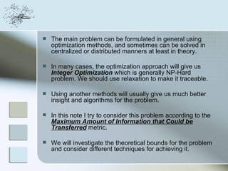
Download to read offline


![Re ed − Solomon R ( n, k ) ::
→
M 1×k = [ M 0 , M 1 ,..., M k −1 ]
{α1 , α2 ,..., αn } ∈ GF (q) , ∀αi ≠ 0.
→
C1×n = [C0 , C1 ,..., Cn −1 ]
1 1 ... 1
→ →
α1 α2 ... α n
C 1×n = M 1×k
. . ... .
k −1
α 1 α k −12 k −1
... α n
The structure of the above matrix is Vandermonde
And with any h subset of the Codeword we can make
the original message.](https://image.slidesharecdn.com/networkinformationprocessing-120615145703-phpapp02/85/Network-Information-Processing-52-320.jpg)


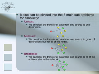
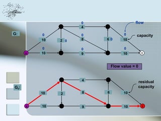
This document discusses network information processing and maximum information transfer in networks. It begins by formulating the main problems of unicast, multicast, and broadcast transfer of data in a network. It then shows that the maximum information transfer for unicast can be determined using the maximum flow minimum cut theorem, which gives a polynomial time solution. For multicast, maximum transfer is bounded by considering a super terminal node, but achieving maximum diversity at destinations is challenging. The document explores duplicate-and-forward routing and network coding approaches for multicast transfer.