AACIMP 2010 Summer School lecture by Leonidas Sakalauskas. "Applied Mathematics" stream. "Stochastic Programming and Applications" course. Part 5.
More info at http://summerschool.ssa.org.ua
International Conference on Monte Carlo techniques
Closing conference of thematic cycle
Paris July 5-8th 2016
Campus les cordeliers
Chris Sherlock's slides
Sequential quasi-Monte Carlo (SQMC) is a quasi-Monte Carlo (QMC) version of sequential Monte Carlo (or particle filtering), a popular class of Monte Carlo techniques used to carry out inference in state space models. In this talk I will first review the SQMC methodology as well as some theoretical results. Although SQMC converges faster than the usual Monte Carlo error rate its performance deteriorates quickly as the dimension of the hidden variable increases. However, I will show with an example that SQMC may perform well for some "high" dimensional problems. I will conclude this talk with some open problems and potential applications of SQMC in complicated settings.
In this talk we consider the question of how to use QMC with an empirical dataset, such as a set of points generated by MCMC. Using ideas from partitioning for parallel computing, we apply recursive bisection to reorder the points, and then interleave the bits of the QMC coordinates to select the appropriate point from the dataset. Numerical tests show that in the case of known distributions this is almost as effective as applying QMC directly to the original distribution. The same recursive bisection can also be used to thin the dataset, by recursively bisecting down to many small subsets of points, and then randomly selecting one point from each subset. This makes it possible to reduce the size of the dataset greatly without significantly increasing the overall error. Co-author: Fei Xie
International Conference on Monte Carlo techniques
Closing conference of thematic cycle
Paris July 5-8th 2016
Campus les cordeliers
Jere Koskela's slides
Nonlinear Stochastic Programming by the Monte-Carlo methodSSA KPI
AACIMP 2010 Summer School lecture by Leonidas Sakalauskas. "Applied Mathematics" stream. "Stochastic Programming and Applications" course. Part 4.
More info at http://summerschool.ssa.org.ua
In this talk, we discuss some recent advances in probabilistic schemes for high-dimensional PIDEs. It is known that traditional PDE solvers, e.g., finite element, finite difference methods, do not scale well with the increase of dimension. The idea of probabilistic schemes is to link a wide class of nonlinear parabolic PIDEs to stochastic Levy processes based on nonlinear version of the Feynman-Kac theory. As such, the solution of the PIDE can be represented by a conditional expectation (i.e., a high-dimensional integral) with respect to a stochastic dynamical system driven by Levy processes. In other words, we can solve the PIDEs by performing high-dimensional numerical integration. A variety of quadrature methods could be applied, including MC, QMC, sparse grids, etc. The probabilistic schemes have been used in many application problems, e.g., particle transport in plasmas (e.g., Vlasov-Fokker-Planck equations), nonlinear filtering (e.g., Zakai equations), and option pricing, etc.
We present recent result on the numerical analysis of Quasi Monte-Carlo quadrature methods, applied to forward and inverse uncertainty quantification for elliptic and parabolic PDEs. Particular attention will be placed on Higher
-Order QMC, the stable and efficient generation of
interlaced polynomial lattice rules, and the numerical analysis of multilevel QMC Finite Element discretizations with applications to computational uncertainty quantification.
Probabilistic Control of Switched Linear Systems with Chance ConstraintsLeo Asselborn
An approach to algorithmically synthesize control
strategies for set-to-set transitions of uncertain discrete-time
switched linear systems based on a combination of tree search
and reachable set computations in a stochastic setting is
proposed in this presentation. The initial state and disturbances
are assumed to be Gaussian distributed, and a time-variant
hybrid control law stabilizes the system towards a goal set.
The algorithmic solution computes sequences of discrete states
via tree search and the continuous controls are obtained
from solving embedded semi-definite programs (SDP). These
program taking polytopic input constraints as well as timevarying
probabilistic state constraints into account. An example
for demonstrating the principles of the solution procedure with
focus on handling the chance constraints is included.
Basic Computer Engineering Unit II as per RGPV SyllabusNANDINI SHARMA
Algorithm, Flowchart, Categories of Programming Languages, OOPs vs POP, concepts of OOPs, Inheritance, C++ Programming, How to write C++ program as a beginner, Array, Structure, etc
Unit 1: Fundamentals of the Analysis of Algorithmic Efficiency, Units for Measuring Running Time, PROPERTIES OF AN ALGORITHM, Growth of Functions, Algorithm - Analysis, Asymptotic Notations, Recurrence Relation and problems
TIME EXECUTION OF DIFFERENT SORTED ALGORITHMSTanya Makkar
what is Algorithm and classification and its complexity
Time Complexity
Time Space trade-off
Asymptotic time complexity of algorithm and its notation
Why do we need to classify running time of algorithm into growth rates?
Big O-h notation and example
Big omega notation and example
Big theta notation and its example
best among the 3 notation
finding complexity f(n) for certain cases
1. Average case
2.Best case
3.Worst case
Searching
Sorting
complexity of Sorting
Conclusion
Let's dive deeper into the world of ODC! Ricardo Alves (OutSystems) will join us to tell all about the new Data Fabric. After that, Sezen de Bruijn (OutSystems) will get into the details on how to best design a sturdy architecture within ODC.
"Impact of front-end architecture on development cost", Viktor TurskyiFwdays
I have heard many times that architecture is not important for the front-end. Also, many times I have seen how developers implement features on the front-end just following the standard rules for a framework and think that this is enough to successfully launch the project, and then the project fails. How to prevent this and what approach to choose? I have launched dozens of complex projects and during the talk we will analyze which approaches have worked for me and which have not.
Slack (or Teams) Automation for Bonterra Impact Management (fka Social Soluti...Jeffrey Haguewood
Sidekick Solutions uses Bonterra Impact Management (fka Social Solutions Apricot) and automation solutions to integrate data for business workflows.
We believe integration and automation are essential to user experience and the promise of efficient work through technology. Automation is the critical ingredient to realizing that full vision. We develop integration products and services for Bonterra Case Management software to support the deployment of automations for a variety of use cases.
This video focuses on the notifications, alerts, and approval requests using Slack for Bonterra Impact Management. The solutions covered in this webinar can also be deployed for Microsoft Teams.
Interested in deploying notification automations for Bonterra Impact Management? Contact us at sales@sidekicksolutionsllc.com to discuss next steps.
Accelerate your Kubernetes clusters with Varnish CachingThijs Feryn
A presentation about the usage and availability of Varnish on Kubernetes. This talk explores the capabilities of Varnish caching and shows how to use the Varnish Helm chart to deploy it to Kubernetes.
This presentation was delivered at K8SUG Singapore. See https://feryn.eu/presentations/accelerate-your-kubernetes-clusters-with-varnish-caching-k8sug-singapore-28-2024 for more details.
Smart TV Buyer Insights Survey 2024 by 91mobiles.pdf91mobiles
91mobiles recently conducted a Smart TV Buyer Insights Survey in which we asked over 3,000 respondents about the TV they own, aspects they look at on a new TV, and their TV buying preferences.
Dev Dives: Train smarter, not harder – active learning and UiPath LLMs for do...UiPathCommunity
💥 Speed, accuracy, and scaling – discover the superpowers of GenAI in action with UiPath Document Understanding and Communications Mining™:
See how to accelerate model training and optimize model performance with active learning
Learn about the latest enhancements to out-of-the-box document processing – with little to no training required
Get an exclusive demo of the new family of UiPath LLMs – GenAI models specialized for processing different types of documents and messages
This is a hands-on session specifically designed for automation developers and AI enthusiasts seeking to enhance their knowledge in leveraging the latest intelligent document processing capabilities offered by UiPath.
Speakers:
👨🏫 Andras Palfi, Senior Product Manager, UiPath
👩🏫 Lenka Dulovicova, Product Program Manager, UiPath
Software Delivery At the Speed of AI: Inflectra Invests In AI-Powered QualityInflectra
In this insightful webinar, Inflectra explores how artificial intelligence (AI) is transforming software development and testing. Discover how AI-powered tools are revolutionizing every stage of the software development lifecycle (SDLC), from design and prototyping to testing, deployment, and monitoring.
Learn about:
• The Future of Testing: How AI is shifting testing towards verification, analysis, and higher-level skills, while reducing repetitive tasks.
• Test Automation: How AI-powered test case generation, optimization, and self-healing tests are making testing more efficient and effective.
• Visual Testing: Explore the emerging capabilities of AI in visual testing and how it's set to revolutionize UI verification.
• Inflectra's AI Solutions: See demonstrations of Inflectra's cutting-edge AI tools like the ChatGPT plugin and Azure Open AI platform, designed to streamline your testing process.
Whether you're a developer, tester, or QA professional, this webinar will give you valuable insights into how AI is shaping the future of software delivery.
Epistemic Interaction - tuning interfaces to provide information for AI supportAlan Dix
Paper presented at SYNERGY workshop at AVI 2024, Genoa, Italy. 3rd June 2024
https://alandix.com/academic/papers/synergy2024-epistemic/
As machine learning integrates deeper into human-computer interactions, the concept of epistemic interaction emerges, aiming to refine these interactions to enhance system adaptability. This approach encourages minor, intentional adjustments in user behaviour to enrich the data available for system learning. This paper introduces epistemic interaction within the context of human-system communication, illustrating how deliberate interaction design can improve system understanding and adaptation. Through concrete examples, we demonstrate the potential of epistemic interaction to significantly advance human-computer interaction by leveraging intuitive human communication strategies to inform system design and functionality, offering a novel pathway for enriching user-system engagements.
Search and Society: Reimagining Information Access for Radical FuturesBhaskar Mitra
The field of Information retrieval (IR) is currently undergoing a transformative shift, at least partly due to the emerging applications of generative AI to information access. In this talk, we will deliberate on the sociotechnical implications of generative AI for information access. We will argue that there is both a critical necessity and an exciting opportunity for the IR community to re-center our research agendas on societal needs while dismantling the artificial separation between the work on fairness, accountability, transparency, and ethics in IR and the rest of IR research. Instead of adopting a reactionary strategy of trying to mitigate potential social harms from emerging technologies, the community should aim to proactively set the research agenda for the kinds of systems we should build inspired by diverse explicitly stated sociotechnical imaginaries. The sociotechnical imaginaries that underpin the design and development of information access technologies needs to be explicitly articulated, and we need to develop theories of change in context of these diverse perspectives. Our guiding future imaginaries must be informed by other academic fields, such as democratic theory and critical theory, and should be co-developed with social science scholars, legal scholars, civil rights and social justice activists, and artists, among others.
JMeter webinar - integration with InfluxDB and GrafanaRTTS
Watch this recorded webinar about real-time monitoring of application performance. See how to integrate Apache JMeter, the open-source leader in performance testing, with InfluxDB, the open-source time-series database, and Grafana, the open-source analytics and visualization application.
In this webinar, we will review the benefits of leveraging InfluxDB and Grafana when executing load tests and demonstrate how these tools are used to visualize performance metrics.
Length: 30 minutes
Session Overview
-------------------------------------------
During this webinar, we will cover the following topics while demonstrating the integrations of JMeter, InfluxDB and Grafana:
- What out-of-the-box solutions are available for real-time monitoring JMeter tests?
- What are the benefits of integrating InfluxDB and Grafana into the load testing stack?
- Which features are provided by Grafana?
- Demonstration of InfluxDB and Grafana using a practice web application
To view the webinar recording, go to:
https://www.rttsweb.com/jmeter-integration-webinar
Builder.ai Founder Sachin Dev Duggal's Strategic Approach to Create an Innova...Ramesh Iyer
In today's fast-changing business world, Companies that adapt and embrace new ideas often need help to keep up with the competition. However, fostering a culture of innovation takes much work. It takes vision, leadership and willingness to take risks in the right proportion. Sachin Dev Duggal, co-founder of Builder.ai, has perfected the art of this balance, creating a company culture where creativity and growth are nurtured at each stage.
State of ICS and IoT Cyber Threat Landscape Report 2024 previewPrayukth K V
The IoT and OT threat landscape report has been prepared by the Threat Research Team at Sectrio using data from Sectrio, cyber threat intelligence farming facilities spread across over 85 cities around the world. In addition, Sectrio also runs AI-based advanced threat and payload engagement facilities that serve as sinks to attract and engage sophisticated threat actors, and newer malware including new variants and latent threats that are at an earlier stage of development.
The latest edition of the OT/ICS and IoT security Threat Landscape Report 2024 also covers:
State of global ICS asset and network exposure
Sectoral targets and attacks as well as the cost of ransom
Global APT activity, AI usage, actor and tactic profiles, and implications
Rise in volumes of AI-powered cyberattacks
Major cyber events in 2024
Malware and malicious payload trends
Cyberattack types and targets
Vulnerability exploit attempts on CVEs
Attacks on counties – USA
Expansion of bot farms – how, where, and why
In-depth analysis of the cyber threat landscape across North America, South America, Europe, APAC, and the Middle East
Why are attacks on smart factories rising?
Cyber risk predictions
Axis of attacks – Europe
Systemic attacks in the Middle East
Download the full report from here:
https://sectrio.com/resources/ot-threat-landscape-reports/sectrio-releases-ot-ics-and-iot-security-threat-landscape-report-2024/
Key Trends Shaping the Future of Infrastructure.pdfCheryl Hung
Keynote at DIGIT West Expo, Glasgow on 29 May 2024.
Cheryl Hung, ochery.com
Sr Director, Infrastructure Ecosystem, Arm.
The key trends across hardware, cloud and open-source; exploring how these areas are likely to mature and develop over the short and long-term, and then considering how organisations can position themselves to adapt and thrive.
Key Trends Shaping the Future of Infrastructure.pdf
Sienna 2 analysis
1. Computer Science 385
Analysis of Algorithms
Siena College
Spring 2011
Topic Notes: Analysis Fundamentals
We will next review and expand upon some of what you know from some of your previous courses
about measuring efficiency.
Asymptotic Analysis
We want to focus on how Computer Scientists think about the differences among the costs of
various operations.
There are many ways that we can think about the “cost” of a particular computation. The most
important of which are
• computational cost: how many “basic operations” of some kind does it take to accomplish
what we are trying to do?
– If we are copying the elements of one array to another, we might count the number of
elements we need to copy.
– In other examples, we may wish to count the number of times a key operation, such as
a multiplication statement, takes place.
– We can estimate running time for a problem of size n, T (n), by multiplying the execu-
tion time of our basic operation, cop , by the number of basic operations, C(n):
T (n) ≈ cop C(n)
• space cost: how much memory do we need to use?
– may be the number of bytes, words, or some unit of data stored in a structure
The operations we’ll want to count tend to be those that happen inside of loops, or more signifi-
cantly, inside of nested loops.
Determining an exact count of operations might be useful in some circumstances, but we usually
want to look at the trends of the operation costs as we deal with larger and larger problems sizes.
This allows us to compare algorithms or structures in a general but very meaningful way without
looking at the relatively insignificant details of an implementation or worrying about characteristics
of the machine we wish to run on.
To do this, we ignore differences in the counts which are constant and look at an overall trend as
the size of the problem is increased.
2. CS 385 Analysis of Algorithms Spring 2011
n
For example, we’ll treat n and 2
as being essentially the same.
1
Similarly, 1000
n2 , 2n2 and 1000n2 are all “pretty much” n2 .
With more complex expressions, we also say that only the most significant term (the one with the
largest exponent) is important when we have different parts of the computation taking different
amounts of work or space. So if an algorithm uses n + n2 operations, as n gets large, the n2 term
dominates and we ignore the n.
In general if we have a polynomial of the form a0 nk + a1 nk−1 + ... + ak , say it is “pretty much”
nk . We only consider the most significant term.
We formalize this idea of “pretty much” using asymptotic analysis:
Definition: A function f (n) ∈ O(g(n)) if and only if there exist two positive constants c and n0
such that |f (n)| ≤ c · g(n) for all n > n0 .
Equivalently, we can say that f (n) ∈ O(g(n)) if there is a constant c such that for all sufficiently
large n, | f (n) | ≤ c.
g(n)
To satisfy these definitions, we can always choose a really huge g(n), perhaps nn , but as a rule,
n
we want a g(n) without any constant factor, and as “small” of a function as we can.
So if both g(n) = n and g(n) = n2 are valid choices, we choose g(n) = n. We can think of
g(n) as an upper bound (within a constant factor) in the long-term behavior of f (n), and in this
example, n is a “tighter bound” than n2 .
We also don’t care how big the constant is and how big n0 has to be. Well, at least not when
determining the complexity. We would care about those in specific cases when it comes to imple-
mentation or choosing among existing implementations, where we may know that n is not going
to be very large in practice, or when c has to be huge. But for our theoretical analysis, we don’t
care. We’re interested in relative rates of growth of functions.
Common Orders of Growth
The most common “orders of growth” or “orders of complexity” are
• O(1) – for any constant-time operations, such as the assignment of an element in an array.
The cost doesn’t depend on the size of the array or the position we’re setting.
• O(log n) – logarithmic factors tend to come into play in “divide and conquer” algorithms.
Example: binary search in an ordered array of n elements.
• O(n) – linear dependence on the size. This is very common, and examples include the
insertion of a new element at the beginning of an array containing n elements.
• O(n log n) – this is just a little bigger than O(n), but definitely bigger. The most famous
examples are divide and conquer sorting algorithms, which we will look at soon.
• O(n2 ) – quadratic. Most naive sorting algorithms are O(n2 ). Doubly-nested loops often
lead to this behavior. Example: matrix-matrix addition for n × n matrices.
2
3. CS 385 Analysis of Algorithms Spring 2011
• O(n3 ) – cubic complexity. Triply nested loops will lead to this behavior. A good example
is matrix-matrix multiplication. We need to do n operations (a dot product) on each of n2
matrix entries.
• O(nk ), for constant k – polynomial complexity. As k grows, the cost of these kinds of
algorithms grows very quickly.
Computer Scientists are actually very excited to find polynomial time algorithms for seem-
ingly very difficult problems. In fact, there is a whole class of problems (NP) for which if
you could either come up with a polynomial time algorithm, no matter how big k is (as long
as it’s constant), or if you could prove that no such algorithm exists, you would instantly be
world famous! At least among us Computer Scientists. We will likely introduce the idea of
NP and NP-Completeness later this semester and you will encounter this in Discrete II.
• O(2n ) – exponential complexity. Recursive solutions where we are searching for some “best
possible” solution often leads to an exponential algorithm. Constructing a “power set” from
a set of n elements requires O(2n ) work. Checking topological equivalence of circuits is one
example of a problem with exponential complexity.
• O(n!) – pretty huge
• O(nn ) – even more huge
Suppose we have operations with time complexity O(log n), O(n), O(n log n), O(n2 ), and O(2n ).
And suppose the time to solve a problem of size n is t. How much time to do problem 10, 100, or
1000 times larger?
Time to Solve Problem
size n 10n 100n 1000n
O(1) t t t t
O(log n) t > 3t ∼ 6.5t < 10t
O(n) t 10t 100t 1, 000t
O(n log n) t > 30t ∼ 650t < 10, 000t
O(n2 ) t 100t 10, 000t 1, 000, 000t
O(2n ) t ∼ t10 ∼ t100 ∼ t1000
Note that the last line depends on the fact that the constant is 1, otherwise the times are somewhat
different.
See Example:
˜jteresco/shared/cs385/examples/EfficiencyClasses/RunTimes.java
Now let’s think about complexity from a different perspective.
Suppose we get a faster computer, 10, 100, or 1000 times faster than the one we had, or we’re
willing to wait 10, 100, or 1000 times longer to get our solution if we can solve a larger problem.
How much larger problems can be solved? If original machine allowed solution of problem of size
k in time t, then how big a problem can be solved in some multiple of t?
3
4. CS 385 Analysis of Algorithms Spring 2011
Problem Size
speed-up 1x 10x 100x 1000x
10
O(log n) k k k 100 k 1000
O(n) k 10k 100k 1, 000k
O(n log n) k < 10k < 100k < 1, 000k
O(n2 ) k 3k+ 10k 30k+
O(2n ) k k+3 k+7 k + 10
For an algorithm which works in O(1), the table makes no sense - we can solve as large a problem
as we like in the same amount of time. The speed doesn’t make it any more likely that we can
solve a larger problem.
See Example:
˜jteresco/shared/cs385/examples/EfficiencyClasses/ProblemSizes.java
Examples
• Difference table, O(n2 )
• Multiplication table, O(n2 )
• Inserting n elements into a Java Vector or ArrayList using default add, O(n)
• Inserting n elements into a Java Vector or ArrayList using add at position 0, O(n2 )
Some algorithms will have varying complexities depending on the specific input. So we can con-
sider three types of analysis:
• Best case: how fast can an instance be if we get really lucky?
– find an item in the first place we look in a search – O(1)
– get presented with already-sorted input in a sorting procedure – O(n)
– we don’t have to expand a Vector or ArrayList when adding an element at the
end – O(1)
• Worst case: how slow can an instance be if we get really unlucky?
– find an item in the last place in a linear search – O(n)
– get presented with a reverse-sorted input in a sorting procedure – O(n2 )
– we have to expand a Vector or ArrayList to add an element – O(n)
• Average case: how will we do on average?
– linear search – equal chance to find it at each spot or not at all – O(n)
4
5. CS 385 Analysis of Algorithms Spring 2011
– presented with reasonably random input to a sorting procedure – O(n log n)
– we have to expand a Vector/ArrayList sometimes, complexity depends on how
we resize and the pattern of additions
Note: this is not the average of the best and worst cases!
Basic Efficiency Classes
Big O is only one of three asymptotic notations we will use.
Informally, the three can be thought of as follows:
• O(g(n)) is set of all functions that grow at the same rate as or slower than g(n).
• Ω(g(n)) is set of all functions that grow at the same rate as or faster than g(n).
• Θ(g(n)) is set of all functions that grow at the same rate as g(n).
We previously gave the formal definition of O(g(n)):
Definition: A function f (n) ∈ O(g(n)) if and only if there exist two positive constants c and n0
such that |f (n)| ≤ c · g(n) for all n > n0 .
Now, let’s remember how we can use this definition to prove that a function is in a particular
efficiency class.
Let’s show that
500n + 97 ∈ O(n2 )
by finding appropriate constants c and n0 .
We have a great deal of freedom in selecting our constants, and we could select very large constants
that would satisfy the definition. But let’s see if we can obtain some fairly small constants.
Note that
500n + 97 ≤ 500n + n
for n ≥ 97. And
500n + n = 501n ≤ 501n2
indicating that we can use c = 501.
So, c = 501 and n0 = 97 will work.
Alternately, we could notice that
500n + 97 ≤ 500n + 97n
for n ≥ 1. And
500n + 97n = 597n ≤ 597n2
5
6. CS 385 Analysis of Algorithms Spring 2011
indicating a value of c = 597 to go with n0 = 1.
Next, let’s work toward a more general result:
an2 + bn + d ∈ O(n2 )
for positive constants a, b, d.
We proceed by noting that
an2 + bn + d ≤ an2 + bn + n
for n > d, and
an2 + bn + n = an2 + (b + 1)n ≤ an2 + n2
for n > b + 1, and
an2 + n2 = (a + 1)n2
which leads us to constants of c = a + 1 and n0 = max(d, b + 1).
Next, we consider the formal definitions of Ω and Θ.
Definition: A function f (n) ∈ Ω(g(n)) if and only if there exist two positive constants c and n0
such that |f (n)| ≥ c · g(n) for all n > n0 .
Definition: A function f (n) ∈ Θ(g(n)) if and only if there exist three positive constants c1 , c2 , and
n0 such that c2 · g(n) ≤ |f (n)| ≤ c1 · g(n) for all n > n0 .
Similar techniques can be used to prove membership of a function in these classes.
To show that 1 n(n − 1) ∈ Θ(n2 ), we need to show both the upper and lower bounds hold.
2
1 1 1 1
n(n − 1) = n2 − n ≤ n2
2 2 2 2
1
for n ≥ 0. So for the right inequality (the upper bound), we can choose c1 = 2
and n0 = 0.
To prove the left inequality, we can observe that
1 1 1 1 1 1
n(n − 1) = n2 − n ≥ n2 − n n
2 2 2 2 2 2
when n ≥ 2, and
1 2 1 1 1 1 1 2
n − n n = n2 − n2 = n
2 2 2 2 4 4
1
So for the lower bound, we can choose c2 = 4 but we need n0 = 2. This gives us, overall, c2 = 1 ,
4
c1 = 1 , and n0 = 2.
2
Some Useful Properties
As we work with these asympotic notations, the following properties will often prove useful. We
will not prove them formally, but it’s worth convincing ourselves that these hold.
• f (n) ∈ O(f (n))
6
7. CS 385 Analysis of Algorithms Spring 2011
• f (n) ∈ O(g(n)) iff g(n) ∈ Ω(f (n))
• If f (n) ∈ O(g(n)) and g(n) ∈ O(h(n)), then f (n) ∈ O(h(n))
• If f1 (n) ∈ O(g1 (n)) and f2 (n) ∈ O(g2 (n)), then f1 (n) + f2 (n) ∈ O(max{g1 (n), g2 (n)})
Using Limits
A powerful means of comparing the orders of growth of functions involves the use of limits. In
particular, we can compare functions f (n) and g(n) by computing the limit of their ratio:
f (n)
lim
n→∞ g(n)
Three cases commonly arise:
• 0: t(n) has a smaller order of growth than g(n), i.e., f (n) ∈ O(g(n)).
• c > 0: t(n) has the same order of growth as g(n), i.e., f (n) ∈ Θ(g(n)).
• ∞: t(n) has a larger order of growth than g(n), i.e., f (n) ∈ Ω(g(n)).
Let’s consider some examples:
1. Compare f (n) = 20n2 + n + 4 and g(n) = n3 .
2. Compare f (n) = n2 and g(n) = n2 − n.
3. Compare f (n) = 2log n and g(n) = n2 .
4. Compare f (n) = log(n3 ) and g(n) = log(n4 ).
5. Compare f (n) = log2 (n) and g(n) = n.
Analyzing Nonrecursive Algorithms
We will next look at how to analyze non-recursive algorithms.
Our general approach involves these steps:
1. Determine the parameter that indicates the input size, n.
2. Identify the basic operation.
3. Determine the worst, average, and best cases for inputs of size n.
7
8. CS 385 Analysis of Algorithms Spring 2011
4. Specify a sum for the number of basic operation executions.
5. Simplify the sum (see Appendix A for rules you can apply).
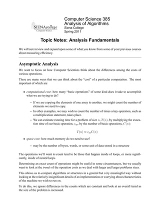
Example 1: Finding the Maximum Element
Our first algorithm to analyze.
max_element(A[0..n-1])
maxval = A[0]
for (i=1 to n-1)
if (A[i] > maxval) maxval = A[i]
return maxval;
The input size parameter is n, the number of elements in the array.
The basic operation could be the comparison or the assignment in the for loop. We choose the
comparison since it executes on every loop iteration.
Since this basic operation executes every time through the loop regardless of the input, the best,
average, and worst cases will all be the same.
We will denote the number of comparisons as C(n). There is one comparison in each iteration of
the loop, so we can (overly formally) specify the total as:
n−1
C(n) = 1 = n − 1 ∈ Θ(n).
i=1
Example 2: Element Uniqueness Problem
Our next example algorithm is one that determines whether all of the elements in a given array are
distinct.
unique_elements(A[0..n-1])
for (i=0 to n-2)
for (j=i+1 to n-1)
if (A[i] == A[j]) return false
return true
8
9. CS 385 Analysis of Algorithms Spring 2011
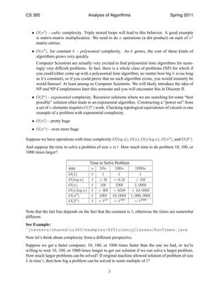
Again, the input size parameter n is the number of elements in the array.
The basic operation is the comparison in the body of the inner loop.
The number of times this comparison executes depends on whether and how quickly a matching
pair is located. The best case is that A[0] and A[1] are equal, resulting in a single comparison.
The average case depends on the expected inputs and how likely matches are. We do not have
enough information to analyze this formally. So we will focus on the worst case, which occurs
when there is no match and all loops execute the maximum number of times.
How many times will the comparison occur in this case? The outer loop executes n − 1 times. For
the first execution of the inner loop, the comparison executes n − 2 times. The second time around,
we do n − 3 comparisons. And so on until the last iteration that executes just once.
So we compute our worst case number of comparisons:
n−2 n−1
C(n) = 1
i=0 j=i+1
n−2
= [(n − 1) − (i + 1) + 1]
i=0
n−2
= (n − 1 − i)
i=0
n−2 n−2
= (n − 1) − i
i=0 i=0
From here, we can factor out the (n − 1) from the first summation and apply the second summation
rule from p. 470 to the second summation to obtain:
n−2
(n − 2)(n − 1)
C(n) = (n − 1) 1−
i=0
2
(n − 2)(n − 1) 2(n − 1)2 (n − 2)(n − 1)
= (n − 1)2 − = −
2 2 2
n(n − 1)
= ∈ Θ(n2 ).
2
This isn’t surprising at all, if we think about what the loops are doing.
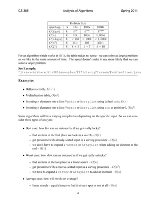
Example 3: Matrix Multiplication
Recall the algorithm for multiplying two n × n matrices:
matmult(A[0..n-1][0..n-1],B[0..n-1][0..n-1])
9
10. CS 385 Analysis of Algorithms Spring 2011
for (i=0 to n-1)
for (j=0 to n-1)
C[i][j] = 0
for (k=0 to n-1)
C[i][j] += A[i][k]*B[k][j]
return C
The input size is measured by n, the order of the matrix.
The basic operation could be the multiplication or the addition in the innermost loop. Generally, we
would choose the multiplication, but since they both happen the same number of times, it doesn’t
matter which we pick We just want to count the number of times that line executes.
The best, average, and worst case behavior are identical: the loops all need to execute to comple-
tion.
So we’re ready to set up our summation for the number of multiplications:
n−1 n−1 n−1 n−1 n−1 n−1
M (n) = 1= n= n2 = n3 .
i=0 j=0 k=0 i=0 j=0 i=0
We can go a step further and estimate a running time, if the cost of a multiplication on a given
machine is cm .
T (n) ≈ cm M (n) = cm n3 .
And this can be extended to include additions (where each of A(n) additions costs ca .
T (n) ≈ cm M (n) + ca A(n) = cm n3 + ca n3 = (cm + ca )n3 .
Which is just a constant multiple of n3 .
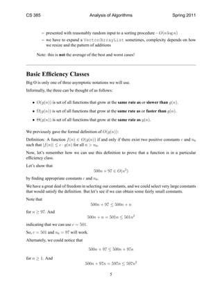
Example 4: Number of Binary Digits Needed for a Number
We next consider a very different example, an algorithm to determine how many bits are needed to
represent a positive integer in binary.
binary(n)
count = 1
while (n > 1)
count++
10
11. CS 385 Analysis of Algorithms Spring 2011
n = floor(n/2)
return count
Our summation techniques will not work here – while this is not a recursive algorithm, the approach
here will involve recurrence relations, which are usually applied to recursive algorithm analysis.
Analyzing Recursive Algorithms
Our approach to the analysis of recursive algorithms differs somewhat. The first three steps are the
same: determining the input size parameter, identifying the basic operation, and separating best,
average, and worst case behavior.
Setting up a summation is replaced by setting up and solving a recurrence relation.
Example 1: Computing a Factorial
A simple recursive solution to find n!:
factorial(n)
if (n==0) return 1
else return n*factorial(n-1)
The size is n and the basic operation is the multiplication in the else part. There is no difference
between best, average, and worst case.
You are very familiar with recurrence relations from Discrete. The recurrence for this problem is
quite simple:
M (n) = M (n − 1) + 1
The total number of multiplications for n! is the number of multiplications for (n − 1)!, plus the 1
to get from n − 1 to n.
We do need a stopping condition for this recurrence, just as we have a stopping condition for the
algorithm. For n = 0, we do not need to do any multiplications, so we can add the initial condition
M (0) = 0.
We can easily determine that M (n) = n just by thinking about this for a few minutes. But instead,
we will worth through this by using back substitution.
M (n) = M (n − 1) + 1
= [M (n − 2) + 1] + 1 = M (n − 2) + 2
= [M (n − 3) + 1] + 1 = M (n − 3) + 3
11
12. CS 385 Analysis of Algorithms Spring 2011
If we continue this pattern, we can get down to
M (n) = M (n − n) + n = M (0) + n = n.
Example 2: Towers of Hanoi
You are all likely to be familiar with the Towers of Hanoi.
Recall that solving an instance of this problem for n disks involves solving an instance of the
problem of size n − 1, moving a single disk, then again solving an instance of the problem of size
n − 1. This leads to the recurrence:
M (n) = 2M (n − 1) + 1
M (1) = 1
Again, we can proceed by backward substitution.
M (n) = 2M (n − 1) + 1
= 2[2M (n − 2) + 1] + 1 = 22 M (n − 2) + 2 + 1
= 22 [2M (n − 3) + 1] + 2 + 1 = 23 M (n − 3) + 22 + 21 + 20 .
Continue this procedure until we obtain
M (n) = 2n−1 M (1) + 2n−2 + 2n−3 + ... + 2 + 1
= 2n−1 + (2n−1 − 1) = 2n − 1 ∈ Θ(2n ).
Example 3: Number of Binary Digits Needed for a Number
We return now to the problem of determining how many bits are needed to represent a positive
integer in binary.
We can recast the problem recursively:
binary_rec(n)
if (n == 1) return 1
else return binary_rec(floor(n/2)) + 1
12
13. CS 385 Analysis of Algorithms Spring 2011
In this case, we will count the number of additions, A(n). For a call to this function, we can see
that A(1) = 0, and
A(n) = A(⌊n/2⌋) + 1
when n > 1.
The problem is a bit complicated by the presence of the floor function. We can only be precise and
apply backward substitution only if we assume that n is a power of 2. Fortunately, we can do this
and still get the correct order of growth (by the smoothness rule).
So assuming n = 2k , we know that A(1) = A(20 ) = 0 and
A(2k ) = A(2k−1 ) + 1
for k > 0. So we can proceed by backward substitution.
A(2k ) = A(2k−1 ) + 1
= [A(2k−2 ) + 1] + 1 = A(2k−2 ) + 2
= [A(2k−3 ) + 1] + 2 = A(2k−3 ) + 3
...
= A(2k−k ) + k = A(20 ) + k = k.
Since n = 2k , k = log2 n, so we have
A(n) = log2 n ∈ Θ(log n).
Empirical Analysis
Much of our work this semester will be a mathematical analysis of the algorithms we study. How-
ever, it is also often useful to perform an empirical analysis – counting operations in or timing an
actual execution of an algorithm.
Let’s see how we can perform a simple empirical analysis one of the algorithms we’ve considered:
matrix-matrix multiplication.
See Example:
˜jteresco/shared/cs385/examples/MatMult
Many factors make such an analysis difficult to perform with any degree of accuracy.
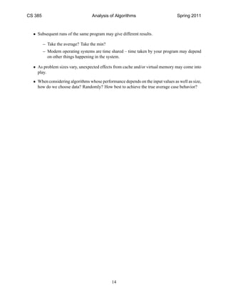
• System clock precision may be quite low. Some very fast operations may measure as 0.
13
14. CS 385 Analysis of Algorithms Spring 2011
• Subsequent runs of the same program may give different results.
– Take the average? Take the min?
– Modern operating systems are time shared – time taken by your program may depend
on other things happening in the system.
• As problem sizes vary, unexpected effects from cache and/or virtual memory may come into
play.
• When considering algorithms whose performance depends on the input values as well as size,
how do we choose data? Randomly? How best to achieve the true average case behavior?
14