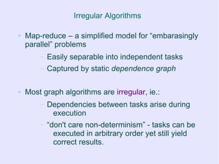
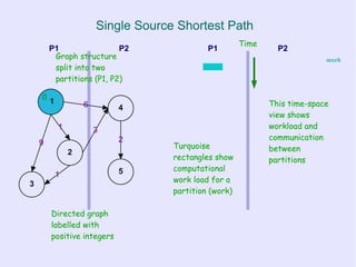
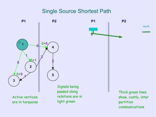
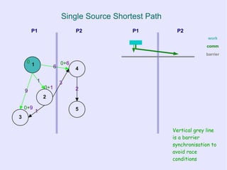
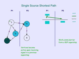
The document discusses processing graph and relational data using MapReduce and Bulk Synchronous Parallel (BSP) models. It describes how most graph algorithms have irregular dependencies between tasks that arise during execution. It provides examples of graph algorithms and discusses challenges in partitioning graph data for parallel processing. It also summarizes the BSP model and how it can be applied to graph algorithms through examples like single-source shortest path.

1. Processing graph/relational data
with
Map-Reduce
and
Bulk Synchronous Parallel
v. 1.1
Tomasz Chodakowski,
1st Bristol Hadoop Workshop, 08-11-2010

2. Irregular Algorithms
● Map-reduce – a simplified model for “embarasingly
parallel” problems
– Easily separable into independent tasks
– Captured by static dependence graph
● Most graph algorithms are irregular, ie.:
– Dependencies between tasks arise during
execution
– “don't care non-determinism” - tasks can be
executed in arbitrary order yet still yield
correct results.

3. Irregular Algorithms
● Often operate on data structures with
complex topologies:
– Graphs, trees, grids, ...
– Where “data elements” are connected by
“relations”
● Computations on such structures depend
strongly on relations between data elements
– primary source of dependencies between
tasks
more in [ADP] “Amorphous Data-parallelism in Irregular Algorithms”

4. Relational Data
● Example relations between elements:
– social interactions (co-authorship,
friendship)
– web links, document references
– linked data or semantic network relations
– geo-spatial relations
– ...
● Different from a relational model
– in that relations are arbitrary

5. Graph Algorithms Rough Classification
● Aggregation, feature extraction
– Not leveraging latent relations
● Network analysis (matrix-based, single relational)
– Geodesic (radius, diameter etc.)
– Spectral (eigenvector-based, centrality)
● Algorithmic/node-based algorithms
– Recommender systems, belief/label
propagation
– Traversal, path detection, interaction
networks, etc.

6. Iterative Vertex-based Graph Algorithms
● Iteratively:
– Compute local function of a vertex that
depends on the vertex state and local
graph structure (neighbourhood)
– and/or Modify local state
– and/or Modify local topology
– pass messages to neighbouring nodes
● -> “vertex-based computation”
Amorphous Data-Parallelism [ADP] operator formulation:
“repeated application of neighbourhood operators in a specific order”

7. Recent applications/developments
● Google work on graph-based YouTube
recommendations:
– Leveraging latent information
– Diffusing interest in sparsely labeled video
clips
● User profiling, sentiment analysis
– Facebook likes, Hunch, Gravity, MusicMetric
...

8. Single Source Shortest Path
Time
P1 P2 P1 P2
Graph structure work
split into two
partitions (P1, P2)
0
1 6 This time-space
4
view shows
1 3 workload and
2 communication
9 Turquoise
2 between
rectangles show partitions
5 computational
1
work load for a
3
partition (work)
Directed graph
labelled with
positive integers

9. Single Source Shortest Path
P1 P2 P1 P2
work
comm
0 0+6
0+6
1 6 4
1 3
0+1
0+1 2
9
2
0+9
0+9 5
1
3
Signals being
passed along Thick green lines
Active vertices relations are in show, costly, inter
are in turquoise light green partition
communications

10. Single Source Shortest Path
P1 P2 P1 P2
work
comm
barrier
0 0+6
0+6
1 6 4
1 3
0+1
0+1 2
9
2
0+9
0+9 5
1
3
Vertical grey line
is a barrier
synchronisation to
avoid race
conditions

11. Single Source Shortest Path
P1 P2 P1 P2
work
comm
barrier
0 work
1 6 6
4
1 3
9 2
1
2
1 5
9
3 Work,comm,barrier
form a BSP superstep
Vertices become
active upon receiving
signal in a previous
superstep

12. Single Source Shortest Path
P1 P2 P1 P2
work
comm
barrier
0 work
1 6 6
4 comm
1+3
1+3
1 3
9 2
1
2
6+2
6+2
1 5
9
3 1+1
1+1
After performing
local computation
they send signals to
their neighbouring
vertices

13. Single Source Shortest Path
P1 P2 P1 P2
work
comm
barrier
0 work
1 6 6
4 comm
1+3
1+3 barrier
1 3
9 2
1
2
6+2
6+2
1 5
9
3 1+1
1+1

14. Single Source Shortest Path
P1 P2 P1 P2
work
comm
barrier
0 work
1 6 4
4 comm
barrier
1 3
work
9 2
1
2
8
1 5
9
3

15. Single Source Shortest Path
P1 P2 P1 P2
work
comm
barrier
0 work
1 6 4
4 comm
barrier
1 3
work
9 2
1 comm
2
4+2
4+2
8
1 5
9
3

16. Single Source Shortest Path
P1 P2 P1 P2
work
comm
barrier
0 work
1 6 4
4 comm
barrier
1 3
work
9 2
1 comm
2
4+2
4+2
barrier
8
1 5
9
3

17. Single Source Shortest Path
P1 P2 P1 P2
work
comm
barrier
0 work
1 6 4
4 comm
barrier
1 3
work
9 2
1 comm
2
barrier
6
1 5
9 work
3

18. Single Source Shortest Path
P1 P2 P1 P2
work
comm
barrier
0 work
1 6 4
4 comm
barrier
1 3
work
9 2
1 comm
2
barrier
6
1 5
9 work
comm
3 barrier
Computation ends when
there are no active
vertices left

19. Bulk Synchronous Parallel
superstep P1 P2 ... Pn
0 w0
h0
l0
1 w1
h1
l1
2 w2
h2
l2
3
w3
h3
... l3
... ... ... ...
Time to finish work on slowest partition +
superstep n cost =
cost of bulk communication +
wn + hn + ln barrier synchronization time

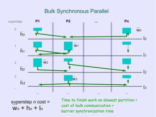
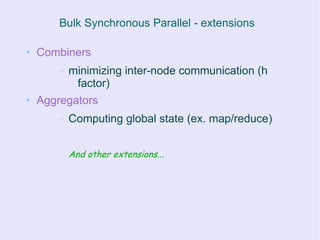
20. Bulk Synchronous Parallel
● Advantages
– Simple and portable execution model
– Clear cost model
– No concurrency control, no data races,
deadlocks, etc.
● Disadvantages
– Coarse grained
●Depends on a large “parallel slack”
– Requires well-partitioned problem space for
efficiency (well balanced partitions)
more in [BSP] “A bridging model for parallel computation”

21. Bulk Synchronous Parallel - extensions
● Combiners
– minimizing inter-node communication (h
factor)
● Aggregators
– Computing global state (ex. map/reduce)
And other extensions...

22. public void superStep() {
Sample code
int minDist = this.isStartingElement() ? 0 : Integer.MAX_VALUE;
for(DistanceMessage msg: messages()) { // Choose min. proposed distance
for(DistanceMessage
minDist = Math.min( minDist, msg.getDistance() );
}
if( minDist < this.getCurrentDistance() ) { //If improves the path, store and propagate
if(
this.setCurrentDistance(minDist);
IVertex v = this.getElement();
for(IEdge r: v.getOutgoingEdges(DemoRelationshipTypes.KNOWS) ) {
for(IEdge
IElement recipient = r.getOtherElement(v);
int rDist = this.getLengthOf(r);
this.sendMessage( new DistanceMessage(minDist+rDist, recipient.getId()) );
}}

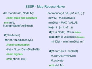
23. SSSP - Map-Reduce Naive
● Idea [DPMR]:
– In map phase:
● emit both signals and local vertex
structure and state
– In reduce phase:
● gather signals and local vertex
structure messages
● reconstruct vertex structure and state

24. SSSP - Map-Reduce Naive
def map(Id nId, Node N): def reduce(Id rId, {m1,m2,..} ):
//emit state and structure new M; M.deActivate
emit(nId, minDist = MAX_VALUE
N.graphStateAndStruct)
for(m in {m1,m2,..})
if(m is Node) M:=m //state
if(N.isActive)
else if(m is Distance) //signals
for(nbr :N.adjacencyL)
minDist = min( minDist, m )
//local computation
dist:= N.currDist+DistToNbr
if(M.currDist > minDist)
//emit signals
M.currDist:=minDist;
emit(nbr.id, dist)
M.activate
emit(rId, M)

25. SSSP - Map Reduce Naive - issues
● Cost associated with marshaling intermediate
<k,v> pairs for combiners (which are optional)
– -> in-line combiner
● Need to pass the whole graph state and structure
around
– -> “Shimmy trick” -- pin down the structure
● Partitions verticies without regard to graph
topology
– -> cluster highly connected components
together

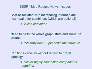
26. Inline Combiners
● In job configure:
– Initialize a map<NodeId, Distance>;
● In job map operation:
– Do not emit interm. pairs ( emit(nbr.id, dist) ) ;
– Store them in the local map;
– Combine values in the same slots.
● In job close:
– Emit a value from each slot in the map to a
corresponding neighbour
● emit(nbr.id, map[nbr.id])

27. “Shimmy trick”
● Store graph structure in a file system (no shuffle)
● Inspired by a parallel merge join
partition p1 p1
p2 p2
p3 p3
sorted by join key sorted and partitioned by join key

28. “Shimmy trick”
● Assume:
– Graph G representation sorted by node ids;
– G partitioned into n parts: G1, G2, .., Gn
– Use the same partitioner as in MR
– Set number of reducers to n
● The above gives us:
– Reducer Ri, receives the same intermediate
keys as those in Gi graph partition (in
sorted order).

29. “Shimmy trick”
def configure( ): def reduce(Id rId, {m1,m2,..} ):
P.openGraphPartition() repeat:
(id nId, node N) <- P.read()
if (nId != rId): N.deact; emit(nId, N)
until: nId == rId
minDist = MAX_VALUE
for(m in {m1,m2,..}):
def close( ): minDist = min( minDist, m )
repeat: if(N.currDist > minDist)
(id nId, node N) <-P.read() N.currDist:=minDist;
N.deactivate N.activate
emit(nId, N) emit(rId, N)

30. “Shimmy trick”
● Improvements:
– Files containing graph structure reside on
dfs
– Reducers arbitrarily assigned to cluster
machines
● -> remote reads.
● -> change the scheduler to assign key ranges to
the same machines consistently.

31. Topology-aware Partitioner
● Choose a partitioner that:
– minimizes inter-block traffic;
– maximizes intra-block traffic;
– places adjacent nodes in the same block
● Difficult to achieve particularly with many real world
datasets:
– Power-law distributions
– Reported that state of the art partitioners
(ex. parmetis) fail for such cases (???)

32. MR Graph Processing Design Pattern
● [DPMR] reports 60% 70% improvement over naive
implementation
● Solution closely resembles the BSP model

33. BSP (inspired) implementations
● Google Pregel:
– classic BSP, C++, production
● CMU GraphLab
– inspired by BSP, java, multi-core
– consistency models, custom schedulers
● Apache Hama
– scientific computation package that runs on top of
Hadoop, BSP, MS Dryad (?)
● Signal/Collect (Zurich University)
– Scala, not yet distributed
● ...

34. Open questions
● What problems are particularly suitable for MR and
which ones for BSP – where are the boundaries?
– Topology-based centrality algorithms
(PageRank):
● Algebraic, matrix-based methods vs.
vertex-based ones?
● When considering graph algorithms:
– MR user base vs. BSP ergonomy?
– Performance overheads?
● Relaxing the BSP synchronous schedule -->
“Amorphous data parallelism”

35. POC, Sample Code
● Project Masuria (early stages, 2011-02)
– http://masuria-project.org/
– As much POC of BSP framework as it is
(distributed) OSGI playground.
● Sample code:
– https://github.com/tch/Cloud9 *
– git@git.assembla.com:tch_sandbox.git
– RunSSSPNaive.java
– RunSSSPShimmy.java *
* - expect (my) bugs
Based on Jimmy Lin and Michael Schatz Cloud9 library

36. References
● [ADP] “Amorphous Data-parallelism in Irregular Algorithms”, Keshav
Pingali et al.
● [BSP] “A bridging model for parallel computation”, Leslie G. Valiant
● [DPMR] “Design Patterns for Efficient Graph Algorithms in
MapReduce”, Jimmy Lin and Michael Schatz