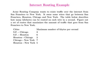
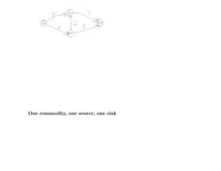
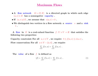
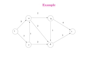
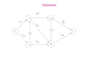
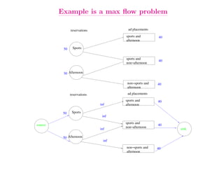
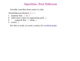
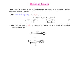
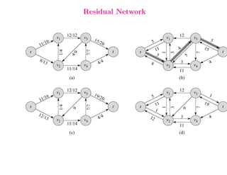
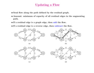
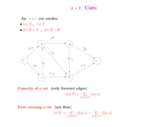
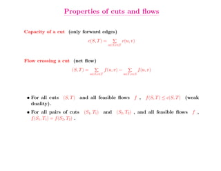
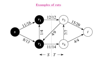
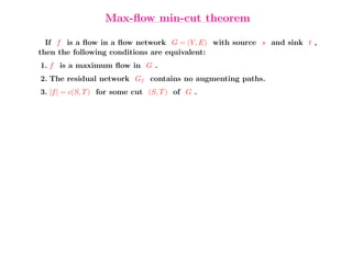
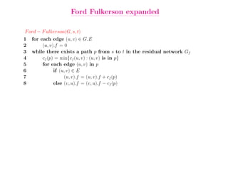
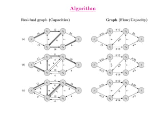
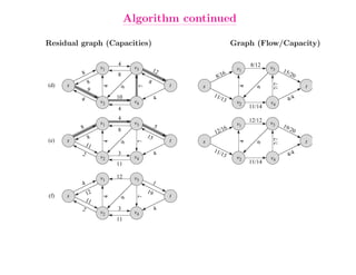
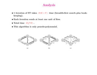
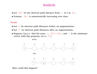
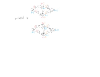
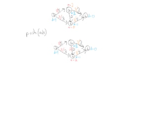
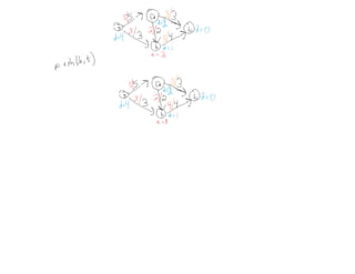
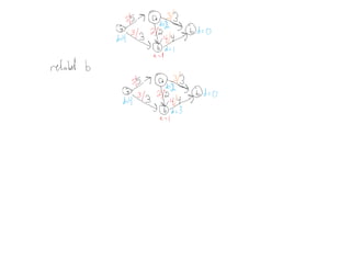
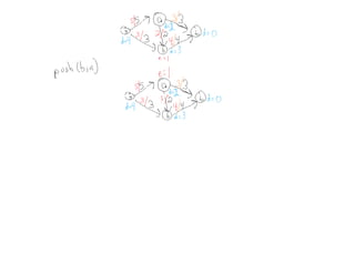
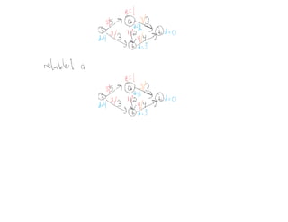
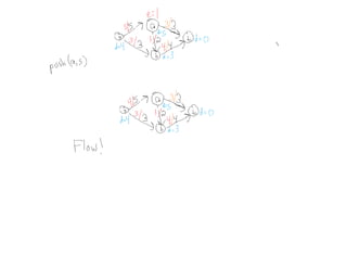
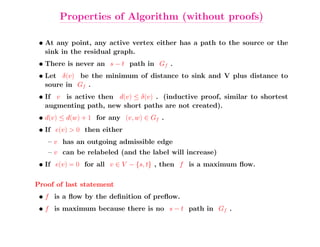
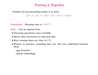
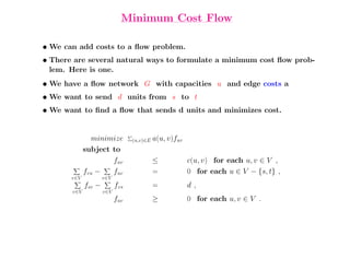
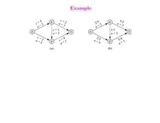
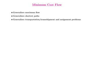
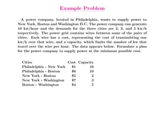
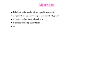
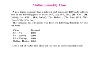
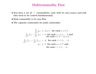
This document summarizes key concepts related to network flows, including maximum flows, minimum cost flows, and multicommodity flows. It provides an example of modeling internet routing as a maximum flow problem. It then describes the Ford-Fulkerson algorithm for finding maximum flows and some of its properties, including that the maximum flow equals the minimum cut. It discusses how the algorithm works by finding augmenting paths in the residual graph and updating the flow. Finally, it analyzes the running time of Ford-Fulkerson and describes how using shortest augmenting paths leads to a polynomial time algorithm.

1. Cliff Stein
Department of Industrial Engineering and Operations
Research
Department of Computer Science
School of Engineering and Applied Science
Columbia University

2. Part 1: Network Flows
• Maximum Flows (in detail)
• Minimum Cost Flows
• Multicommodity Flows

3. Internet Routing Example
Acme Routing Company wants to route traffic over the internet from
San Fransisco to New York. It owns some wires that go between San
Francisco, Houston, Chicago and New York. The table below describes
how many kilobytes can be routed on each wire in a second. Figure out
a set of routes that maximizes the amount of traffic that goes from San
Francisco to New York.
Cities Maximum number of kbytes per second
S.F. - Chicago 3
S.F. - Houston 6
Houston - Chicago 2
Chicago - New York 7
Houston - New York 5

4. One commodity, one source, one sink

5. Maximum Flows
• A flow network G = (V, E) is a directed graph in which each edge
(u, v) ∈ E has a nonnegative capacity .
• If (u, v) ∈ E , we assume that c(u, v) = 0 .
• We distinguish two vertices in a flow network: a source s and a sink
t.
A flow in G is a real-valued function f : V × V → R that satisfies the
following two properties:
Capacity constraint: For all u, v ∈ V , we require 0 ≤ f (u, v) ≤ c(u, v) .
Flow conservation: For all u ∈ V − {s, t} , we require
f (v, u) = f (u, v) .
v∈V v∈V
The value of a flow f is defined as
|f | = f (s, v) − f (v, s) , (1)
v∈V v∈V

6. Example
2
a b
5
4
2
s 1
t
1
3 3
2
c d

7. Solutions
2/ 2
a b
2/ 5 2/
4
1/
2
0/ 1
s t
1/ 1
3/ 3 3/ 3
2/ 2
c d

8. Internet Advertising

10. Availability Queries
Given:
• Forecasts on ad impressions for each publisher’s slot
• A reservation request
Compute: The maximum number of reservations that can be satisfied
from the reservation request.

11. Example
An advertiser wants:
• 50 placements on sports slots
• 50 placements on afternoon slots
Publisher is offering
• 40 placements on slots that are sports and non-afternoon
• 40 placements on slots that are sports and afternoon
• 40 placements on slots that are non-sports and afternoon
reservations ad placements
sports and 40
afternoon
50 Sports
sports and
40
non−afternoon
50 Afternoon
non−sports and 40
afternoon

12. Example is a max flow problem
reservations ad placements
sports and 40
afternoon
50 Sports
sports and
40
non−afternoon
50 Afternoon
non−sports and 40
afternoon
reservations ad placements
sports and 40
inf afternoon
50 Sports
inf
sports and
source 40
non−afternoon
inf sink
50 Afternoon
inf
non−sports and 40
afternoon

13. Algorithm: Ford Fulkerson
Greedily send flow from source to sink.
Ford-Fulkerson-Method (G, s, t)
1 initialize flow f to 0
2 while there exists an augmenting path p
3 augment flow f along p
4 return f
For this to work, we need a notion of a residual graph

14. Residual Graph
The residual graph is the graph of edges on which it is possible to push
flow from source to sink.
• The residual capacity of (u, v) , is







c(u, v) − f (u, v) if (u, v) ∈ E ,
cf (u, v) =  f (v, u)

if (v, u) ∈ E , (2)
 0 otherwise .



• The residual graph Gf is the graph consisting of edges with positive
residual capacity

15. Residual Network
v1 12/12 v3 v1 12 v3
15/ 5
16 20 5
11/
11 15
4
1/4
7/7
s t s t
7
1
3
9
5
4/
5
8/1
3
v2 v4 4/4 8 v2
3
v4
4
11/14 11
(a) (b)
v1 12/12 v3 v1 12 v3
6 19/ 5 1
1 20
11/
11 19
1/4
7/7
s t s t
7
1
3
1
9
9
12/
13
v2 v4 4/4 12
v2
3
v4
4
11/14 11
(c) (d)

16. Updating a Flow
• Send flow along the path defined by the residual graph.
• Amount: minimum of capacity of all residual edges in the augmenting
path.
• If a residual edge is a graph edge, then add the flow.
• If a residual edge is a reverse edge, then subtract the flow.
v1 12/12 v3 v1 12 v3
15/ 5
16 20 5
11/
11 15
4
1/4
s 7/7 t s t
7
1
3
9
5
4/
5
8/1
3
v2 v4 4/4 8 v2
3
v4
4
11/14 11
(a) (b)
v1 12/12 v3 v1 12 v3
19/ 1
16 20 5
11/
11 19
1/4
7/7
s t s t
7
1
3
1
9
9
12/
13
v2 v4 4/4 12
v2
3
v4
4
11/14 11
(c) (d)

17. s - t Cuts
An s - t cut satsfies
•s∈S , t∈T
• S∪T =V , S∩T =∅
2/ 2
a b
2/ 5 2/
4
1/
2
0/ 1
s t
1/ 1
3/ 3 3/ 3
2/ 2
c d
Capacity of a cut (only forward edges)
c(S, T ) = c(u, v)
u∈S,v∈T
Flow crossing a cut (net flow)
(S, T ) = f (u, v) − f (u, v)
u∈S,v∈T u∈T,v∈S

18. Properties of cuts and flows
Capacity of a cut (only forward edges)
c(S, T ) = c(u, v)
u∈S,v∈T
Flow crossing a cut (net flow)
(S, T ) = f (u, v) − f (u, v)
u∈S,v∈T u∈T,v∈S
• For all cuts (S, T ) and all feasible flows f , f (S, T ) ≤ c(S, T ) (weak
duality).
• For all pairs of cuts (S1, T1) and (S2, T2) , and all feasible flows f ,
f (S1, T1) = f (S2, T2) .

19. Examples of cuts
v1 12/12 v3 15/
11/16 20
1/4
7/7
s t
9
4/
8/1
3
v2 v4 4/4
11/14
S T

20. Max-flow min-cut theorem
If f is a flow in a flow network G = (V, E) with source s and sink t ,
then the following conditions are equivalent:
1. f is a maximum flow in G .
2. The residual network Gf contains no augmenting paths.
3. |f | = c(S, T ) for some cut (S, T ) of G .

21. Proof

22. Ford Fulkerson expanded
F ord − F ulkerson(G, s, t)
1 for each edge (u, v) ∈ G.E
2 (u, v).f = 0
3 while there exists a path p from s to t in the residual network Gf
4 cf (p) = min{cf (u, v) : (u, v) is in p}
5 for each edge (u, v) in p
6 if (u, v) ∈ E
7 (u, v).f = (u, v).f + cf (p)
8 else (v, u).f = (v, u).f − cf (p)

23. Algorithm
Residual graph (Capacities) Graph (Flow/Capacity)
v1 12 v3 v1 4/12 v3
16 20 6 20
4/1
(a) s t s t
4
7
4
7
9
4/
9
13 13
v2 v4 4 v2 v4 4/4
14 4/14
8 8/12
v1 v3 v1 v3
12 20 4/2
4 4/16 0
4
4
4/4
(b) s t s t
7
4
7
9
4/
5
13 10 4/1
v2 v4
4 3
v2 v4 4/4
4 4/14
4 8/12
v1 v3 16 v1 v3
12 6 8/2
8 8/1 0
4 4
4
(c) s t s t
4
7
4
7
9
9
5
4/1
4
v2
10
v4
4 3
v2 v4 4/4
4 4/14

24. Algorithm continued
Residual graph (Capacities) Graph (Flow/Capacity)
4 8/12
v1 v3 12 v1 v3
8 15/
8 6 20
8/1
8 8
7/7
(d) s t s t
4
4
7
9
9
9
10 11/
4
v2 v4
4 13
v2 4/4
v4
4 11/14
4 12/12
v1 v3 v1 v3 19/
8 5 6
8 2/1 20
1
8 15
7/7
(e) s t s t
4
4
7
11
9
9
11/
2
v2
3
v4
4 13
v2 4/4
v4
11 11/14
v1 12 v3
4 1
12 19
(f) s t
4
7
11
9
2 3 4
v2 v4
11

25. Analysis
• 1 iteration of FF takes O(E + V ) time (breadth-first search plus book-
keeping).
• Each iteration sends at least one unit of flow.
• Total time O(f ∗E) .
• This algorithm is only psuedo-polynomial.
00 u 1,0 9 u 1,0 99 u 999
,0 00, ,99 00, ,9 ,9
1,000 000 999 000 999 99
1 1 1
s t s t s 999 t
1
1
1
9 99
,99 ,99 ,9
1,0
00, 00
1,0
00, 999 9 999
000 ,0 000 1
v 1,000 v 1 v 1
(a) (b) (c)

26. A polynomial algorithm– Shortest Augmenting Path
Algorithm due to Edmonds and Karp, Dinic
Algorithm
• Run Ford-Fulkerson, but always choose the shortest augmenting path
in the residual graph.
• Breadth-first search implements this algorithm.

27. Idea for Analysis
Intuition
• Augment along shortest path in residual graph.
• Short paths get “saturated” and disappear.
• Future augmenting paths are along longer paths
• Eventually algorithm terminates because no more paths exist (remem-
ber that no augmenting path can have length greater than V.
This doesn’t quite work, but is close

28. Analysis
• Let δ(v) be the shortest path distance from v to t in Gf .
• Lemma: δ(v) is monotonically increasing over time.
Proof:
• Let δ be shortest path distances before an augmentation.
• Let δ be shortest path distances after an augmentation.
• Suppose, f.p.o.c. that for some v , δ (v) > δ(v) , and v is the minimum
vertex with this property (w.r.t δ )
Before
5 4 3 2 1 0
v t
After
4 3 2 1 0
v w t
How could this happen?

29. How could this happen?
Before
5 4 3 2 1 0
v t
After
4 3 2 1 0
v w t
• (v, w) ∈ Gf but not in Gf . (why?)
• We must have sent flow on (w, v) in the augmenting path
• δ(w) = 6
• δ (w) < δ(w) , which contradicts v being the minimum vertex whose
label decreased.
Conclusion: δ(v) never decreases.

30. Analysis Continued
• Each δ(v) increases at most V times.
• Total number of times any δ(v) increases is at most V 2 .
• We need to tie this to an augmenting path.
• Problem: A particular augmenting path may not increase any δ(v) .
(How can this happen?)
Solution We need to find some other event that happens on every aug-
menting path and then relate this event to increasing distances.
Conclusion: δ(v) never decreases.

31. Analysis Continued
• 0 ≤ δ(v) ≤ V
• δ(v) never decreases.
• Each δ(v) increases at most V times.
• Total number of times some δ(v) increases is at most V 2 .
• We need to tie this to an augmenting path.
• Problem: A particular augmenting path may not increase any δ(v) .
(How can this happen?)
Solution We need to find some other event that happens on every aug-
menting path and then relate this event to increasing distances.
Edge Saturation
• If an augmeting path send cf (v, w) units of flow on edge (v, w) then
we call the push saturating.
• Every augmenting path saturates at least one edge. (Why?)

32. Analysis Continued
Edge Saturation
• If an augmeting path send cf (v, w) units of flow on edge (v, w) then
we call the push saturating.
• Every augmenting path saturates at least one edge.
Focus on a particular pair of vertices (v, w)
• Suppose that (v, w) ∈ Gf
• What has to happen between two consecutive saturations of (v, w)

33. Events Between 2 edge saturations
5 4
v w
saturate (v,w)
v w
5 6
v w
saturate (w,v)
v w
7 6
v w
saturate (v,w)
• Both v and w have to be relabeled.
• So each edge can be saturated at most V /2 times.

34. Putting it together
• Each edge (or its reverse) can be saturated at most V /2 times.
• There are most EV edge saturations.
• Each augmenting causes at least one edge saturation
• Therefore, there are at most EV augmenting paths.
• Recall O(E) time per augmenting path.
A max flow can be found in O(E 2V ) time .
Faster augmenting path based algorithms exist, most based on finding
the augmenting paths more efficiently.
• O(V E log V ) (Sleator and Tarjan)
• O(min E 3/2, V 2/3E log(V 2/E) log C) (Goldberg and Rao)

35. Push relabel algorithms
Algorithm due to Goldberg and Tarjan
Ideas
• Maintain variables d(v) which are “distances”, estimates (lower bounds)
on the distance to the sink (or source) in the residual graph
• Push flow over one edge at a time, pushing from a higher distance vertex
to a lower distance vertex.
• Allow excess flow to accumulate at a vertex.
• Maintain a preflow rather than a flow.
Capacity constraint: For all u, v ∈ V , we require 0 ≤ f (u, v) ≤ c(u, v) .
Relaxed Flow conservation: For all u ∈ V − {s, t} , we require
f (v, u) ≥ f (u, v) .
v∈V v∈V
Define excess
e(u) = f (v, u) − f (u, v) (3)
v∈V v∈V

36. Example

38. Comparison with augmenting paths
• Augmenting paths
– Always maintains a flow (feasibility)
– Works towards optimality (maximum flow)
• Push/relabel
– Always maintains a preflow and works towards a flow
– Maintains a superoptimal preflow and moves towards feasibility.

39. Basic Operations
• If e(v) > 0 then v is active.
• If cf (v, w) > 0 and d(v) = d(w) + 1 then (v, w) is admissible.
Push from active vertices over admissible edges.
P ush(u, v)
1 / Applies when: u is active, cf (u, v) > 0, and u.d = v.d + 1.
/
2 / Action: Push f (u, v) = min(u.e, cf (u, v)) units of flow from u to v.
/
3 f (u, v) = min(u.e, cf (u, v))
4 if (u, v) ∈ E
5 (u, v).f = (u, v).f + f (u, v)
6 else (v, u).f = (v, u).f − f (u, v)
7 u.e = u.e − f (u, v)
8 v.e = v.e + f (u, v)
Relabel When a vertex has all its outgoing residual edges pointing uphill,
we relabel it.
Relabel(u)
1 / Applies when: u is active and for all v ∈ V such that (u, v) ∈ Ef ,
/
we have u.d ≤ v.d .
2 / Action: Increase the label of u.
/
3 u.d = 1 + min{v.d : (u, v) ∈ Ef }

40. Generic Push Relabel Algorithm
Initialize − P ref low(G, s)
1 for each vertex v ∈ G.V
2 v.d = 0
3 v.e = 0
4 for each edge (u, v) ∈ G.E
5 (u, v).f = 0
6 s.d = |G.V |
7 for each vertex v ∈ s.Adj
8 (s, v).f = c(s, v)
9 v.e = c(s, v)
10 s.e = s.e − c(s, v)
Generic − P ush − Relabel(G)
1 Initialize-Preflow(G, s)
2 while there exists an applicable push or relabel operation
3 select an applicable push or relabel operation and perform it

41. Run Through Example

51. Properties of Algorithm (without proofs)
• At any point, any active vertex either has a path to the source or the
sink in the residual graph.
• There is never an s − t path in Gf .
• Let δ(v) be the minimum of distance to sink and V plus distance to
soure in Gf .
• If v is active then d(v) ≤ δ(v) . (inductive proof, similar to shortest
augmenting path, new short paths are not created).
• d(v) ≤ d(w) + 1 for any (v, w) ∈ Gf .
• If e(v) > 0 then either
– v has an outgoing admissible edge
– v can be relabeled (and the label will increase)
• If e(v) = 0 for all v ∈ V − {s, t} , then f is a maximum flow.
Proof of last statement
• f is a flow by the definition of preflow.
• f is maximum because there is no s − t path in Gf .

52. Running Time
We will need to bound
1. Number of relabels
2. Time per relabel
3. Number of pushes
4. Time per push
5. Bookkeeping time

53. Easy ones:
Relabel(u)
1 / Applies when: u is active and for all v ∈ V such that (u, v) ∈ Ef ,
/
we have u.d ≤ v.d .
2 / Action: Increase the label of u.
/
3 u.d = 1 + min{v.d : (u, v) ∈ Ef }
Time per relabel
• Easy bound: O(V )
• Time to relabel each vertex once : O(V 2)

54. Easy ones:
Relabel(u)
1 / Applies when: u is active and for all v ∈ V such that (u, v) ∈ Ef ,
/
we have u.d ≤ v.d .
2 / Action: Increase the label of u.
/
3 u.d = 1 + min{v.d : (u, v) ∈ Ef }
Time per relabel
• Easy bound: O(V )
• Time to relabel each vertex once : O(V 2)
• Better bound: O(degree(v))
• Time to relabel each vertex once: v degree(v) = O(E)
(This is an example of amortized analysis)
Number of relabels
• Vertex labels are at most 2V , so each vertex is relabelled at most 2V
times.
• Total time spent relabelling = V v degree(v) = O(EV )

55. Pushes
P ush(u, v)
1 / Applies when: u is active, cf (u, v) > 0, and u.d = v.d + 1.
/
2 / Action: Push f (u, v) = min(u.e, cf (u, v)) units of flow from u to v.
/
3 f (u, v) = min(u.e, cf (u, v))
4 if (u, v) ∈ E
5 (u, v).f = (u, v).f + f (u, v)
6 else (v, u).f = (v, u).f − f (u, v)
7 u.e = u.e − f (u, v)
8 v.e = v.e + f (u, v)
Easy part
• Time per push = O(1) .
• Bookkeeping (can be amortized against other operations with reason-
able data structures and rules for choosing push/relabel operations).
Two types of Pushes
• Saturating push: Sends cf (v, w)) flow on (v, w)
• Non-saturating push: Sends less flow. ( e(v) ).

56. Bounding Saturating Pushes
Consider a saturating push on (v, w) . What has to happen before the
next saturating push on (v, w) ?

57. Bounding Saturating Pushes
Consider a saturating push on (v, w) . What has to happen before the
next saturating push on (v, w) ?
• w has to be relabelled
• A push on (w, v) must occur
• v has to be relabelled.
Conclusion
• Between any two saturating pushes on (v, w) , v must be relabelled.
• v can be relabelled at most 2V times.
• There are at most 2V saturating pushes on (v, w) .
• The total number of saturating pushes is O(V E) .

58. Non-saturating pushes
Issue After a non-saturating push, the graph does not change, nothing
need be relabelled and another non-saturating push can occur on the edge
before anything significant happnes.
Solution As with shortest-augmeting-path, we won’t count directly, but
will bound other operations and related to non-saturating pushes. We will
do so via means of a potential function.
Φ= d(v)
v:e(v)>0

59. Analysis
Φ= d(v)
v:e(v)>0
• After initialiazation Φ ≤ 2V 2.
• At termination Φ = 0 .
• Let R be total increase in Φ due to relabellings.
• Let S be total increase in Φ due to saturating pushes.
• Each non-saturating push decreases Φ by at least 1. (Why?).

61. Putting these facts together
• Total decrease in Φ associated with non-saturating pushes is at most
2V 2 − 0 + R + S .
• Each non-saturating push decreases Φ by at least 1. (Why?).
• Number of non-saturating pushes is at most 2V 2 − 0 + R + S .

62. Bounding R and S
Φ= d(v)
v:e(v)>0
Relabellings
• Each relabelling must increase Φ by at least 1.
• Total increase in Φ associated with relabelling v is at most 2V .
• Total increase associated with all relabellings is at most 2V 2 .
Saturating Pushes
• A saturating push leaves excess at v . It adds excess to w .
– If w already had excess, then Φ is unchanged.
– If w did not have excess, then Φ increases by d(w) , which is at
most 2V .
• There are at most O(EV ) saturating pushes, therefore total increase
due to saturating pushes is O(EV 2) .

63. Putting it Together
Number of non-saturating pushes is at most
2V 2 − 0 + R + S = O(V 2 + EV + EV 2) = O(EV 2)
.
Conclusion: Running time is O(EV 2) .
Note: Can be improved by
• Choosing operations more carefully.
• Better data structures to represent flow
• Best running times are close to V E.
• Winner in practice, assuming that one uses two additional heuristic
ideas
– gap heuristic
– global relabellings

64. Minimum Cost Flow
• We can add costs to a flow problem.
• There are several natural ways to formulate a minimum cost flow prob-
lem. Here is one.
• We have a flow network G with capacities u and edge costs a
• We want to send d units from s to t
• We want to find a flow that sends d units and minimizes cost.
minimize (u,v)∈E a(u, v)fuv
subject to
fuv ≤ c(u, v) for each u, v ∈ V ,
fvu − fuv = 0 for each u ∈ V − {s, t} ,
v∈V v∈V
fsv − fvs = d,
v∈V v∈V
fuv ≥ 0 for each u, v ∈ V .

65. Example
5 c= 1/2
x a= 2 2/5 2 x
c= 2 a=
a= 7 a= 7
c=1 1/1
s t s t
a=3 a=3
c= 4 2/2
a= 2 y c= 1 a= y 3/4 1
5 a= 5 a=
(a) (b)

66. Minimum Cost Flow
• Generalizes maximum flow
• Generalizes shortest paths
• Generalizes transportation/transshipment and assignment problems

67. Example Problem
A power company, located in Philadelphia, wants to supply power to
New York, Boston and Washington D.C. The power company can generate
10 kw/hour and the demands for the three cities are 2, 3, and 5 kw/h
respectively. The power grid contains wires between some of the pairs of
cities. Each wire has a cost, representing the cost of transimitting one
kw/h over that wire, and a capacity, which limits the number of kw that
travel over the wire per hour. The data appears below. Formulate a plan
for the power company to supply power at the minimum possible cost.
Cities Cost Capacity
Philadelphia - New York $1 10
Philadelphia - Boston $6 10
New York - Boston $2 2
New York - Washington $7 3
Boston - Washington $4 5

68. Algorithms
• Efficient polynomial time algorithms exist.
• Augment along shortest path in residual graph
• A push relabel type algorithm
• Capacity scaling algorithms
• ...

69. Multicommodity Flow
A new phone company has a network that can route 2000 calls between
each of the following pairs of cities: (SF, LA), (SF, Bos), (SF, Chi.) (SF,
Dallas), (LA, Chi.) , (LA, Dallas), (Chi. Dallas) , (Chi, Bos), (Chi., NY),
(Dal., NY), (NY, Bos).
The company has customers who have the following demands for calls
per hour:
Cities Demand
SF - NY 1000
SF - Boston 3000
LA - Chicago 4000
Dallas - Boston 2000
Give a set of routes that allow all the calls to occur simultaneously.

70. Multicommodity Flow
• You have a set of k commodities, each with its own source and sink
that need to be routed simultaneously.
• Each commodity is its own flow.
• The capacity constraints are joint constraints.
k
fiuv ≤ c(u, v) for each u, v ∈ V ,
i=1
fiuv − fivu = 0 for each i = 1, 2, . . . , k and
v∈V v∈V for each u ∈ V − {si, ti} ,
fi,si,v − fi,v,si = di for each i = 1, 2, . . . , k ,
v∈V v∈V
fiuv ≥ 0 for each u, v ∈ V and
for each i = 1, 2, . . . , k .

71. Multicommodity Flow Algorithms
• Multicommodity flow, like minimum cost flow and maximum flow is
a linear program (min/max a linear objective subject to linear con-
straints.)
• Polynomial-sized linear programs can be solved in polynomial time.
• Linear programs, in general, do not necessarily return integer solutions.
• Max flow and min-cost flow, given integral data, do have optimal integral
solutions. Standard algorithms find optimal integeral solutions.
• Multicommodity flow does not, in general have optimal integral solu-
tions.
• Finding an optimal (real-valued) solution to a multicommodity flow
problem is much harder (but still polynomial) than a similar sized max-
imum or minimum-cost flow problem. In practice, it’s pretty slow.
• Finding an optimal integral solution to a multicommodity flow problem
is NP-hard.

72. Example